Quantitative Techniques for Competition and Antitrust Analysis_6 docx

4.1. Basic Concepts in Market Definition 163
heavily constrained—it cannot raise the price beyond the point where too many con-
sumers would switch. Intuitively, we will argue that if this constraint is large enough
to impose a significant restriction on the electricity producer’s ability to increase
prices, then the market should be defined as the energy market (electricity plus gas or
coal) and inthis wider market the electricitymonopolist will have little market power.
In the paragraph above we have drawn a clear distinction between a world where
very few consumers would switch following a price rise and a world where many
consumers would switch following a price rise. In practice, of course, the world is
often far less black and white and as a result we may ask how much price sensitivity
is enough to define a narrow market? When does the ability to differentiate turn
into market power? When is substitution “large enough”? How much substitution
exactly does one need between two products to put them in the same market? Nat-
urally, theory provides only very partial answers to such questions and as a result
practitioners commonly use quantitative benchmarks that are generally accepted
and which ensure some consistency in the decision-making process. For example,
in much of the discussion that follows, we will consider whether price increases
of 5% or 10% are profitable when defining markets. Even then it is important to
note that market definition in practice often requires the exercise of evidence-based
judgment, where the evidence can be of varying quality.
4.1.2 Supply and Demand Substitutability
The key factors that limit market power—the ability to raise prices above the com-
petitive level—are the extent of demand substitutability and the extent and nature of
supply reaction, in particular, of supply substitutability. We describe each of these
concepts below since any market definition exercise will examine each of them in
detail. We also describe the fact that a market definition exercise usually proceeds
along two dimensions: (1) a product market definition dimension and (2) a geo-
graphical market definition dimension. Product and geographic market definition
should, in principle, be considered together. However, it is common practice as a
practical matter to examine first product market substitution on the demand and
supply sides and then to go on to consider geographic market substitution, again on

the demand and supply sides. In each case, the market definition process usually
begins with a single candidate product, or occasionally with a collection of them.
Demand substitutability describes the extent to which buyers respond to a price
increase by substituting away to alternative products (product market definition) or
alternative locations (geographic market definition). For example, if the price of
gold goes up, then consumers may switch their consumption by buying less gold
and perhaps more silver. If, when a firm attempts to increase its price, “enough”
of her customers switch to substitute goods, then clearly her ability to raise prices
is severely constrained. We want to include substitute products in our competition
policy market whenever “enough” buyers, in a sense that will be made more precise
164 4. Market Definition
below, would switch in response to a price increase. Of course, goods to which
consumers do not switch in response to a price increase should be excluded from
the market. Geographic market definition on the demand side considers the extent
to which increasing a price in one area would induce consumers to purchase from
alternative localities.
There are numerous difficulties (and therefore fascinations) in such an apparently
simple activity as evaluating demand substitutability. One common difficulty faced
in practice is that sometimes there are simply no real potential close “substitute”
products, or, alternatively, sometimes there are a very large number of them.
3
In the
absence of identifiable discrete potential substitutes, a competition authority may
capture demand substitution away to a diffuse set of alternatives by ignoring the
substitution during the market definition phase of an investigation. In doing so, we
must be sure to take proper account of it later during the competitive assessment
phase of the investigation. This approach can lead to a relatively narrow market
definition, but it does not mean the agency will find competition problems since
even a monopolist can face a highly elastic demand curve and therefore have no
ability to raise prices. Specifically, that will be the case when attempts to do so

would be met by substitution of expenditure to other activities, even if they are only
specified generically as an “outside” alternative.
Supplier substitutability describes suppliers’ responses to an increase in a prod-
uct’s price. When prices increase, consumers respond but so may rival suppliers
since with higher prices available they have greater incentives to produce output.
For example, in the market for liquid egg products
4
(such as those used for producing
omelettes), the equipment used for processing and putting the product into cartons
can also be used to produce cartons of fruit smoothies. That fact means that if the
price of liquid egg went up sufficiently, suppliers of smoothies may potentially sub-
stitute their production capacity to produce processed egg. Another example might
involve red and yellow paint—if it is easy to switch machines from producing red
paint to producing yellow paint, the returns to producing these two products can
never be far apart. If yellow paint producers were more profitable than red paint
producers, then we would soon enough induce some of the red paint producers to
switch to producing yellow paint.
As with all apparently simple concepts, there are numerous questions about ex-
actly what is meant by supply substitutability. For example, the current Commission
3
An example of the latter includes the U.K. CC’s investigation into a “soft” gambling product known
as the “Football Pools.” That inquiry received evidence from a survey of consumers who had recently
stopped playing the Football Pools about their reasons for doing so. The survey found that 65% of lapsed
customers had not switched expenditure to any kind of gambling product, while they had saved the money
for a large variety of alternative uses, most of which were not obviously best considered as potential
substitutes (see www.competition-commission.org.uk/inquiries/ref2007/sportech/index.htm).
4
See, for example, the discussion of the liquid egg market in Stonegate Farmers Ltd/Deans Foods
Group Ltd (www.competition-commission.org.uk/inquiries/ref2006/stonegate/index.htm).
4.1. Basic Concepts in Market Definition 165

Notice on Market Definition
5
does not require a case officer to consider potential
entrants as a source of supply substitutability for market definition purposes, though
such entry might easily be considered in a more general sense a source of supply
substitutability. Rather, the guidelines suggest that it is better to leave the analysis of
the constraints imposed by potential competition to a later phase of the investigation.
The rationale is that, among other things, the effects of entry are unlikely to be
immediate. Still, economic theory says that, in some limited circumstances, even
potential entrants may impose a price constraint on existing market players (see
Baumol et al. 1982; Bailey 1981). This happens, for example, when incumbent’s
prices are hard to adjust and potential entrants interpret current prices as being the
prices for the post-entry situation. In this case, the incumbent needs to maintain a
pre-entry price that is low enough to discourage entry. Thus, important judgements
are often made around supply substitutability both in individual cases and in the
guidance documents from various jurisdictions. To return to our earlier examples,
one response to the red and yellow paint example might be to argue that supply
substitution implies that the appropriate market definition involves one market for
“paint.” Such an argument can be compelling, but there are significant limits to the
appropriate scope of this type of argument for market definition. To see why, let us
turn to the liquidegg and smoothie example. In thatcase, raw supply-side logicmight
suggest a market definition would include both liquid egg and smoothies. However,
such a conclusion appears to bean odd onesince these are patently different products.
In fact, agencies would probably take the view that the appropriate responsewould be
to view the potential movement of packaging and processing equipment as a supply
response within the market for liquid egg. After all, the constraint arises on the liquid
egg producers because machine capacity is moved across to produce liquid eggs
and not because liquid eggs and smoothies are really competing, although the firms
producing them may well be. The draft 2009 U.K. merger guidelines, for example,
follow the U.S. guidelines in using this logic to suggest that demand substitution

should play the primary role in defining the market while supply substitutability may
tell us about the identity and scale of, in particular, potential competitors within that
market. Thus the market would be for liquid egg, but the set of potential competitors
may involve liquid egg and (formerly) smoothie producers.
Finally, we note that the responses by rivals can be to enter or expand production
following a price rise but theory suggests the response may also be to increase
prices since prices are strategic complements. While quantity reactions by rivals
may decrease the profitability of attempted price increases, price reactions by rivals
to price increases may reinforce their profitability. It would appear to be an odd
market definition practice that treated price and quantity responses asymmetrically
irrespective of the context. Thus, practice has evolved to recognize the potential
role of supply substitution but also to recognize that its role is limited for market
5
Commission Notice on Market Definition, OJ C 372 9/12/1997.
166 4. Market Definition
definition. (See also the EU Notice on the Definition of the Relevant Market for the
Purposes of Community Competition Law, which similarly significantly constrains
the role of supply substitutability in market definition.)
4.1.3 Qualitative Assessment
Before we progress to consider quantitative approaches to market definition, it is
worth emphasizing that much of the time market definition relies at least in part on
qualitative assessment. Indeed, qualitative evaluation is universally the starting point
of any market definition exercise. Clearly,for example, it isprobably not necessary to
do any formal market analysis to get to the conclusion that the price of ice cream will
not be sensitive to the price for hammers. Indeed, if such qualitative assessments
were not possible, it would be necessary to do a huge amount of work in every
investigation to check out every possibility—an impossibility at current resource
levels in most authorities. In practice, we can narrow down the set of possibilities to
those which are plausible and also substantive. Very minor products, for example,
may just not make a great difference to a competition evaluation. To do so, it is best

to start with the product characteristics and the intended use(s) of the product. Doing
so allows the investigator to define a broad and yet plausible set of possible demand
substitutes. The products which are substitutes in use are sometimes known as the
set of “functional” substitutes.
For our purposes the concept of market definition is designed primarily to describe
the set of products which constrain a firm’s pricing decisions. Thus, to be included
in a market, it is not enough for products to be functional substitutes; they need to
be good enough demand or (to the extent appropriate) supply substitutes to actu-
ally constrain each other’s price. To illustrate the distinction, consider two differ-
ent seafoods: smoked salmon and caviar. Both will be familiar items at least in
terms of existence, even if the latter is not a regular feature of most of our dinner
tables. Caviar is potentially a functional substitute for smoked salmon in that it
could be served as part of a salad. Would that suffice to put smoked salmon into
a broader market that includes caviar? To answer that question we must first con-
sider the extent of demand substitutability at competitive prices, which for present
purposes we can take as current prices. At the moment, the retail price of 100 g
of smoked salmon in Europe can oscillate around €1.50–2.00. The price of 100 g
of caviar can run into hundreds of euros. Intuitively, since the price of the smoked
salmon is far below the price of caviar, those customers who consider the two
to be close substitutes will be eating smoked salmon in their salads. Similarly,
those who do not really like caviar will be eating smoked salmon while only those
with a particularly intense taste for caviar will be prepared to pay such a large
premium for it.
6
On the other hand, many of the consumers of smoked salmon
6
The reader will, of course, have picked up that we should probably worry about whether the fact that
salmon and caviar need not be consumed in equal quantities is important. To aid discussion we will put
4.1. Basic Concepts in Market Definition 167
may like caviar and consider it to be a perfectly acceptable functional substitute

at least in some uses (e.g., pre-dinner canapes), but would not actually substitute
at current price levels. The lesson is that in a world with only those two products,
salmon would be considered a market in itself at current price levels, despite the
fact that caviar is indeed a functional substitute in many applications for current
customers of salmon. Note that the force in this argument relies on the current price
differential driving the set of current consumers of salmon to include those con-
sumers for whom caviar may be a perfectly good functional substitute but caviar
is so expensive that it is not a demand substitute. Since the extent of demand sub-
stitutability between goods depends on their relative price levels, if prices were
different, then the appropriate competition policy market definition could also be
different.
While such intuitive and unstructured arguments can be helpful, both formal and
informal market definition exercises typically use the hypothetical monopolist test
(HMT; see section 4.5 below for an extensive discussion) as a helpful framework for
structuring decision making. The HMT test suggests that markets should be defined
as the smallest set of products which can profitably be monopolized. The basic
idea is that firms/products outside such a market cannot be significantly constrain-
ing behavior of firms inside the market since they cannot constrain a hypothetical
monopolist of all the products in the market. Usually, the HMT is described in terms
of price, so we ask whether the hypothetical monopolist would be able to exploit a
material degree of market power, that is, to raise the prices of goods inside the can-
didate market by a small but significant amount. Of course, since firms can compete
in quality, service, quantity, or even innovation, in principle the test can be framed
using any of these competitive variables.
Qualitative analysis can sometimes be enough to satisfactorily define the relevant
market, indeed it is sometimes necessary to rely on purely qualitative analysis. That
said, a more explicitly quantitative analysis of market data will often be very helpful
for informing and supplementing our judgments in this area.
4.1.4 Supplementing Qualitative Evidence
We will explore in detail a whole array of quantitative techniques for market defi-

nition in the rest of this chapter. Before we do so, however, it is worth noting that
an important element of the qualitative assessment typically involves an evaluation
of the extent to which consumers view products as functional substitutes. While a
qualitative assessment of (1) the various product characteristics of goods and (2) the
uses to which consumers put the goods is usually helpful and sometimes all that
is available, it is often possible to supplement such qualitative evidence with more
quantitative evidence.
this issue to one side. The key question will remain whether enough consumers will substitute enough
volume from salmon to caviar to make increases in the price of salmon unprofitable.
168 4. Market Definition
Table 4.1. Characteristics of London airports.
Public Airport denomination
Distance transport on Ryanair website;
to center Private
‚
…„ ƒ
bus service to
of city car Bus Rail city promoted on
Airports (km) (min) (min) (min) Ryanair website
Stansted 59 85 75 45 London (Stansted);
Ryanair bus service
Heathrow 28 65 65 55 Not served by Ryanair
Gatwick 46 85 90 60 London (Gatwick)
Luton 54 44 60 25 London (Luton);
Ryanair bus service
London City 14 20 — 22 Not served by Ryanair
Source: Ryanair and Aer Lingus proposed concentration, Case no. COMP/M.4439, p. 33.
To illustrate, consider the evidence provided to the European Commission in its
investigation of the proposed merger between Ryanair and Aer Lingus.
7

Ryanair
argued that the London airports were not demand substitutes, at least for time-
sensitive passengers. Consider table 4.1, which documents the time taken by various
transport modes to each London airport from the center of the city, which brings
some data to bear on the question of whether these airports are “too different” to
be considered functional substitutes for customers who want to go from London to
Dublin. Ryanair argued they were, while the Commission noted, among other things,
that the U.K. Civil Aviation Authority considers that a “two-hour surface access
time” is the relevant benchmark for airport catchment areas for leisure passengers.
The Commission concluded that scheduled point-to-point passenger air transport
services between Dublin and London Heathrow, Gatwick, Stansted, Luton, and
City airports belong to the same market. Note that although the Commission has
quantified an important set of characteristics of the potentially substitute products
in a manner that helps it understand the extent of substitutability, it must ultimately
make a judgment about whether these products are similar enough to be considered
in the same market on the basis of this and other evidence.
Analysis of consumers’ tastes can also help inform the question of substitutability.
Continuing our discussion of the Ryanair andAer Linguscase, consider, forexample,
the survey of passengers at Dublin airport that the Commission undertook. A sample
of consumers at Dublin airport were asked: “Would you ever consider [a] flight
to/from Belfast as an alternative to using Dublin airport?” The results are presented
in table 4.2 and suggest that only 15–20% (the survey result is stated as 16.6% but
taking the decimal places seriously would probably involve an optimistic view about
7
Case no. COMP/M.4439,which is availableat />decisions/m4439
20070627
20610
en.pdf.
4.2. Price Level Differences and Price Correlations 169
Table 4.2. Responses of passengers on airport use in Belfast.

Valid Cumulative
Valid Frequency Percent percent percent
Yes 445 16.6 16.6 16.6
No 1,751 65.5 65.5 82.1
Do not know 388 14.5 14.5 96.6
No answer 90 3.4 3.4 100.0
Total: 2,674 100.0 100.0 —
Source: Ryanair and Aer Lingus proposed concentration, Case no. COMP/M.4439, page 365.
the right level of precision) of passengers view Belfast as a functional substitute for
Dublin airport. A pure functional substitute question is quite hard to ask consumers
since it may be outside their area of experience but the “ever consider” element of
this question appears to make it quite powerful evidence, at least within a range of
conditions not too dissimilarfrom those known to consumers (e.g., price differentials
that are within most customers’ experience).
8
We will consider further the use of survey evidence later in the chapter. In the next
section we examine the use of price information for market definition. Prices can
be thought of as one way in which products will be “similar” or “different” in the
eyes of consumers and the competition policy world has traditionally emphasized
its importance. In doing so, it is important to note that firms do not always compete
on price—they may compete in advertising, service, product quality, quantity, or
indeed innovation. If so, then it may be important to analyze markets in those terms
rather than price alone. A merger, for example, that leads to no increase in prices but
a substantial lessening of service provision can potentially be even less desirable
than a merger which leads to price increases.
9
4.2 Price Level Differences and Price Correlations
Examining price differences and correlations is perhaps the most common empiri-
cal method used to establish the set of products to be included in a product market.
8

It is important to note that such a general and inclusive survey question such as “ever consider” is
very useful as evidence when the vast majority of replies are “no.” It is, however, distinctly less helpful
for market definition when the vast majority of replies are “yes” since we simply would not know whether
“ever consider” implied a significant constraint or it is just that, faced with an interviewer, customers
could just about imagine situations where they could conceivably use Belfast instead of Dublin airport.
9
In terms of the welfare analysis of mergers, inward demand shifts caused by service or quality
falls will sometimes result in far larger consumer (and/or total) welfare losses than the movement along
a demand curve that occurs when prices rise. Deadweight loss triangles, in particular, are sometimes
estimated to be small; see the chapter 2 discussion of the classic cross-industry study by Harberger
(1954).
170 4. Market Definition
Because correlations require only a small amount of data and are very simple to
calculate, they are very commonly presented as empirical evidence in market def-
inition exercises. Correlation analysis rests on the very intuitive assumption that
the prices of goods that are substitutes should move together, an assumption we
shall examine in this section. Despite the simplicity of this proposition, applying
correlation analysis is not always straightforward and like any diagnostic tool can be
extremely dangerous if applied with insufficient thought to the dangers of false con-
clusions. In this section, we present the rationale for the use of correlation analysis in
market definition and discuss the considerations vital to applying this methodology
usefully.
4.2.1 The Law of One Price
The “law of one price” states that active sellers of identical goods must sell them at
identical prices. If one seller lowers price, it will get all the demand and the others
will sell nothing. If a seller increases price above a rival, she will sell nothing. Since
only the firm with the lowest price sells, the equilibrium result is that all active firms
sell at the same price and share the customers.
Formally, if goods 1 and 2 are perfect substitutes, the demand schedule of firm 1 is
D

1
.p
1
;p
2
/ D
8
ˆ
ˆ
<
ˆ
ˆ
:
0 if p
1
>p
2
;
D.p
1
/ if p
1
<p
2
;
1
2
D.p
1
/ if p

1
D p
2
;
where the latter piece of the demand schedule defines the sharing rule; in this case
it describes that if prices are equal then demand will be divided equally between the
two players.
Even in the case when goods are located in different places and consumers con-
sider the price of “delivered” goods, the generalized law of one price suggests
that prices of perfect substitutes will converge to differ only by the difference in
transportation costs whenever arbitrage opportunities are exploited. Arbitrageurs
are market participants that take advantage of price differentials that allow them to
make money by buying wherever a good is relatively cheap and selling where it is
relatively expensive. The existence of arbitrageurs both tends to force prices in two
locations together and tends to induce a great deal of relative price sensitivity. One
should always look for evidence of such arbitrage activities since they can be a strong
indication of the bonds between apparently geographically disparate markets. For
instance, prices of unregulated commodities or currencies on the world market are
kept relatively homogeneous (absent the transport costs) by the presence of active
arbitrageurs.
The law of one price applies only to goods which are perfect substitutes, at least
once transported to the same location. Of course, most goods are not perfect sub-
stitutes but may nonetheless be close enough substitutes to ensure that demand
4.2. Price Level Differences and Price Correlations 171
schedules and hence prices are closely interrelated. The intuition from the law of
one price is that similarities in the levels of prices can indicate that goods are close
substitutes. Taking this idea one step further, price correlation analysis is based on
the idea that prices of close substitutes will move together. We will develop this
idea using a formal economic model below, but intuitively it means that we expect
prices of substitute goods to move together across time or across regions. Thus, both

similarity in the level of prices and also co-movement of prices may be helpful when
attempting to understand the extent of substitutability between goods.
4.2.2 Examples of Price Correlation
Price correlation analysis involves comparing two price series. The comparison
could be across time, in which case we compare the time series of the products’
prices. But it could also be a comparison across space, in which case we compare a
cross-sectional sample of both products’ prices.
4.2.2.1 Nestl´e–Perrier
In the Nestl´e–Perrier merger, a key question became whether the relevant market
was the market for still water, the market for water, or the market for nonalcoholic
drinks. Price correlations were calculated between brands in the different categories
and produced the results shown in table 4.3. The brands are labeled from A to I. The
table reports correlations between prices of goods of individual brands of still water
(A–C), sparkling water (D–F), and soft drinks (G–I).
From the results, it appears fairly clear that this evidence suggests that the relevant
market is the market for water, including bothstill and sparkling waters but excluding
soft drinks. The price correlation between brands of still water and sparkling water
is of similar magnitude as the correlation of brands within the group of still waters,
at around 0.9. This is clearly a rather high number and is sufficiently close to 1 so
as to appear not to leave a great deal of doubt as to its interpretation. In contrast, the
positive correlations between the prices of water and soft drinks is low, between 0
and 0.3. That said, the table produces negative price correlations between soft drinks
and water, which might suggest that if the price of water rises, the prices for soft
drinks decrease and vice versa. This is a rather odd result and it would be interesting
to dig a little deeper to understand the causes of such correlation. Although there
are a variety of possible causes, one potential explanation is that soft drinks and
water are complementary products. The very low correlation within the group of
soft drinks is also worth noting. It might be arguable from these data that branded
soft drinks present a market of their own.
Even with a very high price correlation, other evidence could potentially outweigh

the correlation analysis. For example, we might also find survey evidence from
consumers suggesting that they are clearly segmented by either having a strong
preference for eitherstill or sparkling water. Intuitively,supply substitutability seems
172 4. Market Definition
Table 4.3. Correlations between prices of brands of
still water (A–C), sparkling water (D–F), and soft drinks (G–I).
ABCDEFGHI
A1
B 0.93 1
C 0.91 0.94 1
D 0.91 0.85 0.86 1
E 0.94 0.97 0.95 0.92 1
F 0.93 0.99 0.96 0.88 0.99 1
G 0.11 0.05 0.01 0.33 0.02 0.01 1
H 0.57 0.55 0.25 0.16 0.24 0.27 0.17 1
I 0.77 0.75 0.81 0.86 0.86 0.79 0.33 0.11 1
Source: Charles River International (previously Lexecon), “Beyond argument: defining relevant mar-
kets,” which reports on analysis performed in the EU competition inquiry into the French mineral water
market, OL L 356. See www.crai.com/ecp/assets/beyond_argument.pdf, where the table reports fifteen
brands rather than the nine selected here. OJ L 356. Case under EEC regulation 4064/89. Case no.
IV/M 190 Nestl´e/Perrier (1992). While the decision document omits all of the correlation table for
confidentiality reasons, paragraph (16) of the decision provides some information regarding the brand
identities in the table. In particular, it tells us that: “The coefficient of correlation of real prices among
the different brands of waters ranges between a minimum of 0.85 (Badoit and Vittelloise) and 1 (H´epar
and Vittel).”
likely in this case but supposing there was evidence from company documents or
testimony that the machines for each type of water were impossible to move across
to produce the other and we also found evidence that company pricing policies were
such that they induced a high correlation in prices for some other reason, perhaps
simply that the same person currently prices the two goods. The fact that prices are

currently correlated may not reassure us that if it were in fact profitable to raise prices
for say sparkling water, then prices would indeed be increased. This concern, for
example, was raised in the U.K. Competition Commission’s 2007 investigation into
the groceries market because most supermarket chains operated a “national” pricing
strategy so that prices were perfectly correlated across the country.
10
Nonetheless,
the CC decided that it was appropriate to define local markets because there was
no evidence of demand substitutability and little evidence of supply substitutability
while the CC took the view that firms could potentially abandon such pricing policies
if it were profitable to do so.
4.2.2.2 The Salmon Debate
In the United Kingdom, it became relevant for a merger case to establish whether
Scottish farmed salmon was a distinct market or whether the market included, in
10
See the U.K. Competition Commission market inquiry into the groceries market, which is available
at www.competition-commission.org.uk/inquiries/ref2006/grocery/index.htm.
4.2. Price Level Differences and Price Correlations 173
2.00
2.20
2.40
2.60
2.80
3.00
3.20
1997w27
1997w32
1997w37
1997w42
1997w47

1997w52
1998w5
1998w10
1998w15
1998w20
1998w25
1998w30
1998w35
1998w40
1998w45
1998w50
1999w3
1999w8
1999w13
1999w18
1999w23
1999w28
1999w33
1999w38
1999w43
1999w48
2000w1
2000w6
2000w11
2000w16
2000w21
2000w26
2000w31
Price (£/kg)
Estimated price of Norwegian salmon in U.K.

MH ‘‘uncontracted’’ price in U.K.
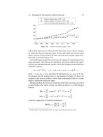
Figure 4.1. The price series for Scottish and Norwegian salmon sold in the United King-
dom (MH: Marine Harvest Scotland Ltd, which is Nutreco’s salmon farming operation in
Scotland). Source: Figure 4.7 (Competition Commission 2000). The CC, in turn, describes
the source as a Lexecon report provided during the investigation.
particular, Norwegian farmed salmon.
11
Both salmons are Atlantic salmons but it
was unclear whether buyers in the United Kingdom actually had sufficiently similar
tastes for the different types of salmon to treat the market as the market for Atlantic
salmon sold in the United Kingdom rather than, for example, the market for Scottish
salmon sold in the United Kingdom.
Figure 4.1 plots the price series for each of Scottish and Norwegian farmed
salmon.
Calculating the correlation coefficient between the price series gives us the result
of 0.67. (See appendix 4.4 of the CC report.) Clearly, this figure is more difficult to
interpret compared with the result of 0.90 obtained in the previous example. Such
situations provide us with a difficult question: clearly, the correlation is positive but
is the correlation high enough to suggest these two products are in the same market?
In the salmon case, the consultants suggested a “comparability” test that involved
comparing the figure obtained with the correlation coefficients of clear substitutes
in that market. This seems a very sensible practical approach, though one which
introduces some room for flexibility in choosing the comparison. In this case the
consultants chose to compare the correlation coefficients with those obtained by
comparing U.K. prices of salmon of different weights. The results are presented in
table 4.4.
11
See the U.K. CompetitionCommission’sreport“Nutreco Holding NV and HydroSeafoodGSP Ltd:A
report on the proposed merger” (2000). See www.competition-commission.org.uk/inquiries/completed/
2000/index.htm. The CC subsequently revisited salmon in the proposed merger of Pan Fish and Marine

Harvest in 2006. See www.competition-commission.org.uk/inquiries/ref2006/panfish/index.htm.
174 4. Market Definition
Table 4.4. Correlation between MH U.K. prices for various weight categories.
2–3 kg 3–4 kg 4–5 kg
2–3 kg 1.00 — —
3–4 kg 0.76 1.00 —
4–5 kg 0.52 0.87 100
Source: Lexecon. Table 1 (Competition Commission 2000). The CC, in turn, describes the source as a
Lexecon report provided during the investigation.
In this case, 0.67 is slightly lower than the price correlation coefficient obtained
for adjacent weight cells but higher than the coefficient obtained for salmon two
weight cells apart.
Besides looking at the coefficient itself, the graph of the series allows a visual
inspection and it is pretty clear that the two prices are at least somewhat correlated.
There is a similar pattern over time both in the level of the prices (the two series are
pretty much on top of one another) and also in the way the two series move together
with at least some shocks appear to broadly coincide in timing. Naturally, one needs
to be rather careful in drawing hasty conclusions from an apparent correlation (visual
or numerical) such as these ones. In the next sections we explain why a superficial
correlation analysis can go wrong and how not to fall into the most common traps
in using price correlations for market definition.
4.2.3 Use and Limitations of Price Correlation Analysis
In order to understand what lies behind price correlations, we need to understand
what lies behind the prices of two differentiated products.
12
The prices of products
are determined by the costs incurred in their production, the level of the demand they
face, and by the availability and prices of substitutes. When we use price correlations
to determine whether two goods are in the same market, we are assuming that what
determines the co-movement in prices is primarily the influence of differences in the

goods’ prices on consumer behavior. However, there are other factors, unrelated to
consumer substitution between products, which can cause a co-movement and there-
fore produce a positive correlation in prices. In particular, cost factors may co-move
while correlated demand shocks and trends may also produce a false impression that
prices are affecting each other. We discuss each of these alternative scenarios below.
Consider a situation where the demand for two differentiated products is captured
by the two linear demand equations expressed as
q
1
D a
1
 b
11
p
1
C b
12
p
2
and q
2
D a
2
 b
22
p
2
C b
21
p

1
:
Assuming each product is produced by a different firm which respectively maximize
12
For a critique of the use of price correlation analysis, see, for example, Werden and Froeb (1993a).
A response is provided by Sherwin (1993).
4.2. Price Level Differences and Price Correlations 175
profits and compete in prices, we can calculate each firm’s reaction function and
then we can solve for the Nash equilibrium in prices as the solution to the two reac-
tion function equations. Specifically, under price-setting competition, we showed in
chapter 1 that the reaction functions of the firms will be
p
1
D
c
1
2
C
a
1
C b
12
p
2
2b
11
and p
2
D
c

2
2
C
a
2
C b
21
p
1
2b
11
;
where c
1
and c
2
are the marginal costs of goods 1 and 2 respectively. After some
algebra, Nash equilibrium prices are described by the following formulas:
p
NE
1
D
Â
4b
11
b
22
4b
11
b

22
 b
12
b
21
ÃÂ
c
1
2
C
a
1
2b
11
C
b
12
4b
11
Â
c
2
C
a
2
b
22
ÃÃ
;
p

NE
2
D
Â
4b
11
b
22
4b
11
b
22
 b
12
b
21
ÃÂ
c
2
2
C
a
2
2b
22
C
b
21
4b
22

Â
c
1
C
a
1
b
11
ÃÃ
:
First note that the prices depend on the intercepts of the demand equations (a
1
and
a
2
), the own-price effects (b
11
and b
22
), and the cross-price effects (b
12
and b
21
).
They also depend on the cost of both goods.
Suppose b
12
D b
21
D 0 so that the products are completely unrelated in terms

of demand substitutability. The formulas for the Nash equilibrium prices reduce to
p
NE
1
D
c
1
2
C
a
1
2b
11
and p
NE
2
D
c
2
2
C
a
2
2b
22
:
Note that from these expressions we can see that there are several ways in which
we can find positive price correlations even though the products are not related on
the demand side and are not substitutes.
4.2.3.1 False Positives: Correlated Inputs or Demand Shocks

If two products use the same input and its price varies, we will generate a positive
correlation in the costs of producing the two products. For instance, both airline
travel and rubber are intensive in fuel-based inputs. As the price of oil varies, the
costs of producing both airline travel and rubber will covary so that cov.c
1
;c
2
/ ¤ 0.
Moreover, the equations above capture the intuition that prices vary with marginal
costs and so the prices of the outputs, airline travel and rubber, will also be correlated.
A (in this case very) naive application of price correlation analysis might therefore
find that the prices of rubber and airline travel are correlated and thus argue they are
in the same product market. Naturally, such a conclusion would be a mistake—the
positive correlation is a “false positive” for market definition since we are not in
truth learning from the positive correlation in prices that the products are demand
substitutes. Putting it another way one could not plausibly claim that airline travel
is a demand substitute for rubber, that if the price of rubber were to go up, people
would increase their air travel!
176 4. Market Definition
Jul-95
Oct-95
Jan-96
Apr-96
Jul-96
Oct-96
Jan-97
Apr-97
Jul-97
Oct-97
Jan-98

Apr-98
Jul-98
Oct-98
Jan-99
Apr-99
Jul-99
Oct-99
Jan-00
Apr-00
Feed (relative price)
0.06
0.07
0.08
0.09
0.10
Exchan
g
e rate £/NOK
0.8
0.9
1.0
1.1
1.2
1.3
1.4
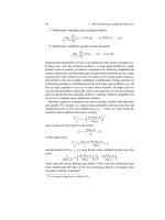
Figure 4.2. Ratio of U.K. to Norwegian feed prices.
Source: U.K. Competition Commission salmon report.
In the “salmon debate” the U.K. Competition Commission (CC) made an attempt
to exclude the risk of false positives due to the positive correlation in costs potentially
induced by common input prices. In particular, salmon feed may be sold in a global

market. If so, then the marginal costs of producing salmon in the United Kingdom
and in Norway may positively co-move even if the two products are not in truth
demand substitutes. To test this hypothesis the CC looked at the relative prices of
salmon feed in Norway and the United Kingdom. Doing so makes it clear that the
cost of feed in the United Kingdom was falling with respect to the cost of feed in
Norway during the period considered.
Figure 4.2 makes it clear that while the positive correlation observed in the price
data could be explained by a positive correlation in costs, in this case costs appear
to be negatively correlated and so this potential false positive explanation is not
supported by the facts.
A related cause of false positives in a price correlation exercise is the occurrence
of common demand shocks, when cov.a
1
;a
2
/ ¤ 0. To see why, consider any two
normal goods, say cars and holidays. When the economy is good we will tend to see
high demand, and hence high prices, for both cars and holidays and yet, of course,
we would not want to define those two goods as being in the same market. Income
is one demand shifter that may show up in common price movements but, of course,
there are potentially many others, each of which is a danger for generating a false
positive between prices of goods which experience the same demand shifters rather
than are demand substitutes. Unsurprisingly, in many cases there will be room for
substantial debate about the implications of a positive correlation.
4.2.3.2 Spurious Correlation and Nonstationarity
Another problem which emerges as a term in the debate around price correlations
when measuring them with time series is that commonly termed “spurious correla-
tion.” Spurious correlation occurs when two series appear to be correlated but are in
4.2. Price Level Differences and Price Correlations 177
fact only correlated because each of them has a trend. The correlation in this case is

a “coincidence” and is not the product of any genuine interrelation between the two
products. This idea was explored in Yule (1926), who showed that the correlation
coefficient actually converges toward 1, i.e., perfect correlation, for any two time
series that each respectively has an upward trend. Similarly, if one series trends
upward while the other trends down, we will find a correlation that tends to 1.
These facts can lead to some serious inference problems. For example, the num-
ber of pirates over the Atlantic has decreased over the last three centuries while
the average height of individuals has increased. These would be two variables that
would trend in opposite directions and so, given a long enough time series we would
find high levels of negative correlation between the two. As the number of pirates
decreased the average height increased, but of course it would be nonsense to argue
that the decrease in the number of pirates has anything to do with the increase in
the average height of the population.
13
The basic lesson is that one needs to be
very careful when dealing with correlations when variables trend. Seemingly highly
robust correlations can be completely spurious and the two variables may be in fact
completely unrelated.
A formal way to approach this problem is to assess whether a series is “station-
ary.”
14
A series is stationary when, eventually, shocks to the series no longer affect
the value of the series.
15
As the simplest example, suppose the series at each point
in time is entirely independent of the points in any other time period. In that case, if
we know the value of the variable yesterday or the day before, this carries absolutely
no information for predicting the value of the variable today. And, in particular, if
a shock occurs, it is not at all persistent: in the next period there is absolutely no
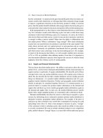
trace of it. This archetype stationary series is called a form of “white noise.” As a

concrete example, define "
t
 UniformŒ1; 1 to be a variable that in each period
takes a value randomly between 1 and 1 according to a uniform distribution. The
time series produced by such a data-generating process will look like figure 4.3.
13
Yule’s original example reported a correlation of 0.95 between the proportion of marriages performed
by the Church of England and the mortality rate over the period 1866–1911. The assumption is that the
relationship between these two series is not causal—a stance which all but the most ardent of religious
conspiracy theorists would probably accept. Granger and Newbold (1974) make a similar point but in
the context of “random walks.”
14
For an introduction to nonstationarity see the guide developed when Robert Engle and Clive Granger
won the Nobel Prize in Economics partly for their work in this area, available at />nobel
prizes/economics/laureates/2003/ecoadv.pdf. There are also numerous textbooks in this area (see,
for example, Stock andWatson (2006) or, for a moreadvanced discussion, Banerjeeet al. (2003), Johansen
(1995), and Hendry (1995)).
15
Formally, a stationary process is a stochastic process whose probability distribution at any
fixed point in time does not change over time. That is, if the joint distribution of a time series
.X
1Cs
;X
2Cs
;:::;X
T Cs
/ does not depend on s. That means we can observe a time series of any
length T and the date at which we start observing it will not affect the joint distribution of the data. This
property is sometimes known as “strict” stationarity and other forms of stationarity are also possible. For
example, we may only require that the first and second moments of the series do not vary over time and

this would be a weaker form of stationarity.
178 4. Market Definition
1.5
1.0
0.5
0
−0.5
−1.0
−1.5
0 50 100 150
200
Figure 4.3. White noise series:  D 0.
Now consider a price series generated by the first-order autoregressive series,
P
t
D P
t1
C"
t
, where we might again suppose that "
t
 UniformŒ1; 1. In this
case, today’s price is determined by the price in the previous period and a “white
noise” shock. It is interesting to see the extent to which the shocks persist in such a
series. To do so, substitute in the expression for prices successively to give
P
t
D P
t1
C "

t
D .P
t2
C "
t1
/ C "
t
D 
2
P
t2
C "
t1
C "
t
D 
2
.P
t3
C "
t2
/ C "
t1
C "
t
D 
3
P
t3
C 

2
"
t2
C "
t1
C "
t
;
P
t
D 
t
P
0
C 
t1
"
1
CC"
t1
C "
t
:
Doing so allows us to see that prices today are determined by the price at the begin-
ning of the series, the initial condition, and then all of the shocks that subsequently
happened weighted by terms that depend on the parameter .If<1, the effects
of both the initial condition P
0
and also all the old shocks die out with time. The
smaller the , the faster the effect of the shock dies out, i.e., the less persistent the

shocks are. When this happens we say that the series is stationary. In contrast, note
that if  D 1, then shocks to the series will never stop mattering, they will always
matter to the value of prices being observed no matter how much time passes. In
that case, we say that the shocks are persistent as the past never goes away, always
affecting the current value of the price. If  D 1, we say that the price series follows
a “random walk” and such a series is an example of an integrated or a nonstationary
process. If a series is integrated of order 1, it means that the first difference of the
series, the series P
t
P
t1
, is stationary. An example of integrated time series and
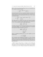
also a number of stationary time series are shown in figure 4.4, which presents an
integrated series which puts  D 1 and three other, stationary, time series which
respectively set  equal to 0, 0.5, and 0.8.
Unlike the stationary time series, the integrated time series tends to wander off and
does not quickly revert to its long-run value. To see why, note that a UniformŒ1; 1
variable will always have a mean zero and so the series will never appear to wander
4.2. Price Level Differences and Price Correlations 179
−4
−2
0
2
4
6
8
10
12
14
16

0 20 40 60 80 100 120 140 160 180 200
= 0
= 1
= 0.8
= 0.5
ρ
ρ
ρ
ρ
Figure 4.4. Examples of an integrated and a number of stationary time series.
away from that average.A stationary series can wander off a little from the mean, but
eventually the past stops mattering and so the behavior of the series between, say,
periods 0 and 100 cannot be very different from that between periods 100 and 200. In
contrast, an integrated time series has no such mean-reversionary tendency. It turns
out that if we have two price series generated with  D 1, even if the shocks in each
series are entirely independent of one another, we will find that cov.P
1
t
;P
2
t
/ !˙1
in a fashion that is highly reminiscent of the results we saw when variables have
trends. Thus, in the presence of integrated time series we face an additional danger
that we will find highly correlated prices but that the correlation will be entirely
spurious.
The salmon example provides an illustration of the kinds of debates that some-
times arise in competition cases. Consider figure 4.5, which plots the U.K. spot
market prices for salmon produced in the United Kingdom and in Norway. Note in
particular that up to about the year 2000, the time series appear to be characterized

by a number of short-term shocks which do not look as though they persist for very
long, if at all. Note, for example, the big spikes which last for just one period. In
addition, the series behave like stationary series oscillating around their mean val-
ues. In contrast, after the year 2000, the series seem to both wander away from their
previous mean and so appear to the eye more like nonstationary processes. If the
correlations obtained previously are driven by this part of the data, then our result
might not be reliable, that is, if the correlation coefficient for this section of the time
series is driven purely by spurious correlation. One potential response is to split the
sample and calculate the correlation on the first—stationary—section of the data.
Another response is to look at whether two prices are tied together by examining
the stationarity of the ratio of prices. Suppose that economic forces ensure that two
prices are never too different from one another for long periods of time because
supply or demand substitutability forces the “law of one price” to broadly hold.
Then we might expect to find that the relative prices for products should have the
180 4. Market Definition
2.00
2.20
2.40
2.60
2.80
3.00
3.20
1997w27
1997w32
1997w37
1997w42
1997w47
1997w52
1998w5
1998w10

1998w15
1998w20
1998w25
1998w30
1998w35
1998w40
1998w45
1998w50
1999w3
1999w8
1999w13
1999w18
1999w23
1999w28
1999w33
1999w38
1999w43
1999w48
2000w1
2000w6
2000w11
2000w16
2000w21
2000w26
2000w31
Price (£/kg)
Estimated price of Norwegian salmon in U.K.
MH ‘‘uncontracted’’ price in U.K.
Stationary
Nonstationary

Figure 4.5. Stationary and nonstationary segments of price series.
Source: U.K. Competition Commission salmon report. Original source: Lexecon.
0.8
0.9
1.0
1.1
1.2
Relative price
w27 97 w27 98 w27 99 w27 00
Date
Figure 4.6. Relative prices. Source: U.K. Competition Commission
salmon report. Original source: Lexecon.
long-run reversionary property, i.e., they should be stationary. Using the price series
of our salmon example above, define P
Scottish
t
=P
Norwegian
t
D 
t
, which is graphed in
figure 4.6.
A first look seems to indicate that in the first few periods, the price of Scottish
salmon is appreciating over time with respect to the price of Norwegian salmon,
indicating that they may not be perfect substitutes. For the rest of the sample the
ratio generally varies above 1. The claim that the relative price ratio of two goods
should be stationary when they are demand substitutes appears plausible but it is in
fact a very strong claim. Let us look at its theoretical foundation.
4.2. Price Level Differences and Price Correlations 181

Recall the differentiated product Nash equilibrium in prices defined at the
beginning of this section described the ratio of Nash prices as
p
NE
1
p
NE
2
D
Â
4b
11
b
22
4b
11
b
22
 b
12
b
21
ÃÂ
c
1
2
C
a
1
2b

11
C
b
12
4b
11
Â
c
2
C
a
2
b
22
ÃÃ
ÄÂ
4b
11
b
22
4b
11
b
22
 b
12
b
21
ÃÂ
c

2
2
C
a
2
2b
22
C
b
21
4b
22
Â
c
1
C
a
1
b
11
ÃÃ
D
Â
c
1
2
C
a
1
2b

11
C
b
12
4b
11
Â
c
2
C
a
2
b
22
ÃÃ
Â
c
2
2
C
a
2
2b
22
C
b
21
4b
22
Â

c
1
C
a
1
b
11
ÃÃ
‹
D v
t
;
where the question mark indicates that we are testing whether the ratio generates a
stationary process. Note in particular that p
NE
1
=p
NE
2
can be stationary, but only under
very stringent conditions. In particular, note that even if the products are substitutes,
the relative costs of the two products need to remain broadly constant, as will the
relative demand intercepts and the own- and cross-price elasticities. Each of these
will need to stay broadly constant over the period examined, or somehow fortuitously
move together, or else relative prices will not appear as a mean-reverting stationary
series. If, for example, we have a persistent shock in cost or demand for one of the
products only, we might wrongly conclude that the products are not related.
On the other hand, even if the products are not demand substitutes, so that b
ij
D 0

for i ¤ j , we could potentially wrongly find stationarity in relative prices when
common shocks to costs or demand for the two products appropriately cancel each
other out or indeed are themselves stationary.
All that said, when the goods are perfect substitutes, we do expect the “law
of one price” to hold and that should act to keep the prices of the two products
approximately the same. That is pretty strong intuition, but the lesson of this section
is that price correlation exercises are not for the naive and certainly cannot be applied
as though they are a panacea for market definition. In this chapter we have seen
that lesson a number of times, and here we see again that (1) rejecting stationarity
does not imply that the goods are not substitutes and (2) accepting stationarity
does not necessarily imply that goods are demand substitutes even with seemingly
high correlation coefficients. In general, we will want to substantiate claims about
stationarity and correlations by checking what happened to the costs of, and demand
for, the products during the period of interest. If such shocks exist they may cause
a false negative if only one product is affected and substitution is less than perfect.
If the shocks are common to both products, they may cause a false positive and the
products can appear to be more related than they really are.
182 4. Market Definition
There are several ways in which one can test the existence of stationarity. The first,
illustrated in Stigler and Sherwin (1985), looks at the correlation in price changes,
i.e., the correlation in the first differences of prices:
Corr.P
1
t
 P
1
t1
;P
2
t

 P
2
t1
/:
An alternative method is to statistically test whether nonstationarity might be a
problem. To do so we can compute a test called the Dickey–Fuller test for each
price series to see whether each price series is nonstationary. Then we use the same
test to see whether the relative prices are stationary. If the hypotheses that the two
individual series are stationary are rejected but the relative price series does appear
stationary, then we can claim that the result is consistent with a connection between
the markets which suggests the two products should be in the same market in a way
akin to getting correlation in the levels of stationary price series. Of course, whether
stationary or nonstationary, correlation analysis runs the substantial risk of false
positives or negatives and as a result it is usually a mistake to simply calculate the
correlation and accept it at face value as strong evidence about market definition.
We end this section by noting that there is a more formal econometric approach
to the question of testing for co-movement in prices which involves testing for
“co-integration.” This type of analysis involves both complex and sometimes sub-
tle econometric arguments and also is often applied in a way that is insufficiently
informed by economic theory. The combination can be extremely dangerous. For
example, one result which, on the face of it, suggests that researchers do not need
to worry about endogeneity when working with co-integrated series is the result
that says OLS estimators of “co-integrating” relations are “superconsistent” and
integrated regressors can be correlated with error terms (see Stock 1987). Naive
applications of that result argue, for example, that it implies that it is unproblematic
to run regressions of price on quantity. Such claims are obviously both dangerous
and ultimately “wrong,” since, for example, you still would not know whether your
regression were a demand or a supply curve.
16
While in principle, under special

circumstances, you may not have an endogeneity problem, you certainly will not
have escaped the fundamental identification problem that both supply and demand
curves depend on prices and quantities. Investigators with limited knowledge in the
co-integration arena are therefore advised to proceed with extreme caution when
attempting to apply complex econometric arguments with sometimes subtle impli-
cations. The risk of being led seriously astray by apparently extremely attractive
16
Engle and Granger (1987) studied a single “co-integrating” relationship and showed that applying
OLS to a regression of the form Y
t
D ˛X
t
C "
t
, where Y and X are integrated (of order 1) and
"
t
is stationary gives us a “superconsistent” estimator of ˛. The terminology of “superconsistent” is
used to indicate that the estimator is consistent and converges to the true parameter value faster than a
normal OLS estimator (at rate T instead of at rate T
1=2
). OLS estimators use the correlation EŒX
t
"
t

to identify the parameter ˛ and the superconsistency result occurs because X
t
is integrated while "
t

is
stationary so that intuitively the correlation between them will necessarily be small because X wanders
away from its initial value while "
t
mean reverts.
4.2. Price Level Differences and Price Correlations 183
econometric theorems is very high. On the other hand, if carefully applied with
both economic and econometric theory solidly in mind when doing so, the tools for
dealing with integrated and co-integrated time series can sometimes help avoid the
problem of spurious correlation.
17
4.2.3.3 The Risk of False Negatives
We have already illustrated how, in a world of imperfect substitutes, asymmetric
shocks to demand and costs can cause price series to deviate from one another even
when the products are perhaps even fairly close substitutes. We close this section by
noting that there are other circumstances when we will underestimate the degree of
substitutability of two products by just looking at how their prices move together.
In particular, if the signal-to-noise ratio is low, we will find little correlation
between the prices but this result will be driven by random short-lived shocks to
the prices of the product and the apparent lack of correlation will not reflect the
underlying structural relationship between the products. For instance, suppose the
inputs are really different for the two goods and input prices move around a lot.
Then the observed correlation in prices will be small due to the variance in the price
series caused by shocks to input prices even though the two series may exhibit some
limited co-movement. Also, if the data are noisy due to poor quality or measurement
problems and the actual prices do not vary muchin the period observe, the correlation
coefficient will appear small since it will only pick up the noise in the series. When
the size of the shocks is large relative to the movement of the price series over the
period observed, this problem will be exacerbated since the “signal to noise” ratio
will be low.

Similarly, the picture generated by contemporaneous correlations in prices may
mislead investigators when, for example, prices respond to changes in market con-
ditions only with a time lag. Even if two products are in fact good long- or medium-
term demand substitutes, we may see little contemporaneous correlation in prices
and wrongly conclude that the products are not related.
4.2.4 Rival Cost and Demand Data for Price Correlation Analysis
As in all quantitative analysis, one cannot draw more information from the analysis
than is already present in the data. If the data are noisy, we will find a low level of
17
These tools are particularly important andpopular in macroeconomics,butnot without critics(see, for
example, Greenslade and Hall 2002). Those authors argue that “in a common realistic modeling situation
of limited data set and the theory requirements of a fairly rich model, the techniques proposed in the
existing literature are almost impossible to implement successfully.” That quote gives a more pessimistic
impression than those authors in fact conclude with, when these tools are appropriately combined with
economic theory, but it should nonetheless provide a very useful cautionary note to any investigator.
Difficulties of identification, the way in which purely statistical analysis must be supplemented with
economic theory, and the appropriate framework for statistical analysis are certainly not unique to the
co-integration literature—they are each generic difficulties that must be faced and overcome in any
serious econometric analysis.
184 4. Market Definition
correlation no matter how related the products really are. If visual inspection shows
that the prices co-move, the correlation coefficient will tell you that the prices co-
move, although you might derive some additional information about the scale of the
co-movement from the number itself and are likely to want to consider the statistical
significance of any correlation.
18
Whatever the numerical value of the correlation,
a central lesson we have attempted to hammer home is that it can be very important
to get underneath the number to identify the source of the co-movement.
In this section we outline a “test” for identifying good sources of co-movement

in prices. This test consists of identifying changes in the demand or cost of the
potential substitute product that do not affect the original product. This could be
changes in the price of an input (i.e., cost movement) used in the substitute product
only or a change in the intensity of demand by a group of users that do not want
the original product. These changes are likely to affect the price of the potential
substitute. Noticing an impact on the price of the original product would indicate
that the two are indeed substitutes enough to influence each other’s prices.
To see why, recall that economic theory predicts different price-setting mecha-
nisms for prices when in the presence or absence of a substitute. In particular, the
expressions for Nash equilibrium prices that we obtained in those two cases were
respectively
p
NE
1
D
Â
4b
11
b
22
4b
11
b
22
 b
12
b
21
ÃÂ
c

1
2
C
a
1
2b
11
C
b
12
4b
11
Â
c
2
C
a
2
b
22
ÃÃ
and
p
NE
1
D
c
1
2
C

a
1
2b
11
:
When analyzing price correlations, we are often interested in knowing whether b
12
is nonzero. Examining these formulas, it is apparent that a good way to test for such
connections is to observe shifts in the other product’s demand or costs (a
2
or c
2
)
provided that variation is not of the form that would contemporaneously shift the
product’s own demand or cost (a
1
or c
1
). If the effect of such a shift is noticeable
in p
1
, then we will be able to conclude that b
12
is nonzero, though as with any
price correlation analysis it will nonetheless be difficult to decide whether or not
b
12
is truly big enough to justify putting both products in the same market. As with
many areas of competition policy, ultimately the decision-making body (regulator,
18

As we have already mentioned, statistical inference with nonstationary time series data is “nonstan-
dard” in the sense that t-statistics of 2 are generally not enough to establish statistical significance. In fact,
while we can, for example, still calculate correlations, R-squared, and t-tests, they often will not have
the distributions we usually expect them to have. For example, we can calculate a t-test but the statistic
we calculate will not have a “t”-distribution when our data set involves integrated time series. In practical
terms, while we usually use a t -value of 2 to evaluate statistical significance (difference from zero with
95% significance), the correct critical values will typically be higher, and sometimes far higher (perhaps
5 or 10 instead of 2). See, for example, the critical values provided for tests of “integration” provided
by Dickey and Fuller (1979). Other related popular tests for nonstationarity include the “augmented
Dickey–Fuller” test and the Phillips–Perron test.
4.3. Natural Experiments 185
competition authority, or court) will need to make a judgment taking into account all
of the various pieces of evidence including price correlation evidence on the correct
market definition.
4.3 Natural Experiments
Price correlation analysis is a method we can use to attempt to estimate the degree
of substitutability between two products by estimating the extent to which two
products’ prices move systematically together. On the one hand, price correlations
provide rather indirect evidence compared, for example, with attempts to evaluate
the cross-price elasticity of demand between two products. On the other hand, the
method is simple and in particular far simpler than having to actually estimate a
demand function. Natural experiments or “shock analysis,” when applied to prices,
follow a similar logic but are far more careful at the outset to control the source of the
variation in the data that we use to identify substitutability. Rather than evaluating
the correlation and then checking explanations for its source, shock analysis looks at
the reaction of the price(s) of other goods following an exogenous shock on the price
of one good, the one at the center of the investigation. Shock analysis is the simplest
way of getting a feel for the magnitude of own- and cross-price elasticities of demand
without getting involved in a more complex econometric analysis. Whenever there
is a possibility to properly conduct a shock analysis, this method will be helpful

since it is both simple to apply and often very informative, making it a powerful
technique. Of course, the investigator does nonetheless need to be very careful to
ensure that the “shock” causing the initial price shift is genuinely exogenous and
not determined by market conditions affecting consumers or competitors.
4.3.1 Informative Exogenous Shocks
To see the logic of natural experiments, assume a sudden unanticipated exogenous
decrease in the price of a good A, P
A
, such as that illustrated in figure 4.7. Such a
change may occur, for example, by design, perhaps if a firm conducts a marketing
experiment in an attempt to learn about the sensitivity of demand to its price. An
exogenous change in the price of goodA may feed through into (1) the price of good
B, (2) the quantity of good B, and (3) the quantity of good A.
Once the observed exogenous change in P
A
occurs, we can simply look at the
subsequent changes in Q
A
and Q
B
to obtain the own- and cross-price elasticities of
demand. If the reaction to a decrease of P
A
is a sharp increase of Q
A
and a sharp
decrease of Q
B
, then we can confidently assert that A and B are demand substitutes.
More closely related to the price-correlation analysis we studied previously, the

price decrease in A may lead us to observe a reduction in the price of B. Ideally, an
investigation would have data on all the prices and quantities, but the reality is that
data sets may frequently be incomplete, with perhaps just the price data available.
186 4. Market Definition
Shock
P
1
P
2
Good A Good B
P
1
P
2
Q
1
Q
2
Q
2
Q
1
MR
2
MR
1
MC
B
D
2

(P
2
)
D
2
(P
1
)
Shock
A
A
AA
B
B
B
B
B
B
A
A
Figure 4.7. Effect of a shock in the price of a good on another good.
A key factor for the success of the methodology is the fact that the original shock
on prices is exogenous and not related to the demand of either product A or B, nor
related to the cost of inputs for B. It is unfortunately not always easy to find such
situations, although opportunities for shock analysis do occur.
A practical example is provided by the decision in 1996 by a cinema in New
Haven, Connecticut, to lower the prices of its evening adult admission ticket to
newly released films to just $5 for a three-week period. Such an unusual move was
heavily reported by the local newspapers. Given such a move, it enables us to look
at the response of the theaters near to the venue which lowered its price.

19
Cinemas
are in the same geographical market if moviegoers consider them as alternatives.
One can easily imagine someone deciding on a movie by checking the shows in a
group of cinemas where she could consider going. If one cinema becomes cheaper,
this person might be more likely to attend that cinema, particularly if the movie
shown is the same as the ones shown elsewhere. If cinemas compete for customers,
then there is an incentive by competing cinemas to also reduce their prices (or show
sufficiently unique and attractive movies). Observing the reaction of the cinemas in
an area after a unilateral price decrease by one of them can therefore be a good way
to determine which cinemas are likely to be competing for the same audience.
There were five cinemas in the New Haven area located around the cinema which
cut prices (the Branford 12), as shown in figure 4.8.
The pricing responses of the rival theaters are reported in table 4.5.All the cinemas
except for theYork Square cinema (number 3) showed first-run, i.e., newly released,
films.
Table 4.5 provides useful information about both geographic market definition
and also product market definition. First consider geographic market definition.
Note that the two closest cinemas showing popular films responded with similar
19
As we have already noted, exogenous data variation is useful for estimating demand as well. The
price and also sales data from this experiment were collected and used in Davis (2002).
4.3. Natural Experiments 187
Orange
North Haven
New Haven
Branford
Milford
I95
I95

I91
2
4
3
1
5a,b
Figure 4.8. Map of locations of cinemas involved in the experiment. The theater
labeled “4” was the Branford 12 screen cinema whose price was cut for three weeks.
Table 4.5. Theater pricing responses to the pricing
experiment performed by the Branford 12 cinemas.
Pricing strategy/
Theater Chain response
1 Showcase Orange National Amusements $4.50 for three weeks
2 Showcase North Haven 8 National Amusements $4.50 for three weeks
3 York Square (art house) Independent No change
4 Branford 12 HOYTS $5 for three weeks
5a Showcase Milford 5 National Amusements No change
5b Milford Quad National Amusements No change
Source: Davis (2002).
price changes while the more distant ones did not. Both the Showcase Orange and
the Showcase North Haven responded by decreasing their prices to $4.50, which,
as an aside, also provides a nice example that committing to prices provides your
rivals with a second mover advantage to undercut you. The two theaters in Milford
(denoted as 5a,b in the table and on the map) could have reacted to the change in
price initiated by the Branford 12 but they did not and that fact is consistent with
those theaters being outside the geographic market appropriate for the Branford 12.
On the other hand, it is perhaps more surprising on the face of it that they did not
respond to the somewhat closer theater’s price, particularly the Showcase Orange,
labeled 1 on the map. Since the Showcase Orange theater belongs to the same chain
as those in Milford (National Amusements), the incentives to further propagate the

price reduction down along the coastline are greatly mitigated. The revenue loss of
NationalAmusements cinemas due the lower price at cinemas 1 and 2 were probably