Mechatronic Systems Applications Part 12 ppt
Bạn đang xem bản rút gọn của tài liệu. Xem và tải ngay bản đầy đủ của tài liệu tại đây (1.45 MB, 20 trang )
PalletizingSimulatorUsingOptimizedPatternandTrajectoryGenerationAlgorithm 285
T
h
(
L
W
ch
o
Fi
g
2.
3
2.
3
T
h
pa
h
o
Fi
g
(1
)
(2
)
(3
)
ed
2.
3
A
s
in
i
fo
u
h
is case involves
4
L
,
4
W
) and resi
z
2
W
and
3
W
. Then
,
o
sen (Fi
g
. 4.).
g
. 4. Treatment o
f
3
The Fast Algo
r
3
.1 Definition
h
e Fast al
g
orith
m
tterns. In additi
o
o
le in the followi
n
g
. 5. Treatment o
f
)
In the first met
h
)
In the second m
e
)
In the third me
t
g
e.
3
.2 Schematic D
s
this al
g
orithm
d
i
tial solutions of
t
u
r parameters (F
i
the second phas
z
es
1
L
and
2
L
,
a
,
the first and s
e
f
Steudel’s al
g
ori
t
r
ithm
m
has similar pr
o
o
n, Treatment 3 i
s
ng
three methods
f
the Fast al
g
orit
h
h
od, the boxes ar
e
e
thod, the boxes
t
hod, the boxes
a
iagram of the F
a
d
oes not conside
r
t
he first phase fi
n
ig
. 6.).
e. In the second
a
nd Treatment 2
f
e
cond methods a
r
t
hm
o
cesses with wh
i
s
adapted to app
l
so as to remove
t
h
m
e
cut b
y
the two
h
are cut b
y
the t
w
a
re cut b
y
the lef
t
a
st Algorithm
r
all block sizes, i
t
n
d the combinati
o
phase, Treatme
n
f
ixes (
1
L
,
1
W
) an
r
e compared an
d
i
ch to
g
enerate t
h
ly
the heuristic r
e
t
he overlapped a
r
h
orizontal ed
g
es
o
o vertical ed
g
es.
t
vertical ed
g
e a
n
t
has a more rap
i
o
n rather than u
s
n
t 1 fixes (
3
L
,
3
W
d (
4
L
,
4
W
) and
r
d
the better sol
u
h
e initial four s
o
e
cursivel
y
to the
c
r
ea (Fi
g
. 5.).
o
f the overlappe
d
n
d the lower hor
i
i
d calculation ti
m
s
in
g
DP, and def
i
3
W
) and
r
esizes
u
tion is
o
lution
c
entral
d
area.
i
zontal
m
e. The
i
ne the
Fig. 6. Parameters of the Fast algorithm
▪
a
: When maximizing the length of the block and disposing the boxes lengthwise, the
maximal possible number of boxes = 5l .
▪
a
: When maximizing the length of the block and disposing the boxes lengthwise, the
minimal possible number of boxes =
2l .
▪
b
: When maximizing the width of the block and disposing the boxes lengthwise, the
maximal possible number of boxes =
8w .
▪
b
: When maximizing the width of the block and disposing the boxes lengthwise, the
minimal possible number of boxes =
2w .
In the first phase, (
1
L
,
1
W
), such as ( , )a b , ( , )a b ,
( , )a b
, and
( , )a b
, are combined, and
(
1
L
,
1
W
), the width and length of the other blocks, can be determined.
1 1
2 2 4 4
( , ) ( , ) ,
L L W W
L W L W w l
w l
(1)
3 3 1 1
( , ) ( , )L W L W
(2)
After obtaining the four initial solutions in the first phase, these solutions are redefined by
applying the three treatments in the second phase.
Procedure FindBlockLayout(L,W,depth)
bestSolution 0
Find ,,, baa and
b
Make four initial Solutions.
i
s
(i=1,2,3, and 4), using them
MechatronicSystems,Applications286
For all
i
s
(i=1,2,3, and 4)
i
s
Number of boxes after the first treatment
i
s
Number of boxes after the second treatment
If max{
i
s
,
i
s
}>bestSolution, then
bestSolutionmax{
i
s
,
i
s
}
End If
If depth>>MaxDepth then
Return bestSolution
End If
For all central holes
i
s
Number of boxes in the area
excluding central hole
Let(
h
L
,
h
W
)=size of central hole
i
s
i
s
+FindBlockLayout(
h
L
,
h
W
,depth+1)
If
i
s
>bestSolution, then
bestSolution
i
s
End If
End For
End For
Return bestSolution
End Procedure
Algorithm SolvePLP(
wlWL ,,,
)
bestSolution0
For all(
wlWL ,,,
11
) that satisfy the inequality (2) or (3) and
wI
CWCL ,
11
Calculate all size of the five blocks
Call FindBlockLayout(
0,,
11
WL
) for all
i=1,2,3,4 and 5
If
5
1
)(
i
I
Bn
>bestSolution then
bestSolution
5
1
)(
i
I
Bn
End If
End For
End Algorithm
Fig. 7. The Fast algorithm
2.3.3 Computing Experience
The proposed algorithm was implemented in Visual C++ 6.0 and was compiled with the
maximized-speed option. This algorithm test generated a 2D pattern of boxes and its
calculation speed. As a hypothesis, the load balancing of a box and its stability were not
considered.
(L,W,l,w) Amount of boxes loaded
(1000,1000,205,159) 30
(1000,1000,200,150) 33
(22,16,5,3) 23
(30,22,7,4) 23
(14,10,3,2) 23
(53,51,9,7) 42
(34,23,5,4) 38
(87,47,7,6) 97
(1200,800,176,135) 38
(L: Length of Pallet, W: Width of Pallet, l: Length of Box, w: Width of Box)
Table 1. Test results of The Fast Algorithm (2D)
The above results were acquired by a computer with a K6-350-MHz CPU and 64MB RAM.
All problems were calculated within 1 s and resulted in optimal solution. To use this
algorithm practically, one dimension of height is applied additionally, and the 3D pallet
loading simulator is realized, as shown in Fig. 8.
Fig. 8. pattern generation S/W
3. Development of the 3D Robot Simulator
Several methods have been introduced to make industrial robots perform the palletizing
task. The first involved an online tutorial for the robot, which used a teach pendant to
enable the robot to mimic and memorize the worker’s motion. The second method is an
offline method that generates task data using a computer, and that downloads it onto the
robot controller. This chapter focused on offline task generation and simulation using a
PalletizingSimulatorUsingOptimizedPatternandTrajectoryGenerationAlgorithm 287
For all
i
s
(i=1,2,3, and 4)
i
s
Number of boxes after the first treatment
i
s
Number of boxes after the second treatment
If max{
i
s
,
i
s
}>bestSolution, then
bestSolutionmax{
i
s
,
i
s
}
End If
If depth>>MaxDepth then
Return bestSolution
End If
For all central holes
i
s
Number of boxes in the area
excluding central hole
Let(
h
L
,
h
W
)=size of central hole
i
s
i
s
+FindBlockLayout(
h
L
,
h
W
,depth+1)
If
i
s
>bestSolution, then
bestSolution
i
s
End If
End For
End For
Return bestSolution
End Procedure
Algorithm SolvePLP(
wlWL ,,,
)
bestSolution0
For all(
wlWL ,,,
11
) that satisfy the inequality (2) or (3) and
wI
CWCL
,
11
Calculate all size of the five blocks
Call FindBlockLayout(
0,,
11
WL
) for all
i=1,2,3,4 and 5
If
5
1
)(
i
I
Bn
>bestSolution then
bestSolution
5
1
)(
i
I
Bn
End If
End For
End Algorithm
Fig. 7. The Fast algorithm
2.3.3 Computing Experience
The proposed algorithm was implemented in Visual C++ 6.0 and was compiled with the
maximized-speed option. This algorithm test generated a 2D pattern of boxes and its
calculation speed. As a hypothesis, the load balancing of a box and its stability were not
considered.
(L,W,l,w) Amount of boxes loaded
(1000,1000,205,159) 30
(1000,1000,200,150) 33
(22,16,5,3) 23
(30,22,7,4) 23
(14,10,3,2) 23
(53,51,9,7) 42
(34,23,5,4) 38
(87,47,7,6) 97
(1200,800,176,135) 38
(L: Length of Pallet, W: Width of Pallet, l: Length of Box, w: Width of Box)
Table 1. Test results of The Fast Algorithm (2D)
The above results were acquired by a computer with a K6-350-MHz CPU and 64MB RAM.
All problems were calculated within 1 s and resulted in optimal solution. To use this
algorithm practically, one dimension of height is applied additionally, and the 3D pallet
loading simulator is realized, as shown in Fig. 8.
Fig. 8. pattern generation S/W
3. Development of the 3D Robot Simulator
Several methods have been introduced to make industrial robots perform the palletizing
task. The first involved an online tutorial for the robot, which used a teach pendant to
enable the robot to mimic and memorize the worker’s motion. The second method is an
offline method that generates task data using a computer, and that downloads it onto the
robot controller. This chapter focused on offline task generation and simulation using a
MechatronicSystems,Applications288
robot simulator. In this phase, the 3D robot simulator is presented based on the dimensional
data of a real target machine, the HX300, which is a six-axis industrial robot of Hyundai
Heavy Industrial Co. This robot model was realized by a commercial CAD modeler, and the
GUI was developed using OpenGL® and MFC of Microsoft Visual C++®. To solve and
analyze the forward and inverse kinematics equations, a general D-H parameter and the
Lagrangian dynamic equation were used. With this simulator, it was possible to compute
and display the joint torque, angle, and angular acceleration simultaneously. Fig. 9. shows
the realized 3D robot simulator that was developed using Microsoft Visual Studio® and
OpenGL®. It was possible to functionally calculate the velocity and acceleration of the
gripper and to simulate the user-defined motion. The coordinates, which are generated by
the pattern of loaded boxes on the pallet and the initial position of the box coming through
an in-feeder, are passed to the simulator, and using these coordinates, it was possible to
simulate the specified motion.
Fig. 9. Robot simulator for a palletizing task
4. C-Space and A* Algorithm for Trajectory Generation
4.1 C-Space Mapping of Obstacles
The palletizing task is generally composed of several palletizing components. These are
auxiliary but are nevertheless obstacles for the palletizing robot. The important part of this
study was to find the optimal path, considering the obstacles; hence, the concept of C-space
(Configuration Space) to solve this problem was applied. The configuration defined the
variables that exactly express the position and direction of an object, and the C-space
represented all of the spaces where configurations may be acquired. Using this concept, a
coordinate for each configuration was defined. In this coordinate, each point that was
approached by the robot gripper was expressed by joint angles (configuration, posture) of
the palletizing robot.
Fig.10. shows an example of the generation of the configuration space. First, on the basis of
the joint of the base frame, the imaginary plane was rotated 360 degrees like Fig.10.(a).
(a) Slice plane
(b) Apply the slice plane to the workspace to generate the C-space.
Fig. 10. Obstacles expressed in C-space
Step Task Layout C-space Enlarged Image
Elapsed
Time
(sec)
1
3.132
2
0.384
PalletizingSimulatorUsingOptimizedPatternandTrajectoryGenerationAlgorithm 289
robot simulator. In this phase, the 3D robot simulator is presented based on the dimensional
data of a real target machine, the HX300, which is a six-axis industrial robot of Hyundai
Heavy Industrial Co. This robot model was realized by a commercial CAD modeler, and the
GUI was developed using OpenGL® and MFC of Microsoft Visual C++®. To solve and
analyze the forward and inverse kinematics equations, a general D-H parameter and the
Lagrangian dynamic equation were used. With this simulator, it was possible to compute
and display the joint torque, angle, and angular acceleration simultaneously. Fig. 9. shows
the realized 3D robot simulator that was developed using Microsoft Visual Studio® and
OpenGL®. It was possible to functionally calculate the velocity and acceleration of the
gripper and to simulate the user-defined motion. The coordinates, which are generated by
the pattern of loaded boxes on the pallet and the initial position of the box coming through
an in-feeder, are passed to the simulator, and using these coordinates, it was possible to
simulate the specified motion.
Fig. 9. Robot simulator for a palletizing task
4. C-Space and A* Algorithm for Trajectory Generation
4.1 C-Space Mapping of Obstacles
The palletizing task is generally composed of several palletizing components. These are
auxiliary but are nevertheless obstacles for the palletizing robot. The important part of this
study was to find the optimal path, considering the obstacles; hence, the concept of C-space
(Configuration Space) to solve this problem was applied. The configuration defined the
variables that exactly express the position and direction of an object, and the C-space
represented all of the spaces where configurations may be acquired. Using this concept, a
coordinate for each configuration was defined. In this coordinate, each point that was
approached by the robot gripper was expressed by joint angles (configuration, posture) of
the palletizing robot.
Fig.10. shows an example of the generation of the configuration space. First, on the basis of
the joint of the base frame, the imaginary plane was rotated 360 degrees like Fig.10.(a).
(a) Slice plane
(b) Apply the slice plane to the workspace to generate the C-space.
Fig. 10. Obstacles expressed in C-space
Step Task Layout C-space Enlarged Image
Elapsed
Time
(sec)
1
3.132
2
0.384
MechatronicSystems,Applications290
Table 2. Palletizing Task Simulation and Generation of Optimal Trajectory using A*
Algorithm
In this progress plane, the objects surrounding the robot were scanned and the outline of a
section was generated. The left side of the Fig.10.(b) describes the specified palletizing task
layout. The outline, including its interior, could be considered an obstacle. In this study, the
outline was acquired by using an end effecter of the robot, and the free-movement and
obstacle zones in the C-space were generated as shown at the right side of Fig.10. To help
distinguish the 3D shape of C-space, various brightness and color are used. This figure is
necessary to generate the optimal path using the A* algorithm described in the next chapter.
4.2 Application of the A* Algorithm for Trajectory Generation
The A* method is a thorough, robust planning technique that determines either the
minimum cost path or whether no safe path exists. By exploring a map, the A* algorithm
generates nodes that are used to recode the current status. This technique is used to find the
optimal path between the gripping point (starting point) and the place’s down point (end
point). The original A* technique is outlined below. To begin, a 2D rectangular grid was
produced in which the cells were either safe or forbidden. The planning began at the starting
point, and the cells adjacent to this cell were probed. On the basis of a cost function, the cell
with the minimum cost was explored next. The cost function refers to the summation of
costs, which required one to move from the starting node to the current node, and the
“estimated” cost, which required one to move from the current node to the goal (a lineal
distance). Based on this algorithm, palletizing simulation is performed in the 3D space and
Table.2 is the results of the simulation.
5. Consideration of the Real Size of the Robot for Trajectory Generation
5.1 Modified Slice Plane (with horizontal thickness)
One of the disadvantages of the A* algorithm is the required computing time. The
aforementioned approach considers the robot arm as a bar. Hence, the computing time load
is relatively low. A real industrial robot, however, has an original volume, and these factors
3
12.267
4
9.734
have to be applied to the A* algorithm. The next step was to consider the real volume of the
robot when it scans obstacles and generates C-obstacles.
To do this, the slice planes were redefined because it was assumed that the original slice
plane had no thickness but that the modified slice plane had a thickness and that the factor
that changed the scanning point of an obstacle of each angle was a group of both sides of the
boundary of the modified slice plane (Fig. 11.). The thickness of the plane was determined
individually
by the thickness of the robot arm, including its gripper and load.
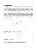
Fig. 11. Modified slice plane
5.2 Convex List and Graham’s Algorithm
Fig. 12. shows the scanning points that used the modified slice plane.
The proposed system used factors of convex list points of objects and the sum of half of the
thickness and a safe distance. As shown in Fig.12, the convex list was generated using the
inside apexes of objects and intersection points. If the number of intersection points was less
than two, the slice plane is regarded as meeting with one apex or edge.
Fig. 12. Convex list generation
Finally, Graham’s algorithm was used to generate the convex hull. This hull was used as the
new boundary of the object when the modified slice plane was applied.
PalletizingSimulatorUsingOptimizedPatternandTrajectoryGenerationAlgorithm 291
Table 2. Palletizing Task Simulation and Generation of Optimal Trajectory using A*
Algorithm
In this progress plane, the objects surrounding the robot were scanned and the outline of a
section was generated. The left side of the Fig.10.(b) describes the specified palletizing task
layout. The outline, including its interior, could be considered an obstacle. In this study, the
outline was acquired by using an end effecter of the robot, and the free-movement and
obstacle zones in the C-space were generated as shown at the right side of Fig.10. To help
distinguish the 3D shape of C-space, various brightness and color are used. This figure is
necessary to generate the optimal path using the A* algorithm described in the next chapter.
4.2 Application of the A* Algorithm for Trajectory Generation
The A* method is a thorough, robust planning technique that determines either the
minimum cost path or whether no safe path exists. By exploring a map, the A* algorithm
generates nodes that are used to recode the current status. This technique is used to find the
optimal path between the gripping point (starting point) and the place’s down point (end
point). The original A* technique is outlined below. To begin, a 2D rectangular grid was
produced in which the cells were either safe or forbidden. The planning began at the starting
point, and the cells adjacent to this cell were probed. On the basis of a cost function, the cell
with the minimum cost was explored next. The cost function refers to the summation of
costs, which required one to move from the starting node to the current node, and the
“estimated” cost, which required one to move from the current node to the goal (a lineal
distance). Based on this algorithm, palletizing simulation is performed in the 3D space and
Table.2 is the results of the simulation.
5. Consideration of the Real Size of the Robot for Trajectory Generation
5.1 Modified Slice Plane (with horizontal thickness)
One of the disadvantages of the A* algorithm is the required computing time. The
aforementioned approach considers the robot arm as a bar. Hence, the computing time load
is relatively low. A real industrial robot, however, has an original volume, and these factors
3
12.267
4
9.734
have to be applied to the A* algorithm. The next step was to consider the real volume of the
robot when it scans obstacles and generates C-obstacles.
To do this, the slice planes were redefined because it was assumed that the original slice
plane had no thickness but that the modified slice plane had a thickness and that the factor
that changed the scanning point of an obstacle of each angle was a group of both sides of the
boundary of the modified slice plane (Fig. 11.). The thickness of the plane was determined
individually
by the thickness of the robot arm, including its gripper and load.
Fig. 11. Modified slice plane
5.2 Convex List and Graham’s Algorithm
Fig. 12. shows the scanning points that used the modified slice plane.
The proposed system used factors of convex list points of objects and the sum of half of the
thickness and a safe distance. As shown in Fig.12, the convex list was generated using the
inside apexes of objects and intersection points. If the number of intersection points was less
than two, the slice plane is regarded as meeting with one apex or edge.
Fig. 12. Convex list generation
Finally, Graham’s algorithm was used to generate the convex hull. This hull was used as the
new boundary of the object when the modified slice plane was applied.
MechatronicSystems,Applications292
Fig. 13. Modified slice plane
Fig. 13 describes the effect of the modified slice plane. As shown in the figure, the slice plane
became larger.
5.3 Consideration of Vertical Thickness
The previous chapter showed the horizontal thickness of a real robot and proposed the
modified slice plane that was used to generate the obstacle area of an object. As a next step,
the vertical thickness of the robot was considered. Fig. 14. illustrates outlined margin of
robot manipulator and its realization on the proposed simulator.
(a) Outlined Margin of Robot Manipulator
(b) Robot Model Realization
Fig. 14. Boundary line of the target robot system
These assumptions of the boundary of the gripper and its load (box) consider the total
volume of the robot, including the robot arm, the gripper, and its load. Hence, when the
modified slice plane (vertical thickness of the robot, gripper, and its load) is applied, the
designed simulator is considered the vertical thickness of the robot arm, including the
gripper and its load, simultaneously.
5.4 Consideration of the Performance of the A* Algorithm Using the Modified Slice
Plane
If the robot body is a line, the computing time is very short and is therefore not an issue.
When the modified slice plane was applied, however, the computing time was substantially
increased. The possible explanation for this could be that the results were duplicated at the
intersection points in each step and were added to the computation load of Graham’s
algorithm for the generation of the convex list. Fig. 15. shows an illustration of this
simulation.
Fig. 15. Simulation of the A* algorithm using the modified slice plane
6. The Overlap Method to Generate the Palletizing Trajectory
The computing load is a critical problem in the area of software development. The purpose
of this study, as described in the introduction, was to develop an OLP (offline
programming) simulator specific to palletizing automation. As shown in Table 2, if the real
size of a palletizing robot is considered to generate the optimized trajectory, an A* algorithm
is a relatively expensive method. To use this algorithm, the C-space has to be generated, but
this requires a large amount of computing load.
To focus on the characteristics of the palletizing task, a new strategy devoted to the
generation of the set of boundaries (convex) of the obstacles was proposed. As shown in Fig.
16., the proposed method overlaps the scanned images of each box at one plane and obtains
the outer line of the overlapped image. This method used the total traveling distance from
the pickup point of the boxes to the place-down point via the outer line of the overlapped
area.
PalletizingSimulatorUsingOptimizedPatternandTrajectoryGenerationAlgorithm 293
Fig. 13. Modified slice plane
Fig. 13 describes the effect of the modified slice plane. As shown in the figure, the slice plane
became larger.
5.3 Consideration of Vertical Thickness
The previous chapter showed the horizontal thickness of a real robot and proposed the
modified slice plane that was used to generate the obstacle area of an object. As a next step,
the vertical thickness of the robot was considered. Fig. 14. illustrates outlined margin of
robot manipulator and its realization on the proposed simulator.
(a) Outlined Margin of Robot Manipulator
(b) Robot Model Realization
Fig. 14. Boundary line of the target robot system
These assumptions of the boundary of the gripper and its load (box) consider the total
volume of the robot, including the robot arm, the gripper, and its load. Hence, when the
modified slice plane (vertical thickness of the robot, gripper, and its load) is applied, the
designed simulator is considered the vertical thickness of the robot arm, including the
gripper and its load, simultaneously.
5.4 Consideration of the Performance of the A* Algorithm Using the Modified Slice
Plane
If the robot body is a line, the computing time is very short and is therefore not an issue.
When the modified slice plane was applied, however, the computing time was substantially
increased. The possible explanation for this could be that the results were duplicated at the
intersection points in each step and were added to the computation load of Graham’s
algorithm for the generation of the convex list. Fig. 15. shows an illustration of this
simulation.
Fig. 15. Simulation of the A* algorithm using the modified slice plane
6. The Overlap Method to Generate the Palletizing Trajectory
The computing load is a critical problem in the area of software development. The purpose
of this study, as described in the introduction, was to develop an OLP (offline
programming) simulator specific to palletizing automation. As shown in Table 2, if the real
size of a palletizing robot is considered to generate the optimized trajectory, an A* algorithm
is a relatively expensive method. To use this algorithm, the C-space has to be generated, but
this requires a large amount of computing load.
To focus on the characteristics of the palletizing task, a new strategy devoted to the
generation of the set of boundaries (convex) of the obstacles was proposed. As shown in Fig.
16., the proposed method overlaps the scanned images of each box at one plane and obtains
the outer line of the overlapped image. This method used the total traveling distance from
the pickup point of the boxes to the place-down point via the outer line of the overlapped
area.
MechatronicSystems,Applications294
Fig. 16. Procedure of Overlap method
The following equation was used in this study to optimize this distance:
2 2
3 3
[ {( ) } {( ) }]
[ {( ) } {( ) }]
opt via pick up place down via
via pick up place down via
T A abs P P abs P P
B abs P P abs P P
(3)
where
T is the distance that the robot must negotiate to palletize one box, which is the
absolute summation of the distance from the pickup point to the outer line of the
overlapped area and the distance from the outer line to the place-down point (Fig. 17.).
Fig. 17. Determination of
2
and
3
to generate trajectory
The robot path, however, is not composed of 3 points only (a place-down point, an optimal
via point, and a place-down point). Therefore, this algorithm is expended to find an extra
via point that would travel the whole path, from the start to the end point. (Fig.18.)
Fig. 18. Determination of
1
to generate the optimal via point
To do this, the aforementioned optimal 1 via point is used as a 1st optimal via point. If the
gripper of the robot reaches this point, a collision between the gripper and the obstacle can
be avoided by changing
1
. The definition of the collision or gap between the robot and the
obstacle is decided beforehand (user-defined setting of the designed OLP S/W – “safe
distance”). Through this treatment, the intermediate via points are decided. Finally, the total
travel points are composed of [picking-up point] 1st optimal via point, [via(
11
,
12
,
13
)] [▪▪▪] nth via point, [via(
1n
,
2n
,
3n
)] final optimal via point, [via(
1
f
,
2
f
,
3
f
)] [place-down point]. Here, i and j of
ij
means ith generated via point of jth joint of
robot manipulator.
PalletizingSimulatorUsingOptimizedPatternandTrajectoryGenerationAlgorithm 295
Fig. 16. Procedure of Overlap method
The following equation was used in this study to optimize this distance:
2 2
3 3
[ {( ) } {( ) }]
[ {( ) } {( ) }]
opt via pick up place down via
via pick up place down via
T A abs P P abs P P
B abs P P abs P P
(3)
where
T is the distance that the robot must negotiate to palletize one box, which is the
absolute summation of the distance from the pickup point to the outer line of the
overlapped area and the distance from the outer line to the place-down point (Fig. 17.).
Fig. 17. Determination of
2
and
3
to generate trajectory
The robot path, however, is not composed of 3 points only (a place-down point, an optimal
via point, and a place-down point). Therefore, this algorithm is expended to find an extra
via point that would travel the whole path, from the start to the end point. (Fig.18.)
Fig. 18. Determination of
1
to generate the optimal via point
To do this, the aforementioned optimal 1 via point is used as a 1st optimal via point. If the
gripper of the robot reaches this point, a collision between the gripper and the obstacle can
be avoided by changing
1
. The definition of the collision or gap between the robot and the
obstacle is decided beforehand (user-defined setting of the designed OLP S/W – “safe
distance”). Through this treatment, the intermediate via points are decided. Finally, the total
travel points are composed of [picking-up point] 1st optimal via point, [via(
11
,
12
,
13
)] [▪▪▪] nth via point, [via(
1n
,
2n
,
3n
)] final optimal via point, [via(
1
f
,
2
f
,
3
f
)] [place-down point]. Here, i and j of
ij
means ith generated via point of jth joint of
robot manipulator.
MechatronicSystems,Applications296
Fig. 19. Basic algorithm of the overlap method
▪ st1, st2, st3: , , of the starting point
▪ gt1, gt2, gt3: , , of a goal point
▪ t2, t3: , of an optimal path point
▪ t1_( i ): of an optimal path point (ith iteration)
This method deals with every surrounding obstacle of the robot in every unit step of the
process (“unit step” means one cycle of pick-and-place task). As the shapes of the obstacles
that surround the robot are changed at every step, this approach has the advantage of being
able to calculate the pick-and-place path. Fig. 19. shows the detailed algorithm of the
overlap method.
7. Conclusions and Considerations
To prove the efficiency of the proposed methodology, all type of trajectory generation
method described in this chapter is simulated and its results are compared.
Step
Time (Sec.)
Line(A*) Volume(A*)
Overlap
Method
1 0.014051
2.380194
0.412106
2 0.01543
2.066007
0.427587
3 0.01558
1.857863
0.415959
4 0.017952
2.318304
0.43101
5 0.014286
2.265576
0.411975
6 0.016003
2.213547
0.422834
7 0.013669
1.360996
0.443131
8 0.014206
2.20403
0.440602
9 0.016555
1.328561
0.454023
10 0.015094
1.298407
0.438623
11 0.017387
1.660548
0.466195
12 0.01523
1.298854
0.4273
13 0.01889
0.886562
0.46002
14 0.01344
1.159015
0.428835
15 0.016348
1.091212
0.43728
16 0.01413
1.301314
0.424192
17 0.017107
0.386479
0.464915
18 0.016205
0.429178
0.47078
19 0.017836
0.361664
0.484123
20 0.014301
0.389356
0.439179
21 0.020215
0.278059
0.491373
22 0.014119
0.408476
0.441098
23 0.018028
0.288906
0.466881
24 0.014902
0.295928
0.439116
Table 3. Elapsed Time of Each Method (Box, 24ea)
PalletizingSimulatorUsingOptimizedPatternandTrajectoryGenerationAlgorithm 297
Fig. 19. Basic algorithm of the overlap method
▪ st1, st2, st3: , , of the starting point
▪ gt1, gt2, gt3: , , of a goal point
▪ t2, t3: , of an optimal path point
▪ t1_( i ): of an optimal path point (ith iteration)
This method deals with every surrounding obstacle of the robot in every unit step of the
process (“unit step” means one cycle of pick-and-place task). As the shapes of the obstacles
that surround the robot are changed at every step, this approach has the advantage of being
able to calculate the pick-and-place path. Fig. 19. shows the detailed algorithm of the
overlap method.
7. Conclusions and Considerations
To prove the efficiency of the proposed methodology, all type of trajectory generation
method described in this chapter is simulated and its results are compared.
Step
Time (Sec.)
Line(A*) Volume(A*)
Overlap
Method
1 0.014051
2.380194
0.412106
2 0.01543
2.066007
0.427587
3 0.01558
1.857863
0.415959
4 0.017952
2.318304
0.43101
5 0.014286
2.265576
0.411975
6 0.016003
2.213547
0.422834
7 0.013669
1.360996
0.443131
8 0.014206
2.20403
0.440602
9 0.016555
1.328561
0.454023
10 0.015094
1.298407
0.438623
11 0.017387
1.660548
0.466195
12 0.01523
1.298854
0.4273
13 0.01889
0.886562
0.46002
14 0.01344
1.159015
0.428835
15 0.016348
1.091212
0.43728
16 0.01413
1.301314
0.424192
17 0.017107
0.386479
0.464915
18 0.016205
0.429178
0.47078
19 0.017836 0.361664 0.484123
20 0.014301
0.389356
0.439179
21 0.020215
0.278059
0.491373
22 0.014119
0.408476
0.441098
23 0.018028
0.288906
0.466881
24 0.014902
0.295928
0.439116
Table 3. Elapsed Time of Each Method (Box, 24ea)
MechatronicSystems,Applications298
Fig. 20. Elapsed time of the 1-step palletizing task
As shown in the third column of Table 3 and Fig. 20., with the A* algorithm that considered
the volume of the robot, the computing time of each step was remarkably different
depending on the situation which is encountered at every step. The overlap method,
however, produces fast and stable computation results, regardless of the place-down
position and configurations of surrounding obstacles.
Fig. 21. Schematic diagram of the proposed palletizing OLP Simulation S/W
This chapter focuses on the realization of palletizing OLP Simulation S/W, which is a newly
adapted method of treating and generating the path of the robot palletizing task efficiently.
Fig. 21. shows the organization of this study. First, the box-loading patterns are generated
on the pallet. This pattern was generated through the Fast algorithm that is handled in this
chapter. The generated boxes were given a unique position value indicating the location and
posture on the pallet where each box would be placed (i.e., the place-down point). Finally,
the robot moves the loads from pick-up points to place-down points through the trajectory
generated by the overlap method.
Finally, Fig. 22. shows the total simulator that uses the proposed algorithms. The user
defines the size of the box, the pallet, and the position of the working component on the
workspace, and the simulator generates the optimized box-loading pattern, motion
simulation of palletizing robot through the optimized trajectory and its task result as shown
in enlarged image of Fig. 22.
Fig. 22. Task results of the proposed OLP Simulation S/W
For application in the real robot system, however, the accuracy problem involving the
synchronization of the robot simulator with the real robot, or the “calibration” problem, is
an absolutely important issue. The calibration of a proposed palletizing S/W is suggested
for future research. Provisionally, “three-point calibration” was considered to check and
compensate for the errors between the workspace and the installed robot system.
8. References
Debanik Roy (2005). Study on the Configuration Space Based Algorithmic Path Planning of
Industrial Robots in an Unstructured Congested Three-Dimensional Space: An
Approach Using Visibility Map, Journal of Intelligent and Robotics Systems, Vol. 43,
No. 2-4, Aug 2005, pp. 111-145, 0921-0296
Harold J. Steudel (1979). Generating pallet loading patterns: A special case of the two-
dimensional cutting stock problem, Management Science, Vol. 25, No. 10, Oct 1979,
pp. 997-1004
J. H. Kim; J. S. Choi; H. Y. Kang; D. W. Kim & S. M. Yang (1994). Collision-Free Path
Planning of Articulated Robot using Configuration Space, Transactions of the KSAE,
Vol. 2, No. 6, Nov 1994, pp. 57-65, 1225-6382
John J. Craig (2004). Introduction to Robotics – Mechanics and Control, 3rd Edition, Pearson
Education Int., 978-0201543612
Michael A. Hernan I (2000). An Introduction to Automated Palletizing, Anderson Technical
Services, Inc.
PalletizingSimulatorUsingOptimizedPatternandTrajectoryGenerationAlgorithm 299
Fig. 20. Elapsed time of the 1-step palletizing task
As shown in the third column of Table 3 and Fig. 20., with the A* algorithm that considered
the volume of the robot, the computing time of each step was remarkably different
depending on the situation which is encountered at every step. The overlap method,
however, produces fast and stable computation results, regardless of the place-down
position and configurations of surrounding obstacles.
Fig. 21. Schematic diagram of the proposed palletizing OLP Simulation S/W
This chapter focuses on the realization of palletizing OLP Simulation S/W, which is a newly
adapted method of treating and generating the path of the robot palletizing task efficiently.
Fig. 21. shows the organization of this study. First, the box-loading patterns are generated
on the pallet. This pattern was generated through the Fast algorithm that is handled in this
chapter. The generated boxes were given a unique position value indicating the location and
posture on the pallet where each box would be placed (i.e., the place-down point). Finally,
the robot moves the loads from pick-up points to place-down points through the trajectory
generated by the overlap method.
Finally, Fig. 22. shows the total simulator that uses the proposed algorithms. The user
defines the size of the box, the pallet, and the position of the working component on the
workspace, and the simulator generates the optimized box-loading pattern, motion
simulation of palletizing robot through the optimized trajectory and its task result as shown
in enlarged image of Fig. 22.
Fig. 22. Task results of the proposed OLP Simulation S/W
For application in the real robot system, however, the accuracy problem involving the
synchronization of the robot simulator with the real robot, or the “calibration” problem, is
an absolutely important issue. The calibration of a proposed palletizing S/W is suggested
for future research. Provisionally, “three-point calibration” was considered to check and
compensate for the errors between the workspace and the installed robot system.
8. References
Debanik Roy (2005). Study on the Configuration Space Based Algorithmic Path Planning of
Industrial Robots in an Unstructured Congested Three-Dimensional Space: An
Approach Using Visibility Map, Journal of Intelligent and Robotics Systems, Vol. 43,
No. 2-4, Aug 2005, pp. 111-145, 0921-0296
Harold J. Steudel (1979). Generating pallet loading patterns: A special case of the two-
dimensional cutting stock problem, Management Science, Vol. 25, No. 10, Oct 1979,
pp. 997-1004
J. H. Kim; J. S. Choi; H. Y. Kang; D. W. Kim & S. M. Yang (1994). Collision-Free Path
Planning of Articulated Robot using Configuration Space, Transactions of the KSAE,
Vol. 2, No. 6, Nov 1994, pp. 57-65, 1225-6382
John J. Craig (2004). Introduction to Robotics – Mechanics and Control, 3rd Edition, Pearson
Education Int., 978-0201543612
Michael A. Hernan I (2000). An Introduction to Automated Palletizing, Anderson Technical
Services, Inc.
MechatronicSystems,Applications300
Pettersson, M.; Olvander, J. & Andersson, H. (2007). Application Adapted Performance
Optimization for Industrial Robots. IEEE International Symposium on Industrial
Electronics, pp. 2047-2052, 978-1-4244-0755-2, Jun 2007
Ronald Graham (1972). An Efficient Algorithm for Determining the Convex Hull of a Finite
Point Set, Info. Proc. Letters 1, pp. 132-133, Jan 1972
Seung-Nam Yu; Heu-Kwon Yoon; Sung-Jin Lim; Young-Hoon Song & Chang-Soo Han
(2005). The development of Robot Palletizing S/W using Fast Algorithm and 3-D
Robot Simulator, Proceedings of Korean Society of Mechanical Engineers, pp. 1663-1668
T. Lozano-Perez (1987). A Simple Motion Planning Algorithm for General Robot
Manipulators, IEEE Journal of Robotics and Automation, Vol. RA-3, No. 3, Jun 1987,
pp. 224-238, 0882-4967
Warren, C.W. (1993). Fast Path Planning Using Modified A* Method, Proceedings of the 1993
IEEE International Conference on Robotics and Automation, pp. 662-667, 0-8186-3450-2,
Atlanta, GA, USA, May 1993,IEEE Comput. Soc. Press
Xiaojun Wu; Qing Li & Heng, K.H. (2005). A New Algorithm for Construction of Discretized
Configuration Space Obstacle and Collision Detection of Manipulators, Proceedings
of 12th Int. Conf. on Advanced Robotics, pp. 90-95, 0-7803-9178-0, Jul 2005
Young-Gun G & Maing-Kyu Kang (2001). A fast algorithm for two-dimensional pallet
loading problems of large size, European Journal of Operational Research, Vol. 134, No.
1, pp. 193-202,
Zhao, C.S.; Farooq, M. & Bayoumi, M.M. (1995). Analytical solution for configuration space
obstacle computation and representation, Proceedings of the 1995 IEEE IECON 21st
International Conference, pp. 1278-1283, 0-7803-3026-9, Orlando, FL, USA, Nov 1995,
IEEE
ImplementationofanautomaticmeasurementssystemforLEDdiesonwafer 301
ImplementationofanautomaticmeasurementssystemforLEDdieson
wafer
Hsien-Huang P. Wu, Jing-Guang Yang, Ming-Mao Hsu and Soon-Lin Chen, Ping-Kuo
WengandYing-YihWu
X
Implementation of an automatic measurements
system for LED dies on wafer
1
Hsien-Huang P. Wu,
1
Jing-Guang Yang,
1
Ming-Mao Hsu and
2
Soon-Lin
Chen,
2
Ping-Kuo Weng and
2
Ying-Yih Wu
1
Department of Electrical Engineering National Yunlin University of Science and
Technology #123 University Rd. Section 3 Yunlin, Douliou 640 Taiwan, ROC e-mail:
2
Materials RD Center, Solid-State Devices Materials Section Chung-Shan Institute of
Science and Technology (CSIST)
P.O. Box 90008-8-7 Lung-Tan, Tao-Yuan 325 Taiwan, ROC
Abstract
High brightness light-emitting diode (HB-LED) has now become one of the most popular
lighting device in our daily life. As the LED industry becomes prosperous, techniques for
improving production efficiency become more and more important. In this paper, a system
integration method was proposed and successfully realized to implement an automatic
measurements and grading (AMG) system for the LED dies after the wafer has been scribed
and broken. It can be used to greatly improve the speed, efficiency and accuracy in the
testing process. This suggested approach combines machine vision, optical measurement
instruments, and mechanical technology to create an affordable, flexible, and highly efficient
LED measurement and grading system. System architecture and details on each subsystem
were described and performance was evaluated. The average speed of measurement is 3.5
LED dies per second based on repeated testings and evaluations. The experimental results
demonstrate the effectiveness and robustness of the proposed system. We hope the results
presented in this paper can help the LED manufacturer to make more informed decisions on
the design or purchase of the AMG machine.
1. Introduction
The incandescent electric light is almost everywhere in our daily lives. However, it has not
changed very much since first invented more than 100 years ago. Another popular lighting
technologies based on fluorescent and compact fluorescent were developed about 30 years
ago. A new type of lamp invented recently, HB-LED (High Brightness), appears to be the
first truly innovative electric light. These new semiconductor-based lights promise not only
to replace incandescent and florescent lights in almost every application but also create
some brand new applications that were not possible with conventional lamps. After slowly
developing over many years in niche applications, the costs are dropping and volumes are
18
MechatronicSystems,Applications302
increasing at rapid rates. New visible colors and wavelengths, even in infrared and
ultraviolet regions, are emerging as promising new products.
HB-LEDs are finding new applications every day and the future product trends are in its
favor. Beginning in very specific applications, HB-LEDs are now entering many general
products such as televisions, PC displays, LCD backlight application, digital cameras, cell
phones, traffic lights, billboards, signboard, and indoor/outdoor general-purpose lighting.
In the automotive market, HB-LED are replacing tail lights, interior lights, and soon, even
headlights. Entire buildings are being lit externally in different colors schemes depending on
the time of day and turning light into a type of variable illumination "paint". Rapid growth
is also in many other markets including wireless, optical and telecommunication. Volumes
for HB-LEDs are reaching tens of millions per month and triggering new economies of scale
in manufacturing that are dropping costs substantially.
The production of LED, which is shown in Fig. 1, can be separated into four sections:
epitaxy (top-stream), processing/fabrication (mid-stream),
Fig. 1. The flow of LED production process and the block of grading developed in this
paper.
packaging/modules (bottom-stream), and lamp design & applications (lighting companies).
With each new stage of growth comes new challenges for manufacturers in each section
trying to manage the growth. Apparently, automation in the process of manufacturing is an
indispensable tool to increase the production rate. In this paper, we will focus on the
development of an automated measurement and grading (AMG) system for the HB-LED
dies in the fabrication (mid-stream) section based on machine vision. This system belongs to
the "grading and sorting" module of the fabrication process (midstream) in the Fig. 1. Since
the LED will be measured after the wafer was scribed and broken into individual dies, their
relative positions are irregular and current AMG machine for wafer before breaking can not
be used.
Machine vision has been successfully employed in many fields and various kinds of
applications. For example, apple grading [1] and seeds refined grading [2] in agriculture,
sheet-metal forming defect detection in automobile industry [3], computer-aided diagnosis
and archiving in medical imaging [4][5], web inspection in textile industry [6], bottle
inspection [7][8], and defect detection in TFT-LCD industry [9][10][11]. While many studies
have been published in so many diverse fields, little information is available on the
automated measurements of LED dies. The only literature related to the LED production
was conducted by Huang [12] on the LED micro structure inspection. To date, while there
exists LED prober on the market [13][14], no studies have been shown in the literature to
measure and grade the HB-LED dies based on the machine vision technique. The purpose of
this paper is to detail an approach on how to design a system that can measure and grade
the LED dies automatically by integrating the mechanical, optical, electronic, and machine
vision modules. The remainder of this paper is organized as follows. Section 2 presents the
hardware modules and architecture used in the proposed system. In section 3, the software
used to integrate the hardware modules is described. In section 4, experimental results are
presented that confirm the performance of the system implemented. Section 5 summarizes
the conclusions of the paper.
2. Architecture of the Hardware System
Measurement system based on the machine vision involves the harmonious integration of
elements of the following areas of study: mechanical handling, lighting, optics, sensors,
electronics (digital, analog and video), signal processing, image processing, digital systems
architecture, software, industrial engineering, human-computer interfacing, control systems,
and manufacturing. Successful integration of these mechanical, optical, electronic, and soft-
ware subsystems is essential for automatic inspection and measurement of natural objects
and materials. In this section, the hardware components used in the design will be
described.
The LED measurement and grading needs to be conducted by two consecutive phases. The
first phase employs machine vision system to identify and record the position of each
individual LED die on the wafer. The second phase uses these position data to move each
individual LED die to the place where the probe of the optical system is located above. The
wafer is then moved upward and the LED die is stimulated to turn on by the touch of the
probe and its electro- and optic properties are measured. These measurement data can be
used for grading and sorting of the LED dies. Videos with a Readme file to illustrate the
action of the proposed system in phase II can be accessed at our web site [15].
ImplementationofanautomaticmeasurementssystemforLEDdiesonwafer 303
increasing at rapid rates. New visible colors and wavelengths, even in infrared and
ultraviolet regions, are emerging as promising new products.
HB-LEDs are finding new applications every day and the future product trends are in its
favor. Beginning in very specific applications, HB-LEDs are now entering many general
products such as televisions, PC displays, LCD backlight application, digital cameras, cell
phones, traffic lights, billboards, signboard, and indoor/outdoor general-purpose lighting.
In the automotive market, HB-LED are replacing tail lights, interior lights, and soon, even
headlights. Entire buildings are being lit externally in different colors schemes depending on
the time of day and turning light into a type of variable illumination "paint". Rapid growth
is also in many other markets including wireless, optical and telecommunication. Volumes
for HB-LEDs are reaching tens of millions per month and triggering new economies of scale
in manufacturing that are dropping costs substantially.
The production of LED, which is shown in Fig. 1, can be separated into four sections:
epitaxy (top-stream), processing/fabrication (mid-stream),
Fig. 1. The flow of LED production process and the block of grading developed in this
paper.
packaging/modules (bottom-stream), and lamp design & applications (lighting companies).
With each new stage of growth comes new challenges for manufacturers in each section
trying to manage the growth. Apparently, automation in the process of manufacturing is an
indispensable tool to increase the production rate. In this paper, we will focus on the
development of an automated measurement and grading (AMG) system for the HB-LED
dies in the fabrication (mid-stream) section based on machine vision. This system belongs to
the "grading and sorting" module of the fabrication process (midstream) in the Fig. 1. Since
the LED will be measured after the wafer was scribed and broken into individual dies, their
relative positions are irregular and current AMG machine for wafer before breaking can not
be used.
Machine vision has been successfully employed in many fields and various kinds of
applications. For example, apple grading [1] and seeds refined grading [2] in agriculture,
sheet-metal forming defect detection in automobile industry [3], computer-aided diagnosis
and archiving in medical imaging [4][5], web inspection in textile industry [6], bottle
inspection [7][8], and defect detection in TFT-LCD industry [9][10][11]. While many studies
have been published in so many diverse fields, little information is available on the
automated measurements of LED dies. The only literature related to the LED production
was conducted by Huang [12] on the LED micro structure inspection. To date, while there
exists LED prober on the market [13][14], no studies have been shown in the literature to
measure and grade the HB-LED dies based on the machine vision technique. The purpose of
this paper is to detail an approach on how to design a system that can measure and grade
the LED dies automatically by integrating the mechanical, optical, electronic, and machine
vision modules. The remainder of this paper is organized as follows. Section 2 presents the
hardware modules and architecture used in the proposed system. In section 3, the software
used to integrate the hardware modules is described. In section 4, experimental results are
presented that confirm the performance of the system implemented. Section 5 summarizes
the conclusions of the paper.
2. Architecture of the Hardware System
Measurement system based on the machine vision involves the harmonious integration of
elements of the following areas of study: mechanical handling, lighting, optics, sensors,
electronics (digital, analog and video), signal processing, image processing, digital systems
architecture, software, industrial engineering, human-computer interfacing, control systems,
and manufacturing. Successful integration of these mechanical, optical, electronic, and soft-
ware subsystems is essential for automatic inspection and measurement of natural objects
and materials. In this section, the hardware components used in the design will be
described.
The LED measurement and grading needs to be conducted by two consecutive phases. The
first phase employs machine vision system to identify and record the position of each
individual LED die on the wafer. The second phase uses these position data to move each
individual LED die to the place where the probe of the optical system is located above. The
wafer is then moved upward and the LED die is stimulated to turn on by the touch of the
probe and its electro- and optic properties are measured. These measurement data can be
used for grading and sorting of the LED dies. Videos with a Readme file to illustrate the
action of the proposed system in phase II can be accessed at our web site [15].