Báo cáo hóa học: " Research Article Efficient Uplink Modeling for Dynamic System-Level Simulations of Cellular and Mobile Networks" ppt

Hindawi Publishing Corporation
EURASIP Journal on Wireless Communications and Networking
Volume 2010, Article ID 282465, 15 pages
doi:10.1155/2010/282465
Research Article
Efficient Uplink Modeling for Dynamic System-Level Simulations
of Cellular and Mobile Networks
Ingo Viering,
1
Andreas L obinger,
2
and Szymon Stefanski
3
1
Nomor Research GmbH, 81541 Munich, Germany
2
Nokia Siemens Networks, 81541 Munich, Germany
3
Nokia Siemens Networks, 53-611 Wroclaw, Poland
Correspondence should be addressed to Andreas Lobinger,
Received 11 February 2010; Accepted 23 July 2010
Academic Editor: Christian Hartmann
Copyright © 2010 Ingo Viering et al. This is an open access article distributed under the Creative Commons Attribution License,
which permits unrestricted use, distribution, and reproduction in any medium, provided the original work is properly cited.
A novel theoretical framework for uplink simulations is proposed. It allows investigations which havetocoveraverylong(real-)
time and which at the same time require a certain level of accuracy in terms of radio resource management, quality of service,
and mobility. This is of particular importance for simulations of self-organizing networks. For this purpose, conventional system
level simulators are not suitable due to slow simulation speeds far beyond real-time. Simpler, snapshot-based tools are lacking
the aforementioned accuracy. The runtime improvements are achieved by deriving abstract theoretical models for the MAC layer
behavior. The focus in this work is long term e volution, and the most important uplink effects such as fluctuating interference,
power control, power limitation, adaptive transmission bandwidth, and control channel limitations are considered. Limitations of

the abstract models will be discussed as well. Exemplary results are given at the end to demonstrate the capability of the derived
framework.
1. Introduction
The requirements for simulation tools are changing with
the introduction of novel advanced methods. In particular,
investigation of self-organizing networks (SONs) [1–5]have
to cover extremely long time intervals; however, they require
asufficient level of accuracy in terms of radio resource man-
agement (RRM), quality of service (QoS), and mobility at
the same time. For instance, self-optimization of the downtilt
angle [6] is a process which may cover at least several days,
since the network has to make sure that meaningful statistics
on user locations and signal strengths have been collected.
Furthermore, there are certainly interactions and collisions
between SON and RRM, so that RRM cannot be entirely
excluded from the simulations. For instance, if the downtilt
angle is changed too fast, RRM measurements might get
confused leading to an unstable system. Similar things hold
for other SON use cases such as load balancing [7], mobility
robustness optimization, and automatic neighbor relation
[5].
Typical system-level simulations [8]haveaveryexact
implementation of RRM and QoS by explicitly modeling
all the fast decisions, typically on a millisecond time scale
or even below, for example [9]. This ends up in a very
large simulation runtime, far beyond real-time. Simulating
several hours, days, or even more is impossible with this
class of simulators. Those simulators are used to make
accurate performance evaluations given a fixed parameter
configuration according to specified reference scenarios.

Alternatively, the use of light, snapshot-based tools is
quite popular [10, 11]. Those allow for a rapid collection
of network statistics. However, accuracy of RRM and QoS is
lost to a wide extent. In particular, handover effects such as
hysteresis and time to tr igger. can not be modeled without
having a true time axis implemented. Furthermore, traffic
characteristics are poorly reflected, for example, the fact
that users at the cell edge require much more resources
than close users in many cases. It is also more than critical
to investigate convergence behavior of dynamic SON loops
without a real-time axis and without real mobility. Those
2 EURASIP Journal on Wireless Communications and Networking
simulators are used for network planning or for coarse
studies to understand the interrelations of new features, for
example, heterogeneous networks [12].
In this work we will present the theoretical framework
for a new class of simulators which is capable of making very
long SON simulations with the necessary level of accuracy.
It can be understood as a smart extension of snapshot-
based tools with a time axis and with abstract, semianalytical
models of RRM and QoS. It allows self-tuning of parameters
during the simulations (which is a typical SON aspect)
rather than using a fixed parameter configuration for every
simulation. We are certainly not reaching the accuracy of full
system-level simulations; however, this is not needed in many
cases. For the downlink this work has already been started in
[13]. Unfortunately the uplink shows a lot of fundamental
differences compared with the downlink which complicates
mattersin the following way.
(i) Every terminal has its own indiv idual power budget.

(ii) The uplink typically has a power control (due to
near/far problem).
(iii) The intercell interference is heavily fluctuating.
(iv) Control channel limitations are more critical.
(v) The access scheme might be different so that the
scheduling strategies are different.
Those aspects will be addressed in this work based on
the principles introduced in [13]. Although the focus of this
work is on the introduction of the simulation framework, we
will also give some calibration results as well as some first
SON results. The derivations are based on the 3GPP standard
long-term evolution (LTE) [14]. However the principles can
be applied to other systems such as HSPA and WiMAX as
well.
We will start with definitions of the LTE uplink, the
uplink power control, and the uplink SINR. In Section 3
we will discuss the scheduling strategies. We will consider
different resource fair strategies, throughput fair strategies
and QoS strategies targeting a certain bit rate. All derivations
are done under the assumption of an adaptive transmission
bandwidth scheduler. Performance metrics are introduced in
Section 4, in particular, dissatisfaction levels due to overload,
power limitation, and control channel limitation. Results
with the new framework are given in Section 5,andSection 6
concludes this work. In the appendices important and
interesting properties of fairness in the uplink in comparison
to downlink fairness are discussed.
2. Definitions
We will discuss the LTE uplink, which is a Single Carrier
FDMA system. [14]. The whole system bandwidth is divided

into M
total
subbands which are called physical resource blocks
(PRBs). In every transmission time interval (TTI) a user can
be assigned a subset of those M
total
PRBs which, however,
have to be adjacent. The user will spread the symbols
to transmit over this group of PRBs. Note that this so-
called single carrier constraint is different to the OFDMA
downlink.
Due to the single carrier constraint a frequency selective
scheduler for the LTE uplink may have a packing problem
(“Tetris” problem), that is, it might not be able to fill
the entire bandwidth in some cases. The more multiuser
diversity the scheduler aims to exploit, the larger will be the
packing problem. In this work we neglect those cutaways,
that is, we assume that the scheduler can fill the entire
bandwidth. Note that it is very easy to construct such a
scheduler, but the frequency-selective multi-user gain will be
poor.
Random variables will be written in bold letters, for
example, v or SINR. It is very important for this work to
distinguish between random and deterministic v ariables. All
variables refer to linear values, except the first equations (1)
to (4) that make use of the dB domain. For the sake of better
notation we are using the same symbols nevertheless.
2.1. General Definitions. We are assuming a network given
by U users u
= 1 U located at the coordinates

−→
q
u
,andC
cells c
= 1 C. All propagation effects (comprising pathloss,
antenna patterns, and shadowing) between position
−→
q and
cell c are summarized in the propagation maps L
c
(
−→
q , Θ
c
).
Details on the included propagation effects are found in
[13]. Note that the propagation maps are deterministic for
our investigations even if the shadowing has been generated
randomly. Fast Fading is not considered in this work. N is the
thermal noise on a single PRB.
Θ
c
is the downtilt angle of cell c. We assume that this is
the only propagation parameter which can be dynamically
influenced, all others are either given by the environment
(e.g., pathloss exponent, shadowing) or are configured
statically (e.g., antenna height, azimuth orientation) and are
therefore omitted. Please note that downtilt optimization is
an important SON use case, and hence we leave the downtilt

angle in the equations although we do not present results on
that.
Furthermore, every cell c can adjust individual power
control settings given by the parameters P0
c
and α
c
according
to [15]. We assume that user u is served by cell c
= X(u),
where X(u) is the connection function, and every user is
connected exactly to a single cell. In this work, we assume
that X(u) is given by the best ser ving cell on downlink, that
is, every user is connected to the strongest cell. This is a
typical case; however we could in principle also optimize the
connection function with the equations given in this work.
The number of users in cell c is abbreviated by N
c
=

u|X(u)=c
1, and the set of users connected to cell c is
abbreviated by U
c
={u | X(u) = c}.
2.2. Power Control. Uplink Power Control is typically given
by the equation (cf. [15 ], neglecting the closed loop terms)
P
(total)
T,u

=min

P
max
, P0
X(u)
+ α
X(u)
· L
X(u)

−→
q
u
, Θ
X(u)

+10 · log
10
(
M
u
)

,
(1)
where P
(total)
T,u
is the total transmit power of user u, P

max
is
the maximum transmit power, and M
u
is the number of
EURASIP Journal on Wireless Communications and Networking 3
PRBs allocated to user u. In the following we will use the
transmit power per PRB P
(PRB)
T,u
instead of the total transmit
power P
(total)
T,u
. Furthermore, we assume that the scheduler at
the serving cell X(u) is smart enough that it will not drive
users into power limitation through the choice of M
u
, that
is it will limit the number of PRBs M
u
such that the min
operator does not expire (the min operator can only expire
for M
u
= 1). This behavior will be elaborated later on in
Section 3.2. In this case we can define the transmit power per
PRB (actually power spectral de nsity)as
P
(PRB)

T,u
= min

P
max
, P0
X(u)
+α
X(u)
· L
X(u)

−→
q
u
, Θ
X(u)

.
(2)
2.3. Signal-to-Noise and Interference Ratio. With this def-
inition, we can write the received power of user u at its
serving cell X(u) as (we are omitting the superscript
(PRB)
for
the following variables although we keep on using spectral
densities/power per PRB)
P
R,u
= P

(PRB)
T,u
− L
X(u)

−→
q
u
, Θ
X(u)

. (3)
Similarly, we define the interference produced by user u
at any other cell c
/
= X(u)as
I
c,u
= P
(PRB)
T,u
− L
c

−→
q
u
, Θ
c


. (4)
Note that this interference is only produced if user u is
scheduled by its serving cell X(u) at the time and PRB of
interest. Let us define the random variable v
c
which specifies
the user which is scheduled by cell c at a particular time and
a par ticular PRB. We call the probability that cell c schedules
user v the scheduling probabilities p
c
(v). We assume that
the scheduling probabilities are identically distributed over
time and frequency but not independently. Correlations and
further details of the random variables v
c
will be discussed
later on. As a consequence, the interference produced from
cell i to a target cell c is also a random variable:
I
c,i
= I
c,v
i
. (5)
Furthermore the SINR for user u also gets a random
variable (although we ignore fast fading at all):
SINR
u
=
P

R,u

i
/
= X(u)
I
X(u),i
+ N
(6)
Note that whereas we have used power values in dB so
far, any power and SINR variables in this and the following
equations are linear values (using the same symbols). In the
following we will look at the average of this random SINR
(still on a per user basis):
SINR
u
= Exp{SINR
u
}
=
Exp

P
R,u

i
/
= X(u)
I
X(u),i

+ N

=
P
R,u
· Exp

1

i
/
= X(u)
I
X(u),i
+ N

.
(7)
Let us make some important observations.
(i) The received power P
R,u
is not a random variable.
(ii) The last expectation of (7)doesnotdependonuser
u, only on the cell X(u), that is, it is the same for all
other users connected to cell X(u).
(iii) It is interesting to see that the more the interference
I
c,i
fluctuates, the smaller gets the average SINR. This
is easily derived from Jensen’s inequality (1/x is a

convex function).
Note that the random variable I
c,i
is actually a deter-
ministic function of the random variable v
i
(cf. (5)),that is,
the interference is determined as soon as the scheduler has
selected a user v
i
.
2.4. Evaluation of the Expectation. Even if we already knew
the scheduling probabilities p
c
(v), the expectation would be
very inconvenient to evaluate. In this section, we assume that
the scheduling probabilities are well known (we will discuss
later on how to calculate them), and we will focus on the
evaluation of the expectation in the average SINR expression
(7). We have observed that this expectation is cell specific
and does not depend on the user, so we have replaced X(u)
directlybycellc:
Exp

1

i
/
= c
I

c,v
i
+ N

(8)
Obviously, this expectation is multidimensional, since
C
− 1different (independent) random variables v
i
’s are
involved. We can give a closed-form expression:

v
1
∈U
1

v
2
∈U
2
···

v
C
∈U
C
p
1
(

v
1
)
· p
2
(
v
2
)
···p
C
(
v
C
)

i
/
= c
I
c,v
i
+ N
. (9)
Please note that cell X(u) does not contribute to the
interference on itself. However, for the sake of better
illustration we have left the corresponding sum in the
equation. Unfortunately, the nested sum can hardly be
evaluated numerically. For instance, in a typical scenar io
[16] with 57 cells and 10 users per cell we would have 10

57
addends. Unfortunately, due to the nonlinearity of the 1/x
function, there is no way to separate the random var iables
and thereby the nested sums. Restricting the interference
impact to only close neighbors (e.g., first and second ring
around a cell) reduces the problem a bit; however it is still
hardly feasible. Note that we have used the abbreviation U
c
=
{
u | X(u) = c} which is the set of users connected to cell
c.
A practical solution is a Monte Carlo integration.
We generate a large number S of random C-tuples
{v
1,s
, v
2,s
, , v
C,s
} with s = 1 S containing samples of
the random variables v
1
, v
2
, , v
C
. As long as the number
of samples S is sufficiently large, we can get a good
approximation of the expectation by

1
S
·
S

s=1
1

i
/
= c
I
c,v
i,s
+ N
.
(10)
4 EURASIP Journal on Wireless Communications and Networking
Our investigations have shown that S
≥ 1000 gives stable
results and is still feasible from a complexity point of view.
Note that for the Monte Carlo approach the generation of
the random C-tuples certainly must follow the scheduling
probabilities p
1
(v
1
), , p
C
(v

C
). Accuracy can be increased
by combining the two approaches: the first ring of interfering
cells can be exactly evaluated whereas the rest of the cells is
considered by the Monte Carlo approach. In this paper we
have only used the Monte-Carlo approach.
2.5. Rate Function. Using the previously derived SINR (per
PRB) we define a rate function R(SINR) to be the data rate
which a user can achieve on a single PRB with average SINR
using an appropriate modulation and coding scheme. In
the simplest case we could use Shannon’s capacity equation
or an extension thereof. In this work, we will follow a
more realistic approach using link level results. We are
using an abstract model presented in [17] which has been
shown to be very close to real simulations using the Turbo
codes defined in 3GPP [14]. The LTE uplink overhead
through reference signals has been taken into account.
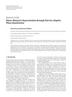
Figure 1 shows the employed rate function including the
Shannon reference with and without considering the LTE
overhead.
Note that the Shannon bounds inherently assume a per-
fect selection of modulation and coding schemes. However
in the uplink, due to fluctuating interference, this selection
can not be perfect by definition, even not in static channel
conditions. Furthermore imperfect channel estimation will
also degrade the performance. The consequence is a loss of
some dBs. On the other hand, the base stations typically
have 2 receive antennas, which is also not considered in
the Shannon bounds which will lead to a gain in the range
of 3 dB. Furthermore, frequency selective scheduling (e.g.,

though proportional fair scheduling) will lead to multi-user
diversity gain [18, 19].
In this work we will assume that those effects will
compensate each other such that the rate function used
here (red solid curve) is rather close to the Shannon
bound considering the overhead through cyclic prefix and
reference signals. Later on in Section 5.2 we will see that
this assumption leads to a good agreement with existing
simulation results.
3. Scheduling Probabilities
Let us now have a closer look at the scheduling probabilities
p
c
(v). We will consider several scheduler strategies. Note that
the random variable v
c
is discrete; it can adopt values v ∈ U
c
with the probability p
c
(v). For mathematical correctness, we
need to define a kind of idle value, for example, v
=−c,
with nonzero probability p
c
(−c) which represents the case
that no user is scheduled in cell c (at the considered time
and frequency, that is, a PRB is left empty). All other values
have the probability p
c

(v) = 0. With these definitions, we can
write (just for comprehension)
∞

v=−∞
p
c
(
v
)
= 1.
(11)
−10 −50 5 101520
0
2
00
40
0
600
800
1000
1200
Rate function
Shannon w/UL overhead
Pure Shannon bound
SINR (dB)
Throughput per PRB (kbps)
Figure 1: Rate function for the uplink.
3.1. Ge neral Expression. Let us define the average number of
PRBs

M
u
which is allocated to user u. Note that 0 ≤ M
u
≤
M
total
.GivenallM
u
’s in cell c, we can write the scheduling
probabilities as
p
c
(
v
)
=
⎧
⎪
⎪
⎪
⎪
⎪
⎪
⎪
⎪
⎪
⎪
⎨
⎪

⎪
⎪
⎪
⎪
⎪
⎪
⎪
⎪
⎪
⎩
M
v
M
total
for v ∈ U
c
,
1 −

u∈U
c
M
u
M
total
for v =−c,
0 for otherwise.
(12)
We observe that the scheduling probabilities depend
purely on the average number of assigned PRBs

M
u
’s. Hence,
we will investigate those elaborately in the following sections.
We will be looking at individual cells; we assume that cells in
general behave independently, that is, the random variables
v
c
’s are mutually independent, too.
3.2. Adaptive Transmission Bandwidth. The key difference
compared with the downlink is the fact that every user has
an individual power budget in the uplink. So we can shift
PRBs from one user to another, but not power. As a direct
consequence, the maximum number of PRBs which can be
given to a user without driving it into power limitation
depends on the difference between transmit power per PRB
P
(PRB)
T,u
(given by (2)) and the maximum transmit power P
max
which is typically called power headroom:
M
max,u
= floor
⎛
⎝
P
max
P

(PRB)
T,u
⎞
⎠
. (13)
EURASIP Journal on Wireless Communications and Networking 5
An uplink scheduler should never assign a user more
PRBs than this limit M
max,u
. Otherwise, looking at the
original power control equation (1), we observe that the
users would have to spread the same power over the assigned
PRBs instead of increasing the power with every assigned
PRB (the min operator in the PC equation (1) expires). This
results in an SINR loss which would eat up at least part of the
bandwidth gain. Furthermore, other (non-power-limited)
users can make much better use of the bandwidth. Finally,
spreading the maximum power over several PRBs would
increase the dynamic range problems. Note that for the PC
equation per PRB (2) we have already inherently assumed
that the scheduler does not exceed the aforementioned
limit. This behavior is typically called adaptive transmission
bandwidth [20].
Obviously this limits the maximum average number o f
PRBs as well, since every user can be scheduled at maximum in
everytimeslot,hencewehave
M
u
≤ M
max,u

.
(14)
3.3. Strict Resource Fair. The st raightfor ward definition of
the resource fair scheduler would be that the N
c
users in
cell c share the available resources, that is,
M
u
= M
total
/N
c
.
However, this may violate the power limitation of the UEs in
(14). If we require resource fairness, nevertheless, that is,
M
u
should be the same for all users, then every user can only get
as many PRBs as the worst user (using the highest transmit
power). We can write
M
u
= min

M
total
N
X(u)
,min

v∈U
X(u)
M
max,v

. (15)
An important observation is that this solution is also
throughput fair in the case of α
c
= 1 (with the exception
that power limited users would have smaller throughput).
Otherwise (α
c
< 1) close users get higher throughput since
the received power is higher and the interference is the same
for all users in a cell.
3.4. Modified Resource Fair. The previous scheduler has the
disadvantage that it may leave a lot of resources unused
although close users would still be able to extend their
bandwidth. Unfortunately, users at the cell edge with high
propagation loss cannot make use of the spare bandwidth
due to power limitation.
In another extreme solution we could try to always give
every user u its maximum allowed bandwidth M
max,u
. If this
does not exceed the available resources, that is,

u∈U
c

M
u
≤
M
total
, this is a viable approach. However, this will be
relatively unlikely in reality since already a single close user
could have enough transmit power to occupy more than
M
total
PRBs.
In this case we need to scale down the number of PRBs.
The simplest solution would scale down all M
max,u
’s in the
same way. However this would leave too much unfairness in
the system. Instead we prefer scaling down large M
max,u
’s and
bring this new solution as close as possible to the resource fair
case. We will call this solution modified resource fair although
it is in general not resource fair. However, in annex A we will
observe that this solution achieves the same fairness as the
typical resource fair definition in the downlink.
We propose a simple iterative method which starts
with the previous resource fair case. We define the indices
w
c,1
, w
c,2

, , w
c,N
c
such that they address all users u in cell
c in ascending order with respect to M
max,u
’s, that is, w
c,1
addresses the worst user in cell c, w
c,2
addresses the second
worst user, and so forth. We will formulate our algorithm as
follows:
(1) Initialize: i
= 1;

M = M
total
(2) Abbreviate u = w
c,i
(3) if

M/(

N − i +1)>M
max,u
(a) M
u
= M
max,u

(b)

M =

M − M
u
else
(c)
M
v
=

M/

N −i+1 for allv = w
c,i
, w
c,i+1
, , w
c,N
c
(d) exit
(4) Increment i
= i +1andgotostep2
In every iteration, we check whether the remaining
resource b udget

M equally shared among the remaining
N
− i + 1 exceeds the PRB limit M

max,u
of the worst of
the remaining users u. If yes, the worst remaining user
gets its maximum number of PRBs M
max,u
, and we assign
the remaining budget in the next iteration. Otherwise the
remaining budget is equal ly shared among the remaining
users, and we exit the algorithm.
Note again that in this solution the worst u ser gets the
least amount of resources, but the maximum it can afford.
With a high number of users this case will converge against
the previous “Resource Fair” case.
3.5. Throughput Fair. In this section we try to approximate
a throughput fair solution. We have already mentioned
that the number of PRBs is limited for the users. Since
the interference is the same for all users the throughput
achievable by all users is determined by the worst user (in
particular for α<1). The true throughput fair solution
employs the rate function and writes as
M
u1
M
u2
=
R
(
SINR
u2
)

R
(
SINR
u1
)
(16)
for two users u1andu2 in the same cell. Note that
throughput fairness is required per cell. Unfortunately the
SINRs are not known so far; recall that the M
u
’s are needed
to calculated scheduling probabilities and thereby the SINRs.
Thereforewewillgivetwodifferent approximations in the
following.
As a first approximation, we will do the simplifying
assumption that the throughput is proportional to the SINR,
that is, we assume linear rate function. From (7)weobserve
that the average SINR of a user within a certain cell is
proportional to the received power (since the interference is
6 EURASIP Journal on Wireless Communications and Networking
−2 0 2 4 6 8 10 12 14
0
0.5
1
1.5
2
2.5
3
3.5
4

4.5
5
Required number of PRBs
Reference user gets 3PRBs
Linear approximation
Log2 approximation
Real, SINR
=−6dB
Real, SINR
=−2dB
Real, SINR
= 4dB
Real, SINR
= 10 dB
Rx power relation P
R,u2
/ P
R,u1
(dB)
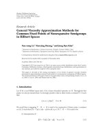
Figure 2: Approximation of required PRBs for throughput fair case.
cell specific). In this c ase the throughput fair criterion of the
previous equation degenerates to
M
u1
M
u2
=
SINR
u2
SINR

u1
=
P
R,u2
P
R,u1
.
(17)
Another approximation which is derived from Shannon’s
equation is
M
u1
M
u2
= log
2

1+
P
R,u2
P
R,u1

. (18)
The comparison of the two approximations is shown in
Figure 2 where we have used
M
u1
= 3. The true relation
obviously depends on the SINR range of the reference user

(cf. legend). The linear approximation fits for very small
SINR ranges; the log
2
approximation fits better for medium
SINR ranges.
Both approximations have the very nice property that
they only depend on the positions of the users within a cell
and not on intercell interference or other cells in general.
With those assumptions, we can formulate the throughput
fair (approximated) solution in three steps.
First we assume that the worst user gets the maximum
number of PRBs:
M
v
= M
max,v
v = arg
u
min
u∈U
c
M
max,u
.
(19)
Next we derive the number of PRBs for all the other users in
the cell by applying equation (17)
M
u
= M

v
·
P
R,v
P
R,u
, ∀u
/
= v
(20)
or (18)
M
u
= M
v
· log
2

1+
P
R,v
P
R,u

, ∀ u
/
= v. (21)
Finally we need to check whether we have exceeded the
resource limit. In this case, we have to scale down all
M

u
’s
by the same factor in order to fit into the available resources
whilst maintaining the throughput fairness:
M
u
= M
u
·
M
total
max

M
total
,

u∈U
c
M
u

.
(22)
3.6. Quality of Service. A drawback of the previous methods
is that we cannot define a target QoS or a user satisfaction
level. Inherently the methods were based on the best effort
and full buffer assumption. The users always have data to
transmit on one hand; on the other hand they do not have to
meet a certain target, that is, they are satisfied with whatever

resources
M
u
they get.
For a variety of services a certain QoS target has to be
met. For instance, users are only satisfied if they get a certain
bit rate D
u
. If they get less, they a re unsatisfied. On the other
hand, they typically cannot transmit more than D
u
, so the
system will assign only the resources
M
u
such that the target
rate is fulfil l ed, not more. Such a behavior is called constant
bit rate (CBR) service.
Initially, let us assume that the SINRs are already known.
We will resolve this assumption in the subsequent section.
The approach is very similar to the approach in [13]. In
order to achieve the target rate D
u
whilst observing the power
(and therefore resource) limitation in uplink, we write the
requiredaveragenumberofPRBsforuseru as
M
(req)
u
= min


M
max,u
,
D
u
R
(
SINR
u
)

,
(23)
where R(SINR
u
) is the rate function introduced in
Section 2.5. It is important to observe that a user cannot
be satisfied if the min operator expires, irrespective of the
traffic situation in the own cell (even if the user were alone).
The only way to improve those users is to decrease the
intercell interference, which requires modifications in the
neighboring cell such as decreasing the P0 [21]. Note that
any of those modifications is likely to reduce the QoS level in
the neighboring cell.
A cell can be defined in overload if the sum of
the required resources exceeds the available resources,

u|X(u)=c
M

(req)
u
>M
total
. In this case contention control
would drop some users (or, equivalently, admission control
would not even have admitted some users). We assume that
those control mechanisms work arbitrarily, that is, they do
not prefer some (e.g., close) users and discriminate others
(e.g., far users). This case can be modeled by applying the
same scaling procedure as in (22):
M
u
= M
(req)
u
·
M
total
max

M
total
,

u∈U
c
M
(req)
u


(24)
This scaling procedure would basically make every user
unsatisfied. However note that the scheduling probabilities
here are needed to calculate SINRs. Performance metrics w ill
be discussed in Section 4. Alternatively, we could make use of
admission control functionality here, which basically would
EURASIP Journal on Wireless Communications and Networking 7
select a subset U
sub,c
∈ u | X(u) = c (and drops the other
users) such that

u∈U
sub,c
M
(req)
u
>M
total
is fulfilled.
We would like to emphasize again that we have assumed
that the SINR
u
’sarealreadyknown.However,weactually
need the scheduling probabilities to calculate the SINR
u
’s
based on (7). So in contrast to the strict resource fair,
modified resource fair and (approximated) throughput fair

solutions of the previous sections, we unfortunately have not
found a closed form solution for the QoS case. This problem
is very similar to the downlink problem as described in [13].
3.7. Comparison with Real-World Schedulers. In the fol-
lowing we will discuss how real schedulers would map
to the previously introduced strategies. The most popular
scheduler is a proportional fair (PF) scheduler. The pure
PF strategy is resource fair [18, 19]. However, unfortunately
the PF definition in the uplink is not as straightforward
as it is in the downlink due to power control and power
limitation. Most of the uplink PF strategies in LTE will use
adaptive transmission bandwidth and will be very close to the
modified resource fair definition introduced in Section 3.4,
when assuming full buffer/best effort trafficmodels(i.e.,
no further QoS constraints), compare, for example, [20].
Note that the scheduling gain, that is, the fact that the SINR
conditioned on a user being scheduled gets better, goes into
the throughput mapping discussed in Section 2.5 and not
into the scheduling probabilities. Hence, PF and round robin
strategies are equivalent f rom the perspective of scheduling
probabilities (both are resource fair).
Furthermore, the PF strategies typically have to be
extendedwithQoSconstraintssuchasatargetbitrate,
minimum bit rate, or delay constraints. Those extended PF
versions will come closer to the QoS scheduler described
in Section 3.6. Once again, the reduced scheduling gain
(through more QoS constraints) is considered in the
throughput mapping, rather than in the scheduling proba-
bilities.
3.8. Initialization of the SINRs. In this section we will

propose 2 different solutions. Let us first recall the SINR
definition from (7)
SINR
u
= P
R,u
· Exp{···}.
(25)
The first observation is that the abbreviated expectation
Exp
{···} is only cell specific and not user specific. Hence,
for a first guess of the
M
u
’s according to (23)and(24), we
only need to approximate a single value rather than N
c
user-
specific SINR
u
’s, which seems to be a much simpler problem.
If we are applying the framework in this paper to a dynamic
simulator with a continuous time axis, we can simply take
the guess of the expectation from the previous time step.
Similarly, we can read that once we know the SINR
u0
of one
user u0 (e.g., the worst user), we know all the others by the
simple relation
SINR

u
= SINR
u0
·
P
R,u
P
R,u0
.
(26)
The advantage is that it might be easier to make a guess
on the SINR since it is a relative number rather than a guess
on the expectation which is an absolute number. In particular
the SINR of the worst user in a cell is rather likely to be very
small. So the second proposal is to set the SINR of the worst
user in every cell to a predefined value SINR
init
(e.g., 0 dB),
and the other user’s SINR in the same cell are derived from
that according to (26). This method has the advantage that it
also works with so-called snapshot-like simulators which do
not have a time axis. In a dynamic simulator, this approach is
probably less accurate than the first one.
4. Performance Metrics
So far, we have an (almost) analytical expression SINR
u
for
the average SINR of every user in an LTE uplink network.
Furthermore, we have already discussed the average number
M

u
of assigned PRBs for different scheduling strategies. Note
that in the QoS case the
M
u
’s actually depend on the SINRs
which are not known when calculating the
M
u
’s. Hence,
before calculating performance metrics we should update the
M
u
’s with the more accurate values of the SINRs.
From these SINR
u
’s and M
u
’s we now can star t deriving
several capacity metrics such as average cell throughput,
throughput percentiles, or number of (un)satisfied users.
4.1. Throughput Metrics. In the simplest case, we calculate
the user throughputs as
R
u
=
M
u
· R
(

SINR
u
)
.
(27)
From those rates we can calculate a total network through-
put, throughputs per cell, or throughput percentiles. In
principle we could also check whether users are satisfied by
comparing their data rates with the rate requirements D
u
’s.
However recall that in (24) we have scaled down the
M
u
’s of
all users in case of an overload. In this case, all users would
fall below their D
u
’s although in reality it might be sufficient
to drop very few users to make the rest satisfied again.
Furthermore, it would be interesting to have a quantitative
notion of how much overloaded a cell is and how many users
are unsatisfied in fact. So for the QoS case, we will define
more appropriate performance metric in the following.
4.2. Overload and Unsatisfied Users. Exactly as in [13]we
return to the required number of PRBs from (23)anddefine
a virtual cell load
ρ
c
=


u∈U
c
M
u
(req)
M
total
,
(28)
which can exceed 1 thereby indicating the degree of overload.
For instance,
ρ
c
= 1.1 means a 10% overloaded cell, and
ρ
c
= 2 means that the cell is double overloaded, that is,
half of the users will be unsatisfied. Again assuming that an
admission/contention control would exclude arbitrary users
(not preferably cell edge users), we can write the number of
unsatisfied users in cell c as
Z
load,c
= max

0, N
c
·


1 −
1
ρ
c

. (29)
8 EURASIP Journal on Wireless Communications and Networking
This number accounts for dissatisfaction through overload.
In addition, we will also have unsatisfied users through power
limitation as already discussed in the context of (23), even if
the virtual load is very small. We simply count their number
in cell
Z
power,c
=





u ∈ U
c
| M
max,u
<
D
u
R
(
SINR

u
)





, (30)
where
|A| returns the size of the set A. A further
limitation on cell level is given by the fact that the number
of users which can be scheduled at the same time is
constrained by the available resources for control channels
(physical downlink control channel PDCCH in LTE). Note
that this can be a painful restriction in particular in the
uplink, where the individual UE power budgets limit the
ability of following an aggressive TDMA strategy. With
our mathematical framework we can easily capture this
limitation as well. Assume that the maximum number of
schedulable users in cell c per TTI is given by K
tot,c
. (This is a
simplification. In LTE this is not a hard limit, but it depends
on the user positions.) The control channel consumption
is minimized by a scheduling strategy which would always
assign the maximum number of resources M
max,u
according
to (13) to a scheduled user. This maximized the number
of TTIs in which a user is not scheduled, that is, where it

does not require any control resources. Hence, the (averaged)
minimum number of required control channels required by
user u per TTI is
K
u
=
M
(req)
u
M
max,u
,
(31)
using the required number of PRBs
M
(req)
u
from (23). Note
that K
u
≤ 1. Obviously, the control channels will definitely
(even without any delay requirement) cause dissatisfaction
in case

u∈U
c
K
u
>K
tot,c

.
(32)
Equivalent to the load dissatisfaction we will again assume
that admission/contention control would exclude arbitrary
users and thus we can define the number of unsatisfied users
due to control channel limitation as
Z
ctrl,c
= max

0, N
c
·

1 −
K
tot,c

u∈U
c
K
u

. (33)
Finally we have to combine the three metrics Z
load,c
, Z
power,c
,
and Z

ctrl,c
to a single number of unsatisfied users per cell.
With our high level of abstraction this is quite challenging
since the sets of load-, power-, and control-unsatisfied
users might be overlapping. A heuristic approach would
exclude users one by one (power-limited users first) and
recalculate the metrics until dissatisfaction has disappeared.
Another approach exploits the intuitive fact that the set of
load- and control-limited users (i.e., the cell level metrics)
are obviously fully overlapping. The set of power-limited
users (user-level metric) will be rather disjoint. With those
assumptions we approximate the total number of unsatisfied
users in cell c as
Z
total,c
= max

Z
load,c
, Z
ctrl,c

+ Z
power,c
.
(34)
5. Results
A dynamic system level simulator has been implemented
based on the derivations in the previous chapters. In this sec-
tion we will present some results with standard assumptions

(such as full buffer traffic, proportional fair scheduler), and
we will show that those are very close to other simulation
results which have been agreed for by several companies in
[9, 22]. Furthermore, we will present results with CBR traffic,
and we will also look at an irregular network with SON
adaptation of the power control parameters. Finally we will
elaborate on the huge runtime performance.
5.1. Simulation Assumptions. We will use standard assump-
tions as proposed in [16], comprising a network of 19 LTE
base stations with an intersite distance of 500 m, serving
57 hexagonal cells (sectors). Pathloss law, shadowing model,
and horizontal beam pattern are also taken from [16], a
vertical pattern is not used. The users are moving with a
speed of 3 km/h, and they are handover to another cell if
the received signal strength (measured on downlink reference
signals) with respect to the new cell is 3 dB better than that
with respect to the serving cell (handover hysteresis). One
simulation step is 100 ms, that is, the network performance
is evaluated 10 times a second.
We are using homogeneous P0 values of P0
=−52 dBm
or P0
=−58dBm and a homogeneous α value of α =
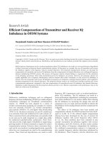
0.6. The resulting distribution of transmit power per PRB
is shown in Figure 3. Note that this distribution does not
depend on the scheduling mechanism or traffic model since
we record one power value for every user per simulation step.
It is obvious that the larger P0 setting of
−52 dBm leads
to higher transmit powers. In this case we can also identify

the maximum transmit power of 23 dBm.
5.2. Full Buffer Traffic. We will start with the simple assump-
tion of a full buffer traffic model and a modified resource fair
scheduler as presented in Section 3.4. Users are uniformly
dropped into the network area such that every cell serves an
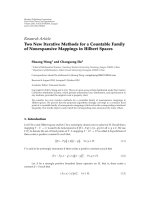
average of 10 users. The distribution of the user throughputs
according to (27)isgiveninFigure 4.
As expected we observe slightly higher user throughputs
with the larger P0 value. However, the differ ence between
the curves is smaller in the lower part of the plot, since the
power limitation is more critical with the smaller P0 value.
The 5% percentiles (which is typically referred to as cell edge
throughput) are 420 kbps and 503 kbps whereas the average
cell throughputs are 7.3 Mbps and 8.5 Mbps, respectively.
This is in very good agreement with the simulations in
[9, 22]. The results of different companies are compared in
[22] for the reference case which we have used as well. The
cell throughput results are in the range between 6.3 Mbps
and 1.01 Mbps, with an average of 8.6 Mbps (which is also
the result of [9]). The cell edge results span from 100 kbps to
EURASIP Journal on Wireless Communications and Networking 9
−15 −10 −50 5 10152025
0
0.1
0.2
0.3
0.4
0.5
0.6
0.7

0.8
0.9
1
Tx power (dBm)
P0 =−52 dBm
P0
=−58 dBm
Cumulative distribution function
Figure 3: Distribution of Tx Power per PRB.
0 200 400 600 800 1000 1200 1400
0
0.1
0.2
0.3
0.4
0.5
0.6
0.7
0.8
0.9
1
User throughput (kbps)
P0
=−52 dBm; average TP = 8.5 Mbps
P0
=−58 dBm; average TP = 7.3 Mbps
Cumulative distribution function
Figure 4: Distribution of user throughput in modified resource fair
case.
460 kbps with an average of 260 kbps. Obviously our results

are a bit too optimistic in terms of cell edge throughput
which could be a consequence of the neglected fast fading,
and, even more important, of handover gain, which is
included in our simulations with full mobility.
5.3. Constant Bit Rate Traffic. Next we will assume a constant
bit rate traffic model and a QoS scheduler as presented in
Section 3.6.Different target data rates are assumed, namely,
96 kbps, 256 kbps, and 512 kbps. Again, users are uniformly
dropped into the network; however, the average number of
users per cell is varied from 5 to 80. Let us first look at the
percentage of unsatisfied users due to power limitation Z
power
as given by expression (30)inFigure 5.
We observe the following behavior.
(i) All cur ves reach a maximum and then do not grow
any further. The reason is that the actual load is
limited and cannot exceed 100%. So the interference
will also not grow with the number of users, and the
SINRs will not decrease.
(ii) The (power) dissatisfaction level is larger for higher
data rates. This is quite obvious.
(iii) The (power) dissatisfaction level is larger for the
larger P0
=−52 dBm. With smaller P0, the users
can afford more PRBs, compare (14), whereas the
interference level goes down as well (note that the
other cells will reduce P0 as well in our model). So
the SINRs remain the same as long as we do not enter
noise limited regimes.
(iv) With 512 kbps and P0

=−52 we even have a
“dissatisfaction floor,” that is, there will be power
limited users even in an empty system. That is, high
uplink data rates can only be supported with small
P0 values (or by relaxing the ATB power constraint
(14)).
Note that the previous figure did not take into account
users which cannot be ser ved due to the lack of bandwidth.
Figure 6 shows the total number of unsatisfied users accord-
ing to (34), that is, the sum of power- and lo ad-unsatisfied
users. Control limitation is not considered, that is, K
total
c
=
∞
.
Certainly we can recognize the aforementioned dissatis-
faction floor for 512 kbps and P0
=−52 dBm in this figure.
Otherwise, the impact of the P0 value is almost negligible
since adding users beyond 100% virtual load obviously
means load-unsatisfied users hiding the aforementioned
limit for the dissatisfaction level due to the power constraint.
If we target a typical overall dissatisfaction level of 5%,
the uplink can satisfy 10, 21, and 56 user with 512 kbps,
256 kbps, and 96 kbps, respectively. The cell throughput w ith
the smaller rates is around 5.4 Mbps whereas the 512 kbps
case is slightly worse with 5.4 Mbps due to the more critical
power limitation.
As expected the CBR capacity is significantly below the

best effort capacity. However, the difference is smaller than
in the downlink, since the power control compensates for a
part of the SINR loss of cell edge users.
5.4. Heterogeneous Scenario. Next we will leave the homoge-
neous standard scenario and continue with a heterogeneous
scenario with different cell sizes and nonuniform user
concentrations. Figure 7 illustrated the scenario which has
been proposed in [23]. The eNBs are located on an irregular
grid, 8 users are dropped into every cell, and additional 42
users (i.e., 50 users in total) are dropped into cell no. 11
simulating a hot spot. All users use a CBR of 64 kbps. For
every cell c an individual P0
c
is chosen such that the min
operator in the power control equation (2) expires in roughly
5% of the cell area.
10 EURASIP Journal on Wireless Communications and Networking
0 1020304050607080
0
10
20
30
40
50
60
Number of users per cell
Power unsa
tisfied users (%)
P0 =−52 dBm, CBR = 96 kbps
P0

=−52 dBm, CBR = 256 kbps
P0
=−52 dBm, CBR = 512 kbps
P0
=−58 dBm, CBR = 96 kbps
P0
=−58 dBm, CBR = 256 kbps
P0
=−58 dBm, CBR = 512 kbps
Figure 5: Number of unsatisfied users due to power limitation.
0 1020304050607080
0
10
20
30
40
50
60
Number of users per cell
Total unsatisfied users (%)
P0 =−52 dBm, CBR = 96 kbps
P0
=−52 dBm, CBR = 256 kbps
P0
=−52 dBm, CBR = 512 kbps
P0 =−58 dBm, CBR = 96 kbps
P0
=−58 dBm, CBR = 256 kbps
P0
=−58 dBm, CBR = 512 kbps

Figure 6: Total number of unsatisfied users.
We will also look at load adaptive power control (LAPC)
as proposed in [24] where the P0
c

s are reduced in cells
which only carry a small load. In the CBR model reducing
P0
c
blows up the resource consumption since the resulting
SINR loss has to be compensated by bandwidth. We use a
very similar approach to [24] and update the P0
c
(t)attime
−3000 −2000 −1000 0 1000 2000
−2000
−1500
−1000
−500
0
500
1000
1500
2000
1
2
3
4
5
6

78
9
10
11
12
13
14
15
16
17
18
19
20
21
22
23
24
25
26
27
28
29
30
31
32
33
34
35
36
Distance (m)

Distance (m)
Figure 7: Cell layout.
step t depending on the previous value P0
c
(t − 1) and the
previous virtual load
ρ
c
(t − 1) (note that this equation is in
dB scale):
P0
c
(
t
)
= min

P0
c
, P0
c
(
t
− 1
)
+10log
10


ρ

c
(
t
− 1
)
ρ
target

,
(35)
where ρ
target
is the virtual load which we are targeting. In
theory we may want to target 100%; however, experience
has shown that a margin should be left for handover users
so that we w ill use ρ
target
= 80%. The rule means that we
increase the current P0
c
(t) if the load is above target, and we
decrease it if the load is below the target; however, we will not
increase the initial P0
c
which has been defined above. Note
that this automatic adaptation of a cell parameter can already
be considered as a SON mechanism.
Figure 8 depicts the virtual loads in the overloaded cell
no.11 and its neighbors over time where we have switched
on the LAPC at t

= 42 sec. Before that, the virtual loads are
rather small (except the overloaded cell no.11) and different
in every cell depending on the exact position of the users and
the cell shape/size. After switching on the LAPC the virtual
load in all low-loaded cells approaches the target ρ
target
=
80%.
The time characteristics of the corresponding P0
c
(t)s
are shown in Figure 9. Without LAPC we can observe that
the P0s depend on the cell size. Large cells have small P0s
and vice versa (due to the aforementioned 5% rule). After
switching on LAPC, the low-loaded cells reduce their P0s
whereascellno.11doesnotchangeit.
Now let us look at the impact of the LAPC on the
distribution of the interference over thermal (IoT) values.
Those are based on the S samples used for the Monte
Carlo approach defined in (10); the exact definition of the
(instantaneous) IoT is given by
IoT
c,s
=

i
/
= c
I
c,v

i,s
+ N
N
(36)
EURASIP Journal on Wireless Communications and Networking 11
0 20406080100
0
0.2
0.4
0.6
0.8
1
1.2
1.4
1.6
1.8
2
Virtual load
Cell #11
Cell #8
Cell #9
Cell #10
Cell #12
Cell #30
Cell #28
Time (s)
Figure 8: Virtual load in overloaded cells no.11 and neighbors.
leading to S · timesteps IoT samples per cell. Figure 10 shows
the cumulative distribution function of the IoT values (in
dB) in cell no.11 before and after switching on LAPC, and

it also displays the linear and the harmonic averages of the
IoT given by
IoT
lin,c
=
1
S
·
S

s=1
IoT
c,s
,
IoT
harm,c
=
⎛
⎝
1
S
·
S

s=1
1
IoT
c,s
⎞
⎠

−1
.
(37)
With LAPC the CDF is steeper since the users spread
their data rate over a larger bandwidth leaving less PRBs
unused (without interference) and leading to a smoother
interference. The interference of an individual user per PRB
certainly goes down significantly (with the P0reduction);
however, it has to occupy more PRBs to reach its CBR.
Still, the linear average of the IoT is smaller with LAPC
since the rate function is concave over a wide area meaning
that decreasing the power can be compensated by a smaller
increase of the bandwidth. However, the harmonic average
shows a surpr ising picture. The harmonic average decreases
with LAPC which is a consequence of the larger variance
of the IoT. Note that we have clearly shown in Section 2.3
that the harmonic average is actually the relevant measure.
This also manifests in the distribution of the average user
SINRs defined in (7) which are shown in Figure 11 for the
overloaded cells.
The LAPC has degraded the SINR in the overloaded cell
even though the P0 has not been reduced there since the
more fluctuating interference obviously offers more potential
for the link adaptation (which is assumed to be ideal in
our model). This is also visible in the virtual load of the
0 20406080100
−66
−64
−62
−60

−58
−56
−54
−52
−50
−48
Cell #11
Cell #8
Cell #9
Cell #10
Cell #12
Cell #30
Cell #28
Time (s)
P0 (dBm)
Figure 9:P0settingsinoverloadedcellno.11andneighbors.
024681012141618
0
0.1
0.2
0.3
0.4
0.5
0.6
0.7
0.8
0.9
1
Without LAPC
With LAPC

Linear average w/o LAPC
Harmonic average w/o LAPC
IoT samples (dB)
Linear average w/ LAPC
Harmonic average w/ LAPC
Cumulative distribution function
Figure 10: IoT distribution in overloaded cell no.11 with and
without LAPC.
overloaded cell no.11 in Figure 8 which has slightly been
increased by LAPC (as a result of the decreased SINRs). This
is a contrast to the results in [24] where LAPC helps to
improve the system. Fluctuating interference has a negative
impact on link adaptation (i.e., selection of modulation
and coding schemes, scheduling, etc.). In other words,
smoothening the interference through LAPC will improve
link adaptation. Unfor tunately this effect is not covered
12 EURASIP Journal on Wireless Communications and Networking
−202468101214161820
0
0.1
0.2
0.3
0.4
0.5
0.6
0.7
0.8
0.9
1
Without LAPC

With LAPC
Average SINRs (dB)
Cumulative distribution function
Figure 11: SINR distribution in overloaded cell no.11 with and
without LAPC.
in our simplified model, where link adaptation is always
assumed to be ideal. Hence, our model can exploit the
aforementioned potential offered by fluctuating interference,
which is not the case in realit y.
Although we have gained important insights by this
analysis, it also reveals a current limitation of the model.
A remedy could be based on the principles of [25],
where the rate function is elaborated by the introduction
of a correlation between the SINR at the moment of
choosing the modulation and coding scheme and the
moment of applying it (where the interference might
have changed). This correlation would increase through
LAPC.
5.5. Simulation Runtime. Finally we will look at the run-
time performance of the simulation. Figure 12 shows the
simulation time for one simulation step versus the average
number of users per cell. It turned out that the number
of samples used for the Monte Carlo integration in (10)
has significant impact. As already mentioned, convergence
is achieved for S>1000. Fortunately we observe that
further reduction of this number does not bring additional
runtime benefit. The increase is linear with respect to the
number of users, which is not surprising. With 50 users per
cell and a simulation step of 1 sec, which is sufficient for
many applications, we are a factor 2 above real-time. Recall

that we have a fully heterogeneous 57-cell network, and no
homogeneous properties are exploited.
6. Conclusions
We have presented a very efficient modeling approach for
uplink investigations focussing on the LTE standard. QoS
and radio resource management (which typically work on a
millisecond time scale) are modeled in a very abstract but still
10 20 30 40 50 60 70 80 90 100
0
0.5
1
1.5
2
2.5
3
3.5
4
Average number users per cell
Runtimefor1simulationstep
500 IoT samples
1000 IoT samples
5000 IoT samples
10000 IoT samples
Figure 12: Runtime in a 57-cell environment on a 2.4 GHz CPU.
accurate way such that the essential behavior is still included.
By those means we can decrease simulation runtime far
below real-time.
This is in particular helpful, even necessary, for simu-
lations covering long time intervals. The most important
applications are investigations on self-optimizing networks

since SON mechanisms are typically very slow control loops
and converge over hours or even days. Conventional system
level simulators cannot serve this purpose. On the other
hand, QoS and mobility issues are of utmost importance
and can not be neglected when studying SON which makes
static tools inappropriate as well. We are closing the gap
between too slow but elaborate system level simulators with
full mobility and QoS support on one side and rough static
simulators which can lead to very fast results.
We have seen that uplink modeling is much more com-
plicated than downlink modeling. The key differences are
the uplink power control (including the associated individual
UE power budgets) and the multiple-access structure of the
uplink (leading to extremely fluctuating interference). We
have derived an average uplink SINR which is equivalent to
the downlink SINR which is typically intuitively used. We
have observed that the uplink interference has to be averaged
in a har monic way.
Different traffic/scheduler assumptions have been dis-
cussed. Again in contrast to downlink, there is no unique
definition of a resource fair scheduler in the full buffer
case. We have given two solutions called strict and modified
resource fair. Furthermore, throughput fair solutions as
well as CBR solutions targeting a given bit rate have been
defined. In order to evaluate the system performance we have
discussed uplink satisfaction in the CBR case. In addition
to load limitation, we have observed that satisfaction due
to power limitation and due to control channel limitation is
highly relevant in uplink, too.
EURASIP Journal on Wireless Communications and Networking 13

Limitations of the abstract models have been addressed as
well. In particular, RRM details such as the exact algorithms
for MCS selection, multi-user diversity gains, and imperfect
channel estimation are hidden behind the abstract models
(although the essence of fairness issues is considered).
Furthermore, the capability to consider more elaborate
trafficmodels(different from pure CBR and pure best effort)
is limited. We are giving an outlook on possible extensions in
Appendix B.
We have given simulation results using the derived
modeling approach. In the specified LTE test cases our results
match very well the typical performance assumptions. We
have also given results for the CBR case using different
target bit rates and analyzed the impact of power limitation.
Finally we were looking at a heterogeneous scenario with
different cell sizes and non-uniform user placement. We
have considered load-adaptive power control as an example
for a SON mechanism. This scenario has revealed some
limitations of our modeling approach which have to be
improved in the future.
In this paper we have only looked at a small subset of
the proposed SON use cases since the focus was on the
introduction of the framework. Certainly the model can
be used for all other SON use cases as well, such as load
balancing, coverage and capacity optimization, or mobility
robustness optimization.
Appendices
A. Discussion of Uplink Fair ness
In this section we will compare the uplink fairness with the
downlink fairness. We will show that the modified resource

fair scheduler in the uplink achieves a comparable f airness as
a typical resource fair scheduler in downlink.
In downlink, the SINRs on a PRB degrade towards
the cell edge more severe than the pathloss law, since
the interference grows in addition. With a resource fair
scheduler, the throughputs behave accordingly. However, we
can improve cell edge users arbitrarily by assigning them
more PRBs (nonresource fair scheduling).
In the uplink, the degradation towards the cell edge is
different. By purely looking at the power control equation
(2), bandwidth limitation (13), and SINR definition (7), we
make the following observations.
(1) The uplink interference is induced at the eNB
antennas and therefore is the same for all users
(as long as we do not assume intercell interference
coordination).
(2) Assuming no power control α
= 0 (resulting in
strict resource fairness, that is, one PRB per user),
that is, each UE transmits w ith maximum power,
the SINRs per PRB would degrade with the pathloss.
Note that this is still “fairer” as in the downlink
(where interference increases in addition).
(3) Assuming power control with ful l pathloss compen-
sation α
= 1 (and adaptive transmission bandwidth),
that is, all UEs are received with the same power
per PRB, the SINRs per PRB would be the same for
all UEs, but the assigned bandwidth degrades with
the pathloss, copmared with (14) unless the P0s are

rather small. So the throughputs degrade with the
pathloss (which is a little steeper than the upper case
due to concavity of the rate function).
(4) Assuming power control with fractional pathloss
compensation 0 <α<1 (and adaptive transmission
bandwidth), the SINRs per PRB would degrade less
severely than the pathloss; however, the assigned
bandwidth degrades with the “rest” of the pathloss
law. So in total the throughputs again will degrade
with pathloss, with the slope being in between the
upper two cases.
So in either case the throughputs will degrade with the
pathloss, either via SINR deg radation (for α<1) and / or
via the ATB scheduler. The degradation will be similar to the
downlink. All cases refer to the definition of the modified
resource fair scheduler. Thestrictresourcefair solution will
lead to more fairness, that is, less throughput degradation for
α>0. For the special case of α
= 1 strict resource fairness
even leads to throughput fair ness.
Despite similar fairness behavior, the uplink scheduler
has much less degrees of freedom to trade throughput among
the users (due to individual power budgets). The only way
to extend the strict throughput limit of cell edge users is
to reduce the intercell interference which unfortunately lies
outside the responsibility of the serving cell. Even more
severe, the neighbors can only decrease interference by
degrading their own users. Hence, whereas in downlink we
can trade throughputs between users, in uplink we need to
trade throughputs between cells.

B. Traffic Assumptions
We have already observed that the individual power limita-
tion in the uplink results in a bandwidth limitation M
max,u
(the number of PRBs for edge users is limited) and thereby
in a tight data rate limit. This is different from the downlink,
where basically each PRB comes along with its own power
budget, so that assigning more PRBs automatically means
assigning more power.
As a consequence, in the uplink we can only guarantee
small data rates to cell edge users. So if we want to assume a
common CBR model for all users, it has to be very small such
that the edge users have a fair chance to achieve it. With such
a setting there are basically 3 different methods how capacity
limit could be achieved.
(1) Common CBR. The straightforward solution is to con-
sider a large number of users. This would increase simulation
runtime, and large data rates would not occur at all.
(2) Common CBR Exte nded with Full Buffer. With a smaller
number of users we could think about distributing the excess
capacity (i.e., PRBs) among those users who stil l can afford
more PRBs. Basically this would be a mixture of CBR and full
14 EURASIP Journal on Wireless Communications and Networking
buffer model, which can be referred to as guaranteed bit rate
(GBR) model. The drawback is that we would need another
metric (in addition to the satisfied users due to load and
power) accounting for users with higher throughput (i.e.,
95% percentile). Furthermore we have to set a rule how the
excess capacity is distributed among the users.
(3) User-Specific CBR. Finally, we could set different bit

rate requirements D
u
for the users, for example, depending
on the pathloss. Edge users would get small D
u
’s, and
close users would get higher D
u
’s. This might be the most
convenient solution and probably the most realistic one as
well.However,weneedtofindanappropriateruletoset
the individual rate requirements D
u
’s, which is absolutely not
straightforward. We will propose a simple mechanism with
the following characteristics.
(a) We define a minimum data rate D
min
which lower-
bounds all rate requirements, that is, D
u
≥ D
min
.
(b) The rate requirement for the worst user v
c
(i.e., with
largest pathloss) in every cell c is set to the minimum
rate, that is,
D

v
c
= D
min
with v
c
= arg
u
min
u∈U
c
L
c

−→
q , Θ
c

. (B.1)
(c) The rate requirements for the other users are upscaled
according to the pathloss relation to the worst user v
c
D
u
= D
min
·

L
X(u)

(
−→
q
v
c
, Θ
X(u)
)
L
X(u)
(
−→
q
u
, Θ
X(u)
)

1−β
.
(B.2)
The fairness parameter β can be considered as “slope”
of the rate requirements. β
= 1obviouslymeansno
slope, that is, the same rate D
min
for all users which
converges to the common CBR solution. There is an
interesting relation to the power control parameter
α; setting β

= α will lead approximately to a
resource fair behavior, since the rate increase would
roughly be compensated by the increase in received
power through fractional power control; this would
be exactly true for a linear relation between SINR and
throughput and if we neglect the power limitation.
β
= 0 is the most aggressive setting which makes it
approximately equally tough for every user to achieve
its target.
For this special case of user-specific CBR setting, we will
now propose a special initialization for the SINRs. Recall that
the SINRs depend on the average number of PRBs
M
u
(or
scheduling probabilities, resp.); however, the performance
metrics depend on the SINRs in turn. For 3 ar tificial cases
we have proposed simple ways to calculate the
M
u
’s without
needing the SINRs in Sections 3.3, 3.4,and3.5.Theproposal
is a slight modification of the idea for the TP-fair case in
Section 3.5.Ineverycellc we start with an initial guess G for
the worst user’s
M
v
c
= G. From this guess we approximate

the resource consumption of
M
u
= G ·

L
X(u)
(
−→
q
v
c
, Θ
X(u)
)
L
X(u)
(
−→
q
u
, Θ
X(u)
)

α−β
(B.3)
if we neglect power limited users. As discussed before we
observe
(i) the resource fair behavior M

u
= G for α = β,
(ii) smaller resource consumption M
u
<Gfor close users
towards the throughput fair solution α
≤ β ≤ 1,
(iii) larger resource consumption M
u
>Gfor close users
towards the aggressive solutions 0
≤ β ≤ α;with this
setting, we can initialize the SINR calculation for the
user-specific CBR case depending only on a single
parameter G.
(4) Summary. We will now summarize the required hooks
for the traffic configuration with user-specific CBRs.
(i) The first is a m inimum rate requirement D
min
.We
propose values between 64kbps and 96kbps. Higher
valueswillalreadybecomecriticalforcelledgeusers.
(ii) The second is a slope β for the rate requirements.
β
= 1 means throughput fair behavior; smaller
values increase the rate requirements for closer users
depending on their pathloss relation to the worst
user, thereby forcing more load in the system. We
propose a setting between 0 and α.
(iii) The third is a guess G for SINR initialization. A first

proposal is G
= 1; however, this requires further
study.
References
[1] SOCRATES, “Self-optimisation and self-configuration in
wireless networks,” European Research Project, http://www
.fp7-socrates.org.
[2] M. D
¨
ottling and I. Viering, “Challenges in mobile network
operation: towards self-optimizing networks,” in Proceedings
of IEEE International Conference on Acoustics, Speech and
Signal Processing (ICASSP ’09), pp. 3609–3612, Taipei, Taiwan,
April 2009.
[3] M. Amirijoo, R. Litjens, K. Spaey et al., “Use cases, require-
ments and assessment criteria for future self-organising radio
access networks,” in Proceedings of the 3rd International
Workshop on Self-Organizing Systems (IWSOS ’08), pp. 275–
280, December 2008.
[4] “Next Generation Mobile Networks, Use Cases related to
Self Organising Network,” Overall Description, http://www
.ngmn.org/.
[5] 3GPP, “Self-configuring and self-optimizing network use cases
and solutions,” Tech. Rep. TR 36.902, />[6] U. T
¨
urke and M. Koonert, “Advanced site configuration
techniques for automatic UMTS radio network design,” in
Proceedings of the 61st IEEE Vehicular Technology Conference,
vol. 3, pp. 1960–1964, Stockholm, Sweden, May-June 2005.
[7]A.Lobinger,S.Stefanski,T.Jansen,andI.Balan,“Load

balancing in downlink LTE self-optimizing networks,” in
Proceedings of the 71st IEEE Vehicular Technology Conference,
Taipei, Taiwan, May 2010.
[8] K. Brueninghaus, D. Ast
´
elyt, T. Salzer et al., “Link performance
models for system level simulations of broadband radio
access systems,” in Proceedings of the 16th IEEE International
EURASIP Journal on Wireless Communications and Networking 15
Symposium on Personal, Indoor and Mobile Radio Communi-
cations (PIMRC ’05), vol. 4, pp. 2306–2311, Berlin, Germany,
September 2005.
[9] M. Rinne, M. Kuusela, E. Tuomaala et al., “A performance
summary of the evolved 3G (E-UTRA) for voice over internet
and best effort traffic,” IEEE Transactions on Vehicular Technol-
ogy, vol. 58, no. 7, pp. 3661–3673, 2009.
[10] A. Simonsson and A. Furusk
¨
ar, “Uplink power control in
LTE—overview and performance,” in Proceedings of the 68th
IEEE Vehicular Technolog y Conference (VTC ’08),Calgary,
Canada, September 2008.
[11] K. Majewski and M. Koonert, “Conservative cell load approx-
imation for radio networks with shannon channels and its
application to LTE network planning,” in Proceedings of the
6th Advanced International Conference on Telecommunications,
Barcelona, Spain, May 2010.
[12] 3GPP, “Simulation assumptions and parameters for FDD
HeNB RF requirements,” TDoc R4-092042, RAN WG4 Meet-
ing #51, San Francisco, Calif, USA, May 2009, http://www

.3gpp.org/.
[13]I.Viering,M.D
¨
ottling, and A. Lobinger, “A mathematical
perspective of self-optimizing wireless networks,” in Proceed-
ings of IEEE International Conference on Communications
(ICC ’09), Dresden, Germany, June 2009.
[14] 3GPP, “Stage 2 Description,” Technical Specification TS
36.300, />[15] 3GPP, “Physical layer procedures,” Technical Specification TS
36.213, />[16] 3GPP, “Physical layer aspects for evolved Universal Ter-
restrial Radio Access (UTRA),” Tech. Rep. TR 25.814,
/>[17] B. Zerlin, M. Ivrla
ˇ
c, W. Utschick, J. Nossek, I. Viering, and A.
Klein, “Joint optimization of radio parameters in HSDPA,” in
Proceedings of the 61st IEEE Vehicular Technology Conference
(VTC ’05), vol. 1, pp. 295–299, Stockholm, Sweden, May 2005.
[18] D. Tse and P. Viswanath, Fundamentals of Wireless Commu-
nications, Cambridge University Press, Cambridge, UK, 1st
edition, 2005.
[19] P. Viswanath, D. N. C. Tse, and R. Laroia, “Opportunistic
beamforming using dumb antennas,” IEEE Transactions on
Information Theory, vol. 48, no. 6, pp. 1277–1294, 2002.
[20] F. D. Calabrese, C. Rosa, M. Anas, P. H. Michaelsen, K.
I. Pedersen, and P. E. Mogensen, “Adaptive transmission
bandwidth based packet scheduling for LTE uplink,” in
Proceedings of the 68th IEEE Vehicular Technology Conference
(VTC ’08), Calgary, Canada, September 2008.
[21] M. Boussif, N. Quintero, F. D. Calabrese, C. Rosa, and J.
Wigard, “Interference based power control performance In

LTE Uplink,” in Proceedings of IEEE International Symposium
on Wireless Communication Systems (ISWCS ’08), pp. 698–702,
Reykjavik, Iceland, October 2008.
[22] “Next Generation Mobile Networks, Radio Performance Eval-
uation,” available at, />[23] J. Turkka and A. Lobinger, “Non-regular layout for cellular
network system simulations,” in Proceedings of the Inter-
national Symposium on Personal, Indoor and Mobile Radio
Communications (PIMRC ’10),Istanbul,Turkey,September
2010.
[24] M. Boussif, C. Rosa, and J. Wigard, “Load adaptive power
control in LTE uplink,” in European Wireless, Lucca, Italy, April
2010.
[25] M. Casta
˜
neda, M. T. Ivrla
ˇ
c, J. A. Nossek, I. Viering, and A.
Klein, “Outdated uplink adaptation due to changes in the
scheduling decisions in interfering cells,” in Proceedings of
IEEE International Conference on Communications (ICC ’08),
pp. 4948–4952, Beijing, China, May 2008.