Báo cáo hóa học: " Research Article Modeling On-Body DTN Packet Routing Delay in the Presence of Postural Disconnections" ppt

Hindawi Publishing Corporation
EURASIP Journal on Wireless Communications and Networking
Volume 2011, Article ID 280324, 19 pages
doi:10.1155/2011/280324
Research Article
Modeling On-Body DTN Packet Routing Delay in the Presence of
Postural Disconnections
Muhannad Quwaider,
1
Mahmoud Taghizadeh,
2
and Subir Biswas
2
1
Department of Computer Engineering, Jordan University of Science and Technology, Irbid, Jordan 22110-3030, Jordan
2
Department of Electrical and Computer Engineering, Michigan State University, East Lansing, MI 48824-1226, USA
Correspondence should be addressed to Subir Biswas,
Received 25 April 2010; Revised 19 August 2010; Accepted 17 September 2010
Academic Editor: Sergio Palazzo
Copyright © 2011 Muhannad Quwaider et al. This is an open access article distributed under the Creative Commons Attribution
License, which permits unrestricted use, distribution, and reproduction in any medium, provided the original work is properly
cited.
This paper presents a stochastic modeling framework for store-and-forward packet routing in Wireless Body Area Networks
(WBAN) with postural partitioning. A prototype WBANs has been constructed for experimentally characterizing and capturing
on-body topology disconnections in the presence of ultrashort range radio links, unpredictable RF attenuation, and human
postural mobility. Delay modeling techniques for evaluating single-copy on-body DTN routing protocols are then developed.
End-to-end routing delay for a series of protocols including opportunistic, randomized, and two other mechanisms that capture
multiscale topological localities in human postural movements have been evaluated. Performance of the analyzed protocols are
then evaluated experimentally and via simulation to compare with the results obtained from the developed model. Finally, a
mechanism for evaluating the topological importance of individual on-body sensor nodes is developed. It is shown that such

information can be used for selectively reducing the on-body sensor-count without substantially sacrificing the packet delivery
delay.
1. Introduction
1.1. Body Area Networks. A number of tiny wireless sensors,
strategically placed or implanted on a patient’s body, can
create a Wireless Body Area Network (WBAN)[1, 2]. A
WBAN can monitor vital signs, providing real-time feedback
for enabling many patient diagnostics procedures via contin-
uous monitoring of chronic conditions, or recovery progress
from an illness or surgical procedure. Data transaction
across such sensors can be point-to-point or multipoint-to-
point. While distributed detection of an athlete’s posture
[3, 4] would require point-to-point packet exchange across
various on-body sensors, applications such as monitoring
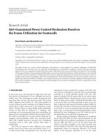
vital signs, as shown in Figure 1, will require all body-
mounted and/or implanted sensors [2, 5]toroutedata
multipoint-to-point to a sink node, which in turn can process
and relay the information wirelessly to an out-of-body
server. Data transaction can be also real-time or nonreal-
time. While patient monitoring type of applications would
require real-time packet routing, monitoring an athlete’s
physiological data can be collected offline for postprocessing
and analysis purposes. The routing protocols modeled in
this paper cater to this nonreal-time class of on-body
applications.
1.2. Short RF Range. Inthispaperwemodelon-body
packet routing mechanisms in the presence of topological
partitioning caused due to ultra-short wireless transmission
range and postural body movements. Short transmission
range is a common constraint for low-power RF transceivers

designed for embedded applications with limited energy
[6, 7], often supplied by harvested operations [8]. Such
situations are particularly pertinent for implantable body
sensors. Examples of ultralow range transceivers in the
literature include [9] with 0-1 m, [8] with 0.2–1 m, [10]
with 0.2 m, and [11] with 0-1 m transmission ranges. The
corresponding transmission powers vary between 0.75 mW
to 6 mW, which are within a range that can be handled
with common harvesting techniques such as piezoelectric
generation from body movements. Information available
in the literature on such low power RF transceivers is
summarized in Ta bl e 1.
2 EURASIP Journal on Wireless Communications and Networking
Sink
Source
Out-of-body
Server
Modalities:
- Blood pressure
-Heart rate
-Breathing rate
- Diabetes
-Temperature
-Humidity
-ECG
-Movement
-Proximity
-Direction
2
3

1
4 5
6
7
2
3
1
4 5
6
7
Figure 1: Body area sensor network.
Table 1: Low power and short range RF transceivers.
Reference
Tx Range
(meter)
Tx. Power
consumption
(mWatt)
Rx. Power
consumption
(mWatt)
[8]
0.2–1 1.5–3.5
∼2.5
[9]
0-1 2 2
[10]
0.2 0.75–3.75 0.75–3.75
[11]
0-1 6 5.1

1.3. Routing with Network Partitioning. Low RF ranges also
meanthatposturalbodymovementscangiverisetofrequent
partitioning or disconnection in WBAN topologies, resulting
in a body area Delay Tolerant Network (DTN) [12–17].
Such topological partitioning can often get aggravated by the
unpredictable RF attenuation caused due to signal blockage
by clothing material and body segments. Although real-time
applications such as patient monitoring may not be sup-
ported in the presence of topological partitioning, nonreal-
time applications such as athlete’s physiology monitoring
can still be supported using on-body DTN packet routing
across disconnected partitions. Performance goals for such
protocols will be to obtain (1) low end-to-end delay, (2) low
packet loss, and (3) low transmission energy consumption.
1.4. Novelty and Contribut ions. Thegoalofthispaperis
to develop analytical modeling mechanisms for computing
packet transfer delay for a series of DTN routing algorithms
that can be implemented in an on-body setting. Although
a number of papers in the literature [12–17] have studied
DTN routing in general settings, to our knowledge, this is
the first study that formally evaluates DTN routing delay
in a WBAN through analytical model development. The
dominating delay in DTN routing is contributed by packet
buffering caused due to topological disconnections. In the
absence of network congestions in low data-rate WBANs,
such buffering delays are usually much larger compared to
the congestion delay. That is why the congestion delay is
not modeled in this paper. Specific contributions of the
paper are as follows. First, we develop a prototype body
area network for motivating the on-body packet routing

problem and conducting on-body routing experiments with
the DTN routing protocols that are modeled and evaluated
in this paper. Second, a topology trace collection mechanism
is developed for wirelessly extracting network topology, as
a function of human postural dynamics, from the on-body
sensors to an off-body server. Third, analytical techniques
are developed for modeling the end-to-end packet delay for
a range of DTN routing algorithms, namely, opportunistic
[18–20] utility based [18, 20, 21], random [18, 20, 22],
PRMPL [23, 24], and DVRPLC [23, 24]. Fourth, the DTN
routing delays obtained from the developed model are
compared with results from on-body experiments from
the prototype WBAN and off-body simulation carried out
on network topology traces obtained from the prototype
WBAN. Finally, using the model and the topology trace data,
a detailed analysis is carried out for identifying noncritical
nodes in order to design a minimal WBAN topology from the
routing stand point. The novelty of this approach includes
(1) experimental evaluation of the proposed framework in a
practical prototype WBAN system and (2) development of
detailed delay models that can be useful for predeployment
system dimensioning, planning, and what-if analysis of real
body area networks.
2. Related Work
Most of the existing WBAN systems [1, 25–27] adopt star or
tree topologies on a connected graph, leading to end-to-end
EURASIP Journal on Wireless Communications and Networking 3
physical connectivity between any pair of on-body sensors
at any given point in time. However, these models do not
apply for the targeted DTN routing paradigm, which handles

topology partitioning leading to scenarios in which end-
to-end physical connectivity between node pairs may not
be present all the time. Such partitioning is caused mainly
due to the ultra short range RF transceivers as reported in
Section 1.2.
The existing research on routing in Delay Tolerant
Networks or DTNs is categorized [12, 13] as (1) replication
based (multiple copy) [14, 17, 18] and (2) single copy
[15, 19–21, 28]. The replication approach explores the ways
in which several copies of a packet can be disseminated
among several carrier mobile nodes to increase the chance
of delivery to the desired destinations. Most of routing
schemes proposed for DTN routing protocols belong to
this category [17, 29–31]. While providing good delay
performance, the primary limitation of these protocols
is their energy and capacity overheads due to excessive
packet transmissions. Further, under high traffic loads they
may suffer from severe contention and subsequent packet
drops that can degrade their performance and scalability
[12, 13, 31, 32]. For ultraresource-constrained WBANs,
such overheads are usually not acceptable. The single copy
forwarding mechanisms make use of information about the
connectivity and topology dynamics to make low-latency
forwarding decisions with minimal replication overhead.
The general principle is that when a node with a buffered
packet encounters another node, the packet is forwarded to
the encountered node only if it is more likely (than the node
currently buffering the packet) to visit the destination node.
For the above mechanisms to work as anything beyond
epidemic/viral routing [33], the nodes need to have certain

degree of spatial and temporal locality in their mobility and
meeting patterns. A notable DTN routing scheme in the lit-
erature is PROPHET [17] which is an extension of epidemic
routing [29]. PROPHET develops a probabilistic framework
for capturing the spatiotemporal locality present in the node
mobility pattern within a dynamically partitioned wireless
network. PROPHET can be implemented either in single
copy or in multicope mode. Node interaction localities can
be also captured in the form a per-link utility as detailed in
[18, 19]. The link utility can be formulated as its age [19–21],
formation frequency [19], and other historical parameters
that can effectively capture the nodes’ interaction localities.
Two additional routing protocols, namely, opportunistic
[18–20]andrandomized [19, 20], are also analyzed in the
literature for applications in which either there is no node-
interaction locality or such localities cannot be evaluated.
With opportunistic routing, a source node directly delivers
its packets to the destination node and buffers them till the
link with the destination is formed. In randomized routing,
packets are randomly routed following the hot-potato logic
[20]. Both these protocols are hugely outperformed by the
locality-based protocols [19, 20] due to their knowledge
about the properties of the links.
In the existing literature, the above mechanisms are all
applied to networks spanning across local to wide areas,
few extending all the way up to the interplanetary scale
[34], whereas in this paper the objective is to develop DTN
routing for WBANs with ultra short transmission range.
Also, the treated node mobility patterns in the literature are
generally very different from what is observed for on-body

DTN networks. The key objective of this work is to model
the delivery delay of a number of representative DTN routing
protocols, as identified above, in WBAN settings.
In [18, 19] the delay performance of single- and multi-
copy DTN routing is evaluated in the presence of random-
walk mobility without any specific locality information. The
analyzed utility in those papers was computed by capturing
short-term locality in nodes connectivity in the presence of
node location information. In this paper, however, a key goal
is to formulate modeling mechanisms that can capture multi-
scale topological localities in human postural movements
and use such locality information for modeling packet
routing delay. In addition to general purpose DTN routing,
including opportunistic [18–20], utility based [19–21], and
random [19, 20], two other protocols, namely, PRMPL [23,
35], and DVRPLC [23, 35], which are specifically designed
for on-body DTN routing, are also modeled in this paper.
3. Experimental Characterization of on-Body
Network Topology
To m o d el di fferent routing protocols we have implemented a
working WBAN prototype system. This section describes the
WBAN prototype and its application for experimental topol-
ogy characterization with varying body postural positions.
3.1. WBAN Prototype. A Wireless Body Area Network
(WBAN) is constructed by mounting seven sensor nodes
(attached on two upper-arms, two thighs, two ankles, and
one in the waist area) as shown in Figure 1.Eachwearable
node consists of a 900 MHz Mica2Dot MOTE (running
TinyOS operating system), with Chipcon’s SmartRF CC1000
radio chip ( and the sensor card

MTS510 from Crossbow Inc. ( The
Mica2Dot nodes run from a 570 mAH button cell with a total
sensor weight of approximately 10 grams. The default CSMA
MAC protocol is used with a data rate of 19.2 kbps.
Via software adjustments of the CC1000’s transmission
power, the transmission range is set to be in between 0.3 m–
0.6 m. By doing so, we are able to emulate the ultralow
transmission range for the embedded transceivers [8–11]
as reported in the literature. Note that the variation of the
range is caused due to the variability in antenna orientation,
clothing, and other on-body RF attenuation characteristics.
The sensors form a mesh topology with one or multiple
simultaneous network partitions. The topology and the
number of partitions change dynamically based on the
postural positions of the subject individuals. All experiments
in this paper correspond to multipoint-to-point routing in
which data from all other nodes are sent to node-6 (see
Figure 1), which is designated as the on-body sink node. This
node collects raw data and sends processed results or events
to an out-of-body server using a wireless link. This external
4 EURASIP Journal on Wireless Communications and Networking
SIT REC DWN STD WLK RUN
SIT REC DWN STD WLK RUN
SIT REC DWN STD
WLK
RUN
On
Off
Link:1–3
Link status

0 20 40 60 80 100 120
Time (s)
On
Off
Link:4–6
Link status
0 20 40 60 80 100 120
Time (s)
On
Off
Link:5–3
Link status
0 20 40 60 80 100 120
Time (s)
Figure 2: Variation of instantaneous link connectivity with postural mobility.
link is created between the on-body sink node and to an
out-of-body Mica2Dot radio node connected to a Windows
PC through a custom-built serial interface, running RS232
protocol.
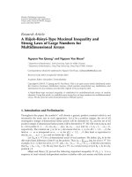
3.2. Var iations of Topology and Network Partitions. Exper-
iments were carried out for observing the impacts of
postural mobility on network partitioning. A human subject,
fitted with seven sensors, was asked to follow a predeter-
mined sequence of postures (SIT, SIT-RECLINING, LYING-
DOWN, STAND, WALK, and RUN), each lasting for 20 sec.
The status of three WBAN links (1–3, 4–6, and 5–3) during
such an experiment is shown in Figure 2. The presence and
absence of a link’s connectivity, as sampled by the nodes on
the link, is represented by 1 and 0, respectively.
Each node maintains a neighbor table based on Hello

messages sent periodically with low transmission power
once in 1.4 sec. A time-out period of 2.8 sec. is used for
purging entries from the neighbor table. The link status
in Figure 2 is constructed by combining the neighbor table
information from the nodes relevant for the exhibited
links. Experimentally, the neighbor table information is
periodically sent by all seven on-body nodes to the out-of-
body server (in Figure 1) using the full transmission power
of the Chipcon’s CC1000 radio.
The following observations can be made from Figure 2.
First, few links are connected only during certain postures,
which can lead to significant topology variations and net-
work partitioning across the postures. For instance, link 5–
3 (between left front thigh and upper left arm nodes) shows
the effect of distance on connectivity. The link is connected
during most closed postures such as SIT and REC. However,
for the stretched out postures such as LYING-DOWN,
STAND, and WALK, the link is mostly disconnected. Similar
trends are observed for the other links including link 1–3 and
link 4–6, as shown in Figure 2.
The second observation is that even within a posture,
a link may have intermittent disconnections (e.g., link 1–
3 is disconnected during the SIT posture from “0–20” sec.
interval). The reasons for such intraposture disconnections
include minor body movements, RF signal blockage by
body segments and clothing material, and also the relative
orientations of the node-pairs forming the link in question.
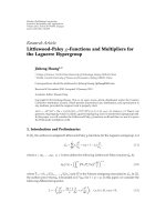
Thetopologylevelimpactsofthebodyposturevariation
are reported in Figure 3. Observe the wide swing of the node
degree (1.5 to 3.8 across the six postures/activities) which

indicates a high level of dynamism in the on-body mesh
topology. Also observe the number of simultaneous network
partitions which vary from 1 to 5, indicating frequent
topological partitioning as hypothesized in Section 1.3.As
expected, the postures with relatively lower node degree
correspond to higher number of network partitions. Such
topological disconnections necessitate on-body store-and-
forward routing.
EURASIP Journal on Wireless Communications and Networking 5
SIT REC DWN STD WLK RUN
0
1
2
3
4
Avg. node degree
0 20 40 60 80 100 120
Time (s)
0
2
4
6
No.of partitions
Avg. nodes
degree
No.of
partitions
Figure 3: Instantaneous topology and partition properties with
posture changes.
4. Topology Trace Collection for off-Body

Routing Simulation
An objective of this paper is to develop delay models
for different DTN routing protocols executed on dynamic
WBAN topologies as depicted in Figure 3.Aremotetrace
collection mechanism was developed so that real network
topology traces from the prototype WBAN can be wirelessly
collected and used for routing model development and off-
line routing simulation experiments.
As depicted in Figure 4, during the on-body experiments,
the state of each link (emulated using limited transmission
power as shown in Figure 2) is periodically sent to the out-
of-body server at full transmission power. The server collects
the link-state samples (ON or OFF) from all the on-body
links and stores them with a time-stamp from its local clock.
All these link-state samples, together, form topology traces
which are then used for delay model development and off-
body routing simulations as presented in Sections 5, 6,and
8. Results from the delay model and off-body simulations
are compared with the routing performance from the on-
body experiments since all of them use the exact same
topology traces, ensuring comparable link state and network
partitioning patterns as discussed through the example in
Figure 3.
5. Modeling DTN Routing Protocols
The objective of this section is to model the delay of (a) a
series of existing single copy DTN routing algorithms applied
to on-body settings and (b) two specific routing algorithms
that are specifically developed to leverage the locality of
WBAN topology as function of postural body movements.
Definition 1 (link state). The state of a link between two on-

body nodes i and j at the nth discrete time slot is represented
as L
i,j
(n), which is assigned the value 1 or 0 to indicate the
state to be connected or disconnected, respectively. The time
slot here is an observation time slot which corresponds to
the Hello interval period for neighbor/link discovery. In our
prototype implementation, it was set to be 1.4 sec.
Definition 2 (link disconnection probability). The Link
Disconnection Probability (LDP) for the link between node-
i and node-j is represented as

P
i,j
(k). The quantity

P
i,j
(k)
represents the probability that after an arbitrarily chosen
time slot, the link remains disconnected for k consecutive
disconnected time slots. In a sufficiently long topology trace,
spanning T time slots, if n
k
represents the number of
occurrences of such k-slot long disconnections, then the LDP
can be expressed as

P
i,j

(
k
)
=
⎧
⎪
⎪
⎨
⎪
⎪
⎩
n
k
T
,for k
≥ 1,

T
n
=1
L
i,j
(
n
)
/T,fork
= 0.
(1)
The case k
≥ 1 represents situations for which the arbitrarily

chosen slot is a part of one of the T
off
periods (except the
last slot on the T
off
period) or the last slot during one of
the T
on
periods (see Figure 5). Similarly, the case k = 0
represents situations for which the arbitrarily chosen slot is
a part of one of the T
on
periods (except the last slot on the
T
on
period) or the last slot during one of the T
off
periods.
With above definition of

P
i,j
(k), we have

T
k
=0

P
i,j

(k) = 1,
and its expected value can be represented as
ELD
i,j
=
T

k=0
k ·

P
i,j
(
k
)
,(2)
where ELD
i,j
is the Expected Link Delay, representing the
average number of disconnection slots after an arbitrarily
chosen slot. In other words, ELD
i,j
can be expressed as
ELD
i,j
= T
i,j
off
/2, where T
i,j

off
is the average disconnection
duration for link i to j.
5.1. Opportunistic Routing. In DTN opportunistic routing
(OPPT) [18–20]asourcenodedeliverspackettothe
destination node only when the two nodes come into direct
contact. This single copy mechanism offers a simple DTN
routing approach in which the delay can be very large,
especially in scenarios with low mobility or infrequent link
formation between the source and destination. This protocol
is simple to implement and suited well for the processing-
and energy-constrained on-body sensors for which complex
algorithms should be avoided. It is highly energy efficient
due to the single transmission requirement for each packet
delivery. However, the expected packet delivery delay for
OPPT can be quite high, especially when the source and the
destination nodes are rarely in direct contact with each other.
The protocol is also very sensitive to the source-destination
link quality since it relies only on that single direct link for
all packet delivery. Opportunistic routing is modeled and
analyzed in this section for estimating the worst case delay
performance and for finding an upper-bound for packet
delivery delay in a WBAN setting.
Since a source node s delivers a packet to destination d
only when L
s,d
= 1andapacketatnodes can be generated
at any arbitrary time slot, the delivery delay for a packet is
ELD
s,d

asdevelopedin(2). This is true only when the packet
generation rate is low enough so that no more than one
packet is generated during a T
off
period (see Figure 5). This
means that the generated packet can be delivered at the very
beginning of the immediately following T
on
period without
any additional wait.
6 EURASIP Journal on Wireless Communications and Networking
On-body experiment
1
2
3
5
4
7
6
Prototype WBAN
2
3
1
4
5
6
7
Real-time
topology
export

Experimental delay
performance of DTN
routing protocols
Exported dynamic topology
Offline
Simulations
Comparative
performance evaluation
Off-body
simulation
Model
performance
Figure 4: Topology export for offline and model performance.
T
ij
on
T
ij
off
Time
L
ij
:0 L
ij
:1
··· ···
Figure 5: Example connectivity of an on-body link.
However, when the packet generation rate is higher so
that multiple packets are generated during a T
off

period, the
packets need to be delivered one per time slot during the next
T
on
period. This backlog clearance adds an additional delay
component that needs to be added in addition to the ELD
s,d
from (2). Let B represent the number of packets generated
during the T
off
period. With λ being the packet generation
rate at the source node s, B
= λ·T
off
. After the subsequent T
on
period starts, these B packets are flushed one packet per time
slot, requiring B time slots. During these B slots, another B
·λ
packets are generated which are then cleared one per slot.
Combining the backlog clearance delay with the
Expected Link Delay (ELD), the average delivery delay for
the packets generated during the T
off
period can be written
as ELD
sd
+

B−1

i=1
i/B. Average delay for the packets generated
during the T
on
period can be written as B/2+

Bλ−1
i
=1
i.
Therefore, the overall average packet delay for on-body
opportunistic routing can be expressed as
D
OPPT
=

T
off
Buffered Packets ×T
off
Avg · Packet Delay

+

T
on
Buffered Packets ×T
on
Avg · Packet Delay


Total Buffered Packets
(3)
or
D
OPPT
=
B ·

ELD
sd
+

B−1
i=1
i

+ B ·λ ·

B/2+

Bλ−1
i=1
i

B + B ·λ
,
(4)
where Expected Link Delay (ELD) can be computed in (2)
and B
= λ ·T

s,d
off
= 2 ·λ ·ELD
s,d
. Note that this expression is
valid when the system is stable in the sense that on an average,
all packets generated during the T
on
and T
off
periods are able
to be delivered during the T
on
period for the link between
nodes s and d.
5.2. Randomized Routing. In randomized routing protocol
(RAND), if a node with a data packet does not have a direct
connection with the destination, the node forwards the data
packet to a neighbor chosen at random [19, 20]. The packet
is subsequently forwarded in the same way, till it is received
at the destination. Unlike for hot-potato routing [20]in
large networks, the delay performance of RAND can often
be better than that of opportunistic routing in small body
area networks only with few nodes. Smaller topologies have
lesser number of end-to-end path combinations, leading to
quicker delivery. Also, the network partitioning, as shown in
Figure 3, helps reducing the path combinations even further.
Packet looping, which is inherent in a randomized routing
protocol, can be avoided by recording a packet’s traversed
path in it incrementally so that a forwarding filtering can be

implemented. A packet is never forwarded to a node that is
recorded in that packet’s already traversed path. Like OPPT,
the randomized protocol is also simple to implement but can
deliver lower packet delay compared to OPPT. A packet being
EURASIP Journal on Wireless Communications and Networking 7
1
2
3
4
1
2
3
4
1
2
3
4
A(1) =
⎡
⎢
⎢
⎣
00.500.5
1000
0000
0010
⎤
⎥
⎥
⎦

, A(2) =
⎡
⎢
⎢
⎣
0001
0010
0000
0.50.500
⎤
⎥
⎥
⎦
, A(3) =
⎡
⎢
⎢
⎣
0010
0010
0000
0010
⎤
⎥
⎥
⎦
[A(1)·A(2)] =
⎡
⎢
⎢

⎣
0.25 0.25 0.50
0001
0000
0000
⎤
⎥
⎥
⎦
,[A(1)·A(2)·A(3)] =
⎡
⎢
⎢
⎣
000.50
0010
0000
0000
⎤
⎥
⎥
⎦
Figure 6: Example evolution of the forwarding matrix for a time-varying topology.
forwarded using the RAND protocol, however, can suffer
from a large number of unnecessary forwarding before it is
delivered at the destination. In other words, this protocol can
be quite energy-inefficient.
Definition 3 (forwarding probability). In RAND forwarding,
anode-i forwards a packet uniformly randomly to one of its
currently connected neighbors. Therefore, at any time slot

n, the probability of node i forwarding a packet to node j is
defined as
P
f
i,j
(
n
)
=
L
i,j
(
n
)

N
j
=1
L
i,j
(
n
)
, P
f
i,i
(
n
)
= 0, ∀j ∈ N,

j
/
=i, j
/
=d,if
N

j=1
L
i,j
(
n
)
/
=0, L
i,d
(
n
)
= 0,
(5)
where N is the number of nodes in the on-body network.
Equation (5)isapplicableaslongasnodei currently has
at least one neighbor (i.e.,

N
j=1
L
i,j
(n)

/
=0), and none of
those neighbors is the destination node d (i.e., L
i,d
(n) =
0). In case when node i has destination d as a current
neighbor, the packet is forwarded to node d with probability
“1”. Also, when node i has no current neighbors, it keeps
buffering the packet (i.e., P
f
i,i
(n) = 1 ), resulting in P
f
i,j
(n) =
0, for all j
/
=i. Incorporating all these situations, (5)canbe
expanded as
P
f
i,j
(
n
)
=
L
i,j
(
n

)

N
j
=1
L
i,j
(
n
)
, P
f
i,i
(
n
)
= 0, ∀j ∈ N,
j
/
=i, j
/
=d,if
N

j=1
L
i,j
(
n
)

/
=0, L
i,d
(
n
)
= 0,
P
f
i,d
(
n
)
= 1, P
f
i,i
(
n
)
= 0, P
f
i,j
(
n
)
= 0, ∀j ∈ N,
j
/
=i, j
/

=d if L
i,d
(
n
)
= 1
P
f
i,i
(
n
)
= 1, P
f
i,j
(
n
)
= 0, ∀j ∈ N,
j
/
=i,if
N

j=1
L
i,j
(
n
)

= 0.
(6)
Definition 4 (forwarding matrix). The forwarding matrix
captures the forwarding probabilities at time slot n across
all possible links in the network with N nodes and can be
represented as
A
(
n
)
=
⎡
⎢
⎢
⎢
⎢
⎢
⎢
⎢
⎢
⎢
⎢
⎢
⎢
⎢
⎢
⎢
⎢
⎢
⎢

⎢
⎢
⎢
⎣
12··· j ··· N
1: P
f
1,1
(
n
)
P
f
1,2
(
n
)
··· P
f
1,j
(
n
)
··· P
f
1,N
(
n
)
2: P

f
2,1
(
n
)
P
f
2,2
(
n
)
··· P
f
2,j
(
n
)
··· P
f
2,N
(
n
)
.
.
.
.
.
.
.

.
.
···
.
.
.
···
.
.
.
i : P
f
i,1
(
n
)
P
f
i,2
(
n
)
··· P
f
i,j
(
n
)
··· P
f

i,N
(
n
)
.
.
.
.
.
.
.
.
.
···
.
.
.
···
.
.
.
d :0 0
··· 0 ··· 0
.
.
.
.
.
.
.

.
.
···
.
.
.
···
.
.
.
N : P
f
N,1
(
n
)
P
f
N,2
(
n
)
··· P
f
N,j
(
n
)
··· P
f

N,N
(
n
)
⎤
⎥
⎥
⎥
⎥
⎥
⎥
⎥
⎥
⎥
⎥
⎥
⎥
⎥
⎥
⎥
⎥
⎥
⎥
⎥
⎥
⎥
⎦
.
(7)
The Forwarding Matrix A(n) has two notable properties.

First, the elements in the dth row are all zeros since the
destination node d never forwards a packet. The elements in
the dth column, however, are either 1 or zero (not explicitly
shown above), depending on node d’s instantaneous connec-
tivity with the other nodes as expressed above in (6). Second,
the summation of all elements in all rows (except the dth
row) should be 1. The Forwarding Matrix, which depends
on the link states L
i,j
(n), can be created after the forwarding
probabilities are computed using (6) based on the observed
link states from the collected WBAN topology traces.
Consider a data packet that is generated at node s during
the nth time slot, and delivered to node d at the (n+k)th time
slot, resulting in a delay of k slots. The value of k can vary
from 0 to infinity. Let the probability of the above event (i.e.,
delivering the packet with a delay of k slots) be represented
as the delivery probability ρ
n
s,d
(k), which can be expressed as
ρ
n
s,d
(
k
)
=
[
A

(
n
)
·A
(
n +1
)
·A
(
n + k
)
]
s,d
=


k
i
=0
A
(
n + i
)

s,d
(8)
which is the [s, d] element of the product matrix for a packet
generated at time slot i
= 0 and delivered at time i = k.
Equation (8) shows the probability of delivering a packet

with a delay of k slots, where k can range from 0 to infinity.
8 EURASIP Journal on Wireless Communications and Networking
Therefore, the expected RAND forwarding delay for a packet
that was generated at the nth time slot can be written as
D
RAND
=
T

k=0
k ·ρ
n
s,d
(
k
)
=
T

k=0
k ·


k
i
=0
A(n + i)

s,d
,(9)

where T is the length (in number of slots) of the experi-
mental topology traces obtained in Section 4. Considering
sufficiently long on-body topology traces (i.e., large T), the
maximum value of k in (9)issettobeT instead of infinity.
To clarify the above forwarding concept further, let us
explore the following example in Figure 6.Considera4-
node (i.e., N
= 4) body sensor network with node-1 as the
source and node-3 as the destination. Example forwarding
matrixes A(1), A(2), and A(3) and the corresponding
network topologies at time slots 1, 2, and 3, obtained from
the topology trace, are given in Figure 6.
Using the above matrixes, the delay probabilities can be
computed as ρ
1
1,3
(0) = 0, ρ
2
1,3
(1) = 0.5, and ρ
3
1,3
(2) = 0.5
using (8). According to A(1), at time slot 1, node-1 has two
neighbors (2 and 4), node-2 has one neighbor (node-1), and
node-4 has a direct connection with the destination node-3.
Assume that a packet is generated at source (node-1) at time
slot 1. Since node-1 has no direct connection with d (i.e.,
P
f

1,3
= 0), the packet will be randomly forwarded to either
node 2 or 4 with probability 0.5 each, but the probability of
delivering it to the destination node-3 is zero in the current
slot-1 (out of all possible infinite number of slots in future).
This is captured by ρ
1
1,3
(0) = 0 which is the [1, 3] element of
matrix A(1).
At time slot 2, the packet will be forwarded to 3 through
2 with probability 1, that is, if 2 has already received the
packet in slot 1. Otherwise (i.e., the packet was forwarded
to node 4 in slot 1), the packet will be forwarded to node-1
or node-2 by node-4 at slot 2. Therefore, the probability of
delivering the packet to the destination node-3 in slot-2 (out
of all possible slots) is 0.5. This is captured by ρ
1
1,3
(1) = 0.5
from the [1, 3] element of the product matrix [A(1)
·A(2)].
Since P
f
1,3
= P
f
2,3
= P
f

4,3
= 1inA(3), the packet is
guaranteed to be delivered to node-3 in slot-3. Since the
probability of delivery in slot-1 was zero, and in slot-2 was
0.5, and the delivery is guaranteed in slot-3 (i.e., if it was not
delivered in slot-2), the probability of delivering the packet
in slot-3 (out of all possible slots) is 0.5. In other words, the
probability of delivery with a delay of 2 slots (i.e., k
= 2) is 0.5.
This is also captured as ρ
1
1,3
(2) = 0.5 from the [1, 3] element
of the product matrix [A(1)
·A(2) ·A(3)]. Using ρ
1
1,3
(0) = 0,
ρ
1
1,3
(1) = 0.5, and ρ
1
1,3
(2) = 0.5, the expected delay for
random forwarding for this example WBAN topology trace
is 0
×0+1×0.5+2×0.5 = 1.5 time slots.
5.3. Utility-Based Routing Using Link Locality. In random-
ized routing, a node does not consider the locality of its

connectivity with other network nodes while forwarding a
packet. In utility-based routing protocols [17–21], nodes
prefer to forward packets to destination through the neigh-
bor with the latest encounter with the destination, thus
leveraging the link locality in the form of its age. Each node
is assigned a utility value based on the last encounter time
with the destination, and a packet is forwarded to a neighbor
with the highest utility value. Utility represents how useful
(fast) this node might be in delivering a data packet to the
destination and is often implemented using a timer. The
delay of utility-based routing is expected to be lower than
that in OPPT and RAND routing. Also, the number of packet
forwarding in utility-based routing is expected to be smaller
compared to RAND, mainly because of its exploitation of the
link connection locality while selecting the next-hop during
packet forwarding. The implementation of this protocol,
however, can be more complex than OPPT and RAND
because each node needs to compute and maintain the utility
information for all neighbors in the network. Therefore, for
large networks, maintaining utility information for every
node can create significant scalability concerns. However, for
small WBANs this is less of an issue because of their small
node-counts.
Let the utility function U
i,j
(n) represent the utility value,
of node i with respect to node j at the nth time slot. Every
time node i comes in contact with node j, the quantity U
i,j
(n)

is set to a maximum utility value and then for every time
slot the node remains out of contact from the destination,
the quantity U
i,j
(n) is decreased based on a preset utility
reduction method [19, 21] as a function of elapsed time. The
update rule for U
i,j
(n)canbewrittenas
U
i,j
(
n +1
)
=
⎧
⎨
⎩
U
max
,ifL
i,j
(
n +1
)
= 1,
U
i,j
(
n

)
−1, if L
i,j
(
n +1
)
= 0,
(10)
where U
max
is the maximum possible utility value to the
destination. These utility values are exchanged between
neighbors within the periodic Hello messages.
With the above definition of utility, at the nth time slot
node-i will forward a packet (destined to node-d)tonode-j
only if U
i,d
(n) <U
j,d
(n)andU
j,d
(n) ≥ U
k,d
(n), forall k ∈
ψ
i
(n), where ψ
i
(n) is the set of all neighbors of node-i during
the nth time slot.

Note that the above forwarding logic assumes that each
on-body node is guaranteed to intermittently come within
up to 2-hop contact from the destination node. In other
words, a source node is able to meet other nodes that
intermittently come in direct contact with the destination
node. In our experimental topology this assumption was
always found true [24]. In fact for a WBAN topology, it
is generally true that depending on the specific postural
patterns, all nodes intermittently form direct links with all
other nodes in the network. This observation makes the
assumption generally applicable for WBANs which usually
have a small network diameter [19, 21]. When this 2-
hop reachability assumption is not valid in large WBANS,
transitive components will need to be incorporated while
computing the utility factor.
The packet routing delay in utility-based forwarding
(UTILITY) can be computed using the same logic as in
random forwarding (RAND) except that the forwarding
probabilities P
f
i,j
(n)in(6) need to be reformulated for
EURASIP Journal on Wireless Communications and Networking 9
UTILITY. The forwarding probability in this case can be
expressed as
P
f
i,i
(
n

)
= 1, P
f
i,j
(
n
)
= 0,
∀j
/
=i ∈ N if U
i,d
(
n
)
≥ U
j,d
(
n
)
,
∀j ∈ ψ
i
(
n
)
P
f
i,j
(

n
)
= 1, P
f
i,r
(
n
)
= 0ifU
i,d
(
n
)
<U
j,d
(
n
)
,
U
j,d
(
n
)
≥ U
k,d
(
n
)
,

∀k ∈ ψ
i
(
n
)
,
∀r
/
= j ∈ N,
P
f
i,d
(
n
)
= 1, P
f
i,j
(
n
)
= 0, ∀j
/
=d ∈ N if d ∈ ψ
i
(
n
)
,
(11)

where N represents the set of all on-body nodes and where
ψ
i
(n) is the set of all neighbors of node-i during the nth
time slot. The top line of (11) represents a situation in which
either node-i does not have any neighbor during the nth time
slot, or its own utility to the destination node-d is higher
than those of all its current neighbors. Either way, the node
buffers the packet with probability 1. The middle part of the
equation codes the utility-based forwarding rule as stated
after (11). The bottom part represents the situation in which
the destination node-d is a direct neighbor of node-i, causing
a direct delivery.
Once the forwarding probabilities are computed applying
(11) on the on-body topology traces collected in Section 4,
the forwarding matrix A(n) and the delivery probabilities
ρ
n
s,d
(k) are computed using the same rules presented in (7)
and (8). Finally, the delivery delay is computed as D
UTILITY
=

T
k
=0
k ·[

k

i
=0
A(n + i)]
s,d
using (9).
5.4. Probabilistic Routing with MultiScale Postural Locality
(PRMPL). Routing using PRMPL utilizes a Postural Link
Cost (PLC) [23] which captures WBAN link localities in
multiple time scales. For on-body packet forwarding, the
PLC is used exactly the same way as for the UTILITY
routing, that is, by replacing the utility values by the PLCs.
With posture and activity changes of a human subject, the
PLC link costs are automatically adjusted such that the
packets are forwarded to next-hops which are most likely
to provide an end-to-end path with minimum intermediate
buffering/storage delays. PLC is defined as β
i,j
(n), (0 ≤
β
i,j
(n) ≤ 1), which represents the probability of finding
L
i,j
(n) = 1. The update equations for PLC are formulated
as [23, 24, 36]
β
i,j
(
n
)

= β
i,j
(
n
)
+

1 −β
i,j
(
n
−1
)

·
ω if link L
i,j
(
n
)
= 1,
β
i,j
(
n
)
= β
i,j
(
n

−1
)
·ω if link L
i,j
(
n
)
= 0.
(12)
According to (12), when the link is connected, the Postural
Link Cost (PLC) β
i,j
(n) increases at a rate determined by
the constant ω(0
≤ ω ≤ 1), and the difference between
the current value of β
i,j
(n) and its maximum value, which
is 1. As a result, if the link remains connected for a
long time, the quantity β
i,j
(n) asymptotically reaches its
maximum value of 1. When the link is disconnected, β
i,j
(n)
asymptotically reaches zero with a rate determined by the
constant ω.Tosummarize,foragivenω, β
i,j
(n) responds to
the instantaneous connectivity condition of the link L

i,j
.
With time invariant ω, the PLC update rules in (12)cap-
ture the locality in short-term link connectivity in a manner
conceptually similar to the age-based utility formulation, as
developed in [19, 21]. It is, however, not the same because in
the designs in [19, 21], the routing utility of a link is increased
incrementally when the link is formed and is reduced to
zero as soon as the link is disconnected. This formulation
of utility misses out the fact that even after disconnection,
the formation probability of that link may be higher than a
currently connected link. In other words, those definitions
of utility fairly differentiate across currently connected links,
but not across the currently nonconnected links. In the
formulation of PLC in (12), motivated by the logic used in
PROPHET [17], we track the short-term locality even when
a link is not physically connected. This extended persistency
in PLC is expected to improve performance over the existing
age-based utility definitions as used in [19, 21].
The next design step is to dimension the parameter ω for
capturing link localities at a longer time scale. From (12), the
rate of change of the PLC β
i,j
(n) per time slot can be written
as
Δ

β
i,j
(

n
)

=

1 −β
i,j
(
n
−1
)

·
ω if link L
i,j
(
n
)
= 1,
Δ

β
i,j
(
n
)

=−
β
i,j

(
n
−1
)
·
(
1
−ω
)
if link L
i,j
(
n
)
= 0.
(13)
Equation (13) indicates that for a high ω (e.g., 0.9), β
i,j
(n)
increases fast when the link is connected and decreases slowly
when the link is not connected. Conversely, for a low ω (e.g.,
0.1), β
i,j
(n) increases slowly when the link is connected and
decreases fast when the link is not connected. Ideally, it is
desirable that for a historically good link (i.e., connected
frequently on a longer time scale), β
i,j
(n) should increase
fast and decrease slowly, and for a historically bad link, it

should increase slowly and decrease fast. This implies that
the parameter ω needs to capture the long-term history of
the link; hence it should be link specific and time varying.
Based on this observation, we define Historical Connectivity
Quality (HCQ) of an on-body link L
i,j
at time slot n as
ω
i,j
(
n
)
=

n
r=n−T
window
L
i,j
(
r
)
T
window
. (14)
The constant T
window
represents a measurement window
(in number of slots) over which the connectivity quality is
averaged. The factor ω

i,j
(n), (0 ≤ ω
i,j
(n) ≤ 1), indicates
the historical link quality as a fraction of time the link
was connected during the last T
window
slots. The parameter
T
window
should be chosen based on the human postural
mobility time constants. Experimentally, we found the
optimal T
window
values that work well for a large number of
subject individuals and range of postures to be in between 7
sec. and 14 sec.
Figure 7 shows the evolution of PLC β
i,j
(n) and HCQ
ω
i,j
(n) with time. The top graph shows an example link
activity (indicated by L
ij
(n)) with the first half indicating a
10 EURASIP Journal on Wireless Communications and Networking
On
Off
L

i,j
HCQ (ω
i,j
)
PLC (B
i,j
)
0
0.2
0.4
0.6
0.8
1
0
0.2
0.4
0.6
0.8
1
0 1020 304050
ω
= 0.1
Dynamic ω
i,j
(n)
ω
= 0.9
Time slot
Figure 7: Evolution of multi-scale locality in terms of PLC and
HCQ.

steadily connected link with a single time slot (1.4 sec.) of
disconnection at time slot 10, and the second half indicates
a steadily disconnected link with single slot of connection
at the 41st slot. The top graph also shows the evolution
of ω
i,j
(n) according to (14)withaT
window
set to 7 time
slots. The bottom graph shows the evolution of β
i,j
(n)with
constant ω (i.e., 0.9 and 0.1) and link-specific time varying
ω
i,j
(n)from(14), indicating the historical link quality. When
the link is steadily well connected (during the first half), a
high constant ω (i.e., 0.9) responds well to a momentary
disconnection by decreasing β
i,j
(n) slowly, but recovering
quickly when the link becomes reconnected. A low constant
ω (i.e., 0.1) responds poorly in this situation by doing just the
opposite, that is, a fast decrease and slow recovery.
Similarly, when the link is steadily disconnected (during
the second half), a low constant ω (i.e., 0.1) responds rela-
tively better than a high constant ω (i.e., 0.9) by increasing
β
i,j
(n) slowly for a momentary connection, and decreasing

β
i,j
(n) quickly after the link becomes disconnected. The lines
for two constant ω values clearly show that a single constant
value for ω is not able to handle both good-link and bad-link
situations equally effectively.
As hypothesized, the link-specific and time-varying
β
i,j
(n), on the other hand, is able to handle both situations
well by mimicking the behavior of ω
= 0.9 during the
historically good-link situation and that of ω
= 0.1 during
the historically bad-link situation. These results clearly
demonstrate the effectiveness of the HCQ and PLC concepts
for designing routing utilities that can capture both short and
long-term localities of the on-body link dynamics. With this
multi-scale approach, the proposed mechanism should be
able to outperform both age-based (UTILITY) [19, 21]and
probabilistic [17] routing protocols that use only short-term
locality information.
Note that unlike the entities in Figures 2 and 3, the PLC
and HCQ in Figure 7 show the link connectivity localities
which depends on the short- and long-term history of the
link. The localities captures in (12)and(14) are responsible
for this memory-based behavior in Figure 7 in contrast to
the instantaneous link behavior in Figures 2 and 3. Figure 8
summarizes the structural difference between PRMPL [36]
and the UTILITY [19, 21] age-based protocol from the link

locality capture standpoint. As shown in the figure, while
UTILITY extracts only short-term locality from the link
on-off dynamics, PRMPL extracts an additional long-term
locality by observing the Historical Connectivity Quality
(HCQ) as presented in (14). Additional complexity for
PRMPL over OPPT, UTILITY, and RAND is expected due
to its periodic computation of per-link HCQ and PLC.
The forwarding rule in PRMPL is identical to what
stated for UTILITY-based forwarding in Section 5.3 with
the utility function U
i,j
(n)replaced by the postural link cost
β
i,j
(n). Consequently, the forwarding probabilities P
f
i,j
(n),
the forwarding matrix A(n), and the delivery probabilities
ρ
n
s,d
(k) can be computed using (7), (8), and (11), respectively,
and finally, the end-to-end packet delay can be computed as
D
PRMPL
=

T
k

=0
k ·[

k
i
=0
A(n + i)]
s,d
using (9).
5.5. Distance Vector Routing with Postural Link Costs (DVR-
PLC). In DVRPLC, nodes maintain end-to-end cumulative
path cost estimates to a common sink node. Let us define a
Link Cost Factor (LCF) C
i,j
(n), 0 ≤ C
i,j
(n) ≤ C
max
which
represents the routing cost for the link L
i,j
(between nodes i
and j) during the discrete time slot n. The update equations
for LCF are formulated as [23, 24, 36]
C
i,j
(
n
)
= C

i,j
(
n
−1
)
·

1 −ω
i,j
(
n
)

if link L
i,j
(
n
)
= 1,
C
i,j
(
n
)
= C
i,j
(
n
−1
)

+

C
max
−C
i,j
(
n
−1
)

·

1 −ω
i,j
(
n
)

if link L
i,j
(
n
)
= 0.
(15)
When the link is connected, C
i,j
(n) decreases at a rate
determined by (1

−ω
i,j
(n)), where ω
i,j
(n), (0 ≤ ω
i,j
(n) ≤ 1) is
the Historical Connectivity Quality, as defined in (14). If the
link remains connected for a long time, the quantity C
i,j
(n)
asymptotically reaches its minimum value 0. When the link
remains disconnected, C
i,j
(n) increases at a rate determined
by the quantity (1
− ω
i,j
(n)) and the difference between
the current cost C
i,j
(n) and its maximum value 1. This
formulation ensures that a link’s routing cost always reflects
the likelihood of the existence of the link while capturing its
historical connectivity trends. Note that the time evolution
of LCF in DVRPLC follows a rationale that is very similar
to that of PLC in PRMPL. The main difference is that while
the LCF reduces for connected links, the PLC increases in
EURASIP Journal on Wireless Communications and Networking 11
PLC

computation
model
Link status
PLC
Routing decision
Link
history
modeling
Capturing short- and long-term localities
PRMPL
Link status
Utility
Routing decision
UTILITY
Capturing short-term locality in link connectivity
Short-term
locality
L
i,j
L
i,j
Utility
function
U ( f )
Figure 8: Capturing link connectivity locality in PRMPL and UTILITY age-based routing.
such situations. Similar difference exists when a link remains
disconnected. To summarize, like in PRMPL, the cost in
DVRPC captures both short- and long-term link localities for
minimum delay packet routing.
Let γ

i,d
(n) be the minimum end-to-end cumulative cost
from node-i to the sink node-d. According to distance vector
routing logic, when a node i needs to forward a packet to the
sink node d and it meets a node j, the packet is forwarded to
node j only if the condition γ
j,d
(n) <γ
i,d
(n)isfoundtrue.In
other words, a lower path cost through node j indicates that
the latter is more likely to forward the packet to node d than
what node i’s chances are. That justifies the packet transfer
from node i to j with a goal of minimizing the end-to-end
packet routing delay.
Note that the DVRPLC protocol attempts to minimize
end-to-end cumulative routing costs. The objective is that
due to this end-to-end cost minimization, DVRPLC should
be able to outperform (from a delay standpoint) PRMPL
which always interprets its PLC only at the link level and not
in an end-to-end cumulative manner.
To execute DVRPLC, each on-body sensor node-i uses
the periodic Hello mechanism, in order to gradually develop
the C
i,j
(n) values with all other nodes in the network. It also
iteratively updates the quantity γ
i,d
(n) using the computed
C

i,j
(n) values with respect to all its neighbors. The node
then uses the Hello mechanism to send the quantityγ
i,d
(n), its
end-to-end cumulative path cost to the common destination
node-d (e.g., node 6 in Figure 1), to all other nodes that
are currently connected to node-i. This way, each node gets
updated about the path costs of all of its direct neighbors’
to the common destination node-d. The update equation for
γ
i,d
(n)
γ
i,d
(
n
)
= min

γ
i,d
(
n
)
, γ
k,d
(
n
)

+ C
i,k
(
n
)

, (16)
where node-k has the minimum γ
k,d
(n) among all the
current neighbors of node-i.
Because of its end-to-end nature, the forwarding rule in
DVRPLC is based on the end-to-end cost γ
i,d
(n)asopposed
to that based on local parameters U
i,j
(n)orβ
i,j
(n) as used
in UTILITY and PRMPL both of which do not rely on
end-to-end cost. The distance vector forwarding rule for a
packet from node-i to destination node-d can be formalized
as follows. If node-i is a direct neighbor of node-d,forward
the packet. Otherwise find node-k such that node-k has the
minimum γ
k,d
(n) among all the current neighbors of node-i.
Then forward the packet to node-k only if γ
k,d

(n) <γ
i,d
(n);
otherwise, continue buffering the node as node-i. With this
forwarding rule, the forwarding probabilities P
f
i,j
(n)canbe
expressed as
P
f
i,d
(
n
)
= 1, P
f
i,j
(
n
)
= 0, ∀j
/
=i,d ∈ N if L
i,d
(
n
)
= 1,
P

f
i,k
(
n
)
= 1, P
f
i,j
(
n
)
= 0, ∀j
/
=i,k ∈ N if L
i,d
(
n
)
/
=1,
γ
k,d
(
n
)
<γ
i,d
(
n
)

,
γ
k,d
(
n
)
≤ γ
r,d
,
∀r ∈ ψ
i
(
n
)
, r
/
=i, d, k ∈ N,
P
f
i,i
(
n
)
= 1, P
f
i,j
(
n
)
= 0, ∀j

/
=d, i ∈ N if L
i,d
(
n
)
/
=1,
γ
k,d
(
n
)
≥ γ
i,d
(
n
)
,
γ
k,d
(
n
)
≤ γ
r,d
,
∀r ∈ ψ
i
(

n
)
, r
/
=i, d, k ∈ N,
(17)
where N represents the set of all on-body nodes and where
ψ
i
(n) is the set of all neighbors of node-i during the nth
12 EURASIP Journal on Wireless Communications and Networking
time slot. The forwarding matrix A(n) and the delivery
probabilities ρ
n
s,d
(k) can be computed using (7)and(8),
respectively, and finally, the end-to-end packet delay can be
computed as D
DVRPLC
=

T
k=0
k · [

k
i=0
A(n + i)]
s,d
using

(9).
6. Routing Delay Benchmark
In order to determine the best case end-to-end delay
performance, an offline route search algorithm, Backward
Search for Delay Benchmar k Routing (BSDBR),hasbeen
developed. As long as the entire topological sequences for
a dynamically partitioned network are known a priori, the
BSDBR algorithm is able to compute the most delay optimal
end-to-end path for each packet depending on its source,
destination, time of origin, and the complete topological
sequence information. BSDBR is designed to be an offline
centralized search algorithm, to be executed in the presence
of entire time series topology information.
Let t
0
be the time instant at which a packet is generated
at node-i and routed towards destination node-d.Givena
known topology sequence, the objective is to find the earliest
time instant after t
0
at which the packet can be delivered
to the destination. Let t
1
be the earliest time instant (t
1
> t
0
) at which destination node-d comes in contact with
any other node-j (j
∈ N, j

/
=d). The minimum possible
delivery delay for the packet originated at time t
0
can be
written as (t
1
− t
0
). This minimum delay is possible only if
the necessary network links are formed across the network
during the time interval [t
0
to t
1
] so that the packet could
be forwarded multihop all the way from the origin node-i to
node-j before time t
1
. The objective of BSDBR search process
is to scan the network topology sequence in order to find if
such link formations are there so that (t
1
−t
0
)canrepresent
the minimum packet delivery delay.
If the search process concludes that the packet cannot be
delivered by time t
1

, then the next feasible time instant t
2
is
identified, and a similar search is conducted to determine if
(t
2
− t
0
) can be the minimum delivery delay. The quantity
t
2
is the earliest time instant after t
1
(t
2
> t
1
)atwhich
destination node-d comes in contact with any other node-
j (j
∈ N, j
/
=d). This BSDBR search process is iteratively
continued till a valid minimum delivery delay (t
r
− t
0
)is
found. The time instant t
r

corresponds to the earliest contact
time so that the necessary network links are formed across
the network during the time interval [t
0
to t
r
] so that the
packet can be forwarded multi-hop all the way from the
origin node-i to destination node-j by the time t
r
.
Note that the expected value of the packet delay lower
bound could have been computed using the Linear Program-
ming formulation as adopted in the full knowledge-based
approach in [28]. Instead, we have chosen to implement
BSDBR since it allows us to determine the minimum
packet delay for each individual packet as opposed to their
average in a statistical sense. Also, the formulation in [28]
is more complex than BSDBR since it incorporates the
effects of message queuing which is not studied in our
implementation.
7. Performance Evaluation
The same seven-sensor laboratory prototype network, as
shown in Figure 1, was used for the on-body experimental
evaluation of all the analyzed routing protocols. Packets
originated from all sensors were routed to the common
destination node-6, attached on the right ankle. Unless stated
otherwise, results correspond to packets originated from
node-3, representing the longest hop (i.e., also worst case)
packet routing scenario in most of the body postures. Results

are also presented from off-body simulation experiments,
carried out on network topology traces collected during the
actual on-body experiments so that the simulation results
can be compared with the experimental data for the exact
same topology traces. Those traces are also used to create the
forwarding matrix in (7) for computing the analytical packet
delay numbers for all the analyzed routing protocols.
In order to avoid the CSMA MAC collisions inherent to
Mic2Dot’s TinyOS networking stack, we have implemented a
higher-layer polling access strategy managed by one on-body
node. This polling node polls the other six-sensor nodes in a
round-robin fashion, so that a regular node forwards packets
(both data and Hello) only when it is polled by the polling
node and given access to the channel. A polling time frame
of 1.4 sec. is used which is divided into 7 time slots, one
for each of the seven on-body nodes. Note that the polling
node itself also needs to send Hello packets and so forth,
for link cost formulation as described in Section 3. Although
the data packets and the Hello messages from the nodes are
transmitted at software power-adjusted transmission range
of 0.3 m–0.6 m, the polling packets are transmitted by the
polling node at full power so that all on-body nodes receive
such packets. If a node misses a polling packet in a frame due
to channel error, it misses transmission opportunity only in
that frame.
7.1. Performance Metrics. The primary performance index is
the end-to-end Packet Delay (PD), which is modeled in this
paper and is attempted to be explicitly minimized by the
UTILITY, PRMPL, and DVRPLC protocols as presented in
Sections 5.3, 5.4,and5.5. Unlike in conventional unparti-

tioned networks, the PD in partitioned on-body networks
depends mainly on the storage delay at the intermediate
nodes. Two secondary metrics, namely, Packet Hop Count
(PHC) and Packet Delivery Ratio (PDR), are also recorded
for a more complete understanding. The index PHC captures
the number of forwarding per packet delivery, indicating the
transmission energy expenditure; it does not indicate the
packet delay since the PD in this context depends more on
the buffering/storage than on the hop-count.
7.2. Traffic Generation and Data Collection. A chosen source
node is programmed to generate data packets at the rate of 1
packet every 4 discrete time slots (each slot is 1.4 sec), with
apacketsizeof46bytes.Allon-bodynetworknodesare
slot-level time-synchronized by the sink node (i.e., node-6
in Figure 1) using periodic synchronization packet broadcast
at a high transmission power [23]. By stamping a packet
with the transmission time slot-id by the source node and
EURASIP Journal on Wireless Communications and Networking 13
2
3
4
5
6
7
1
0
2
4
6
8

10
12
Average delay (s)
OPPT. RAND. UTILity PRMPL DVRPLC BSDBR
Model
Offline
Online
41.22 42.56
43.2
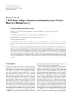
Figure 9: On-body packet delivery delay for different DTN routing protocols.
1
4.15
2.06
2.15
2.41
2.58
0
1
2
3
4
Packet hop count (PHC)
OPPT. RAND. UTILity PRMPL DVRPLC BSDBR
Figure 10: Average packet hop count.
subtracting it from the reception time slot-id at the sink
node, it is possible to compute the single-trip packet delay
(PD) at the sink node. On its way to the sink node, a data
packet collects the entire route information in the form of
a list of the intermediate node-IDs. This allows the extrac-
tion and analysis of route information including the PHC

values.
7.3. Packet Delay (PD). End-to-end packet delivery delays for
a packet from the source node-3 on left upper arm to the
sink node-6 on right ankle for all routing protocols analyzed
in Section 5 are reported in Figure 9. For each of these
protocols, a separate experiment was run for 1320 sec. (i.e.,
22 minutes), sending 230 packets, and spanning 6 different
body postures and activities (SIT, SIT-RECLINING, LYING-
DOWN, STAND, WALK, and RUN), each lasting for 20 sec.
Figure 9 reports the average of packet delay computed from
the analytical model, on-body experiment, and off-body
simulation using network topology traces collected during
the on-body experiments. The figure also shows the delay
lower-bound obtained by applying the BSDBR benchmark
algorithm (presented in Section 6) on the topology traces
collected from on-body experiments.
The following observations can be made in Figure 9.
First, the experimental, simulation, and model-generated
analytical results closely match across all protocols. Second,
as a general trend the delay performance improves with
the amount of knowledge leveraged on topological locality.
Both PRMPL and DVRPLC achieve significantly better delay
compared to the other protocols and very close to BSDBR
benchmark delay, because they are able to capture multi-
scale topological localities in human postural movements
using the cost parameters β
i,j
(n)andC
i,j
(n), as explained

in Sections 5.4 and 5.5. The age-based approach UTILITY
uses only the short-term locality, which explains its larger
delay compared to PRMPL and DVRPLC, but smaller delay
than OPPT and RAND, both of which do not leverage any
topological locality information and responds based solely
on instantaneous link conditions. Randomized forwarding
provides slightly better delay since in a typically small
WBAN, there are only few possible end-to-end path com-
binations, leading to quicker delivery than the opportunistic
14 EURASIP Journal on Wireless Communications and Networking
70
75
80
85
90
Packet delivery ratio (%)
OPPT. RAND. UTILity PRMPL DVRPLC
71%
81%
88% 88%
89%
Figure 11: Packet delivery performance observed for different protocols.
2
3
1
4
5
6
7
0

3
6
9
12
15
Average delay (s)
Src = 5 (left thigh) Src = 1(waist) Src= 3(upperleftarm)
43.2%
41.22%
OPPT. online
OPPT. model
RAND. online
RAND. model
UTILITY online
UTILITY model
PRMPL online
PRMPL model
DVRPLC online
DVRPLC model
Figure 12: Delivery delay for packets from thigh, waist, and arm to right ankle (i.e., node 6).
mode in which a delivery is possible only when the source
directly meets the destination.
7.4. Packet Hop Count (PHC). Figure 10 shows the average
PHC which serves as an indirect measure for communication
energy expenditure (i.e., for transmission and reception) for
the on-body sensors. The large number for RAND explains
the impacts of random forwarding compared to all other
protocols. The protocols DVRPLC and BSDBR take slightly
longer routes compared to the other protocols, although
those two offer better packet delays. This means that they

route packets through better quality links, leading to smaller
delays, even though it requires more number of end-to-end
hops. Since the opportunistic routing (OPPT) packets are
delivered only when a source comes in direct contact of the
destination, all packets are delivered with PHC 1.
7.5. Packet Delivery Ratio. Since no link layer packet retrans-
missions are deployed, the system is not able to recover from
the packet drops observed due to the following reason. Due
to postural mobility, there are transient blackout periods
during which a neighbor may appear to be connected in a
node’s neighbor table, when in fact it is no longer connected.
These blackout periods are created during a node’s neighbor
time-out period, which was chosen to be two polling frames
or 2.8 sec, as reported in Section 3.2. Packet transmissions
during such blackout periods end up in packet drops since no
link layer reliability is used. All five evaluated protocols suffer
from such packet losses, which are captured in the Packet
Delivery Ratio (PDR) as reported below.
In Figure 11, the poor PDR for the OPPT protocol is
caused due to a very unreliable link between the source and
the destination nodes (i.e., nodes 3 and 6 in Figure 1)which
EURASIP Journal on Wireless Communications and Networking 15
are physically situated at two extremes of the subject’s body.
Since the OPPT protocol relies on direct source-destination
contact for packet delivery, the source-destination link
quality affects this protocol most. For RAND, since the hop
count is large (see Figure 10), it is more likely for a packet
to encounter the transient blackout period during its end-
to-end trajectory, thus leading to higher drops and low
PDs. Lower hop-counts (see Figure 10) for the locality-based

protocols, namely, UTILITY, PRPML, and DVRPLC, suffer
from fewer drops due to the relatively lower occurrences of
the transient blackouts. Note that the concept of such drops
do not apply for the Benchmark case and that is why there is
no entry for BSDBR in Figure 11.
7.6. Routing Packets from and to Different Body Segments.
Delivery delays computed using the developed model and
from on-body experiment for packets from different body
segments to the sink node placed on the right ankle (i.e.,
node 6 in Figure 1) are shown in Figure 12. As shown in
the figure, the experimental and model-generated analytical
results closely match across all protocols. Observe that as
the physical distance between a source and the destination
increases, the average packet delivery delays for all the
protocols increase. Relatively though, all the experimented
routing protocols maintain the same trend for the packet
delay as observed in Section 7.2 The average packet hop-
counts from source nodes 5, 1, and 3 were experimentally
logged in the range of 1.25, 1.5, and 2.3, respectively.
Similar trends in the delivery delay were experimentally
observed for a large number of other combinations of source
and destination nodes placed at different body segments.
Although the absolute delay values were different, the overall
trend in packet delay follows the same pattern for all such
combinations that were experimented with.
7.7. Impacts of Postural Stability. For all the experiments so
far, each individual physical posture was made to last for 20
sec. In order to study the impacts of variable postural stability
on the routing performance, the subject was instructed to
repeat the same sequence of postures as in Section 3,butwith

different posture durations ranging from 10 sec. to 40 sec.
Figure 13 shows the impacts of posture duration on
average packet delay for all five protocols. Due to its
significantly higher values, the packet delays for the OPPT
protocol are plotted as a separate axis in Figure 13.Observe
that the packet delays for all the protocols generally increase
with higher posture durations. This is because longer posture
duration implies that a connected link remains connected
for longer duration and also a disconnected link remains
disconnected longer. As a result, a packet that is buffered
in a node due to network partitioning remains buffered for
longer duration, leading to higher end-to-end delay. In a
relative sense, all the experimented protocols maintain the
same performance trend for packet delay as observed in
Section 3, Figure 9. It should be observed that the packet
delays for the protocols UTILITY, PRPML, and DVRPLC
maintain very similar difference for a wide range of the
posture duration mainly because of the fact that all three of
2
6
10
14
18
Others avg. delay (s)
10 20 30 40
Posture duration (s)
10
20
30
40

50
OPPT.avg. delay (s)
OPPT.
RAND.
UTILITY
PRMPL
DVRPLC
OPPT. online
OPPT. model
RAND. online
RAND. model
UTILITY online
UTILITY model
PRMPL online
PRMPL model
DVRPLC online
DVRPLC model
Figure 13: Impacts of posture duration on packet delay.
1
3
2
5
4
7
6
Sou
rce
node
1
2

3
5
4
7
6
Sink
node
Sink
node
(P1)
(P2)
Source
node
Figure 14: Experiments with different sensor placements.
them use the link locality information, leading to the similar
trend of variation with posture duration.
7.8. Impacts of Sensor Placements. Additional on-body sensor
placements, as shown in Figure 14, were experimented with
for evaluating the validity of the routing results obtained so
far from the sensor placement shown in Figure 1.Different
source and sink nodes are used in the two placement
settings P1 and P2 in Figure 14. The inter-posture sequence,
described in Section 3.2, was followed by a subject and the
corresponding packet delay results are presented in Figure 15
for the placement settings P1 and P2 in Figure 14. Generally,
the relative performance trends across all the experimented
protocols as observed for the original sensor placement (in
Figure 9) remain valid for the new sensor placements P1 and
P2 in Figure 14. The delay for placement P1 is larger due to
the longer source-to-destination distance compared to that

in P2.
Note that the impacts of link failure were not separately
studied because the effects of such failures have already been
16 EURASIP Journal on Wireless Communications and Networking
RAND.
PRMPLUTILITY
OPPT.
DVRPLC
0
4
8
12
16
Average delay (s)
51.24 53.54:
Online
Model
(a)
RAND.
PRMPL
UTILITYOPPT.
DVRPLC
0
4
8
12
16
Average delay (s)
26.44 24.91:
Online

Model
(b)
Figure 15: On-body packet delay for (a) sensor placement P1 and (b) sensor placement P2.
captured via link disconnection in a DTN network. Also, for
a given node placement (e.g., Figures 1 and 14), the dynamic
postures (e.g., walk and run) and the variability in the
posture duration create sufficientamountofdynamismand
diversity in the network topologies, leading to a generalized
validation of the presented approach.
8. Evaluation of Node Criticality
The objective of this section is to evaluate the topological
criticality of the WBAN sensor nodes. Once identified, such
criticality information can be used for selectively reducing
the on-body sensor-count without substantially sacrificing
the packet delivery delay. The mechanism for such analysis is
to first remove all links attached to a certain number of sensor
nodes from the collected topology trace (see Section 4)and
then run off-line routing simulation experiments to evaluate
the new delay on this reduced network. Comparison between
the delays from the original trace and this reduced trace
would indicate the topological criticality of the removed
node combination from a routing standpoint.
The above mechanism is applied to the 7-node WBAN
with node-3 as the source and node-6 as the destination as
shown in Figure 1. Figure 16 shows the resulting end-to-end
packet delay characteristics when a single node (chosen from
the set 1, 2, 4, 5, or 7) is selectively removed from the network
under different routing protocols. Figure 16(a) shows the
new delay after a node is removed, and Figure 16(b) shows
the difference between the new delay and delay obtained

from the complete topology without any node removed.
The latter indicates the topological criticality of the removed
node from a routing standpoint. A positive low difference in
Figure 16(b) would indicate that the removed node is not
particularly critical for the corresponding routing protocol.
Conversely, a positive high difference would indicate that
the removed node is critical. A negative difference actually
means that the routing performance has improved after
the node is removed. This means that the corresponding
routing protocol was nonoptimally choosing the node after
removing which the routing protocol actually found a better
route, leading to lower delay. Results for all the analyzed
protocols except opportunistic routing (OPPT) are presented
in Figure 16. Since OPPT relies on direct source-destination
contact for packet delivery, removal of any intermediate node
from the topology does not impact the delivery delay, which
is why it is not included.
Observe in Figure 16(b) that removing a node from
the network creates different amount of delay difference
depending on the specific routing protocol. Note that for the
age-based UTILITY routing the delay difference is negative,
although small, when any of the nodes 1 or 2 is removed.
This indicates that UTILITY was non-optimally choosing
those two nodes and by removing any of them is forcing
the protocol to choose a better route, resulting in negative
difference. This inaccuracy is introduced by the short-term-
only connectivity locality in the protocol. On the other
hand, by leveraging both short- and long-term connectivity
locality, as introduced in Sections 5.4 and 5.5, the protocols
PRMPL and DVRPLC completely eliminate the negative

differences, which means that they always choose an optimal
route through nodes removing which actually worsens the
delay. Similarly, in Figure 16(b), the BSDBR algorithm with
benchmark delay also demonstrates optimal routes indicated
by no negative differences. Finally, observe that the node
dependencies of the RAND are generally more than those
of all other protocols mainly because with randomized
forwarding any node in WBAN can be in a packet’s path
as described in Section 5.2. In other words, since there
are no constrains on packet forwarding with the RAND
protocol,removinganynodefromtheset1,2,4,5,or7can
significantly impact the end-to-end packet delivery delay.
From the results in Figure 16(b), the following conclu-
sions can be made. First, if PRMPL or DVRPLC (these two
provide the best end-to-end delay as shown in Figure 9)is
deployed, one node from the set 1, 2, and 7 can be easily
removed without sacrificing packet delay. Second, generally,
nodes 4 and 5 are topologically more critical than all other
nodes (in the context of source 3 and destination 6) primary
EURASIP Journal on Wireless Communications and Networking 17
0
2
4
6
8
10
12
14
16
Average delay (s)

All nodes n-1 remvd. n-2 remvd. n-4 remvd. n-5 remvd. n-7 remvd.
RAND
UTILITY
PRMPL
DVRPLC
BSDBR
(a)
23
1
45
6
7
−0.6
0.4
1.4
2.4
3.4
Delay difference (s)
All nodes n-1 remvd. n-2 remvd. n-4 remvd. n-5 remvd. n-7 remvd.
RAND
UTILITY
PRMPL
DVRPLC
BSDBR
(b)
Figure 16: Single node criticality in terms of (a) packet delay and (b) packet delay difference.
because of their physical proximity to the destination and
physical placement with respect to possible routes from
node-3 to node-6.
Note that the analysis in this section shows what happens

if only one node is removed from the topology. In order to
find the impacts of removing multiple nodes, similar analysis
can be done by removing different combinations of the nodes
and then by measuring the delay differences. Also, removal
of a node will be feasible only if the primary purpose of the
node is routing and not sensing.
9. Conclusion and Ongoing Work
This paper develops a delay modeling framework for store-
and-forward packet routing in Wireless Body Area Networks
(WBANs). Using a prototype WBAN for experimentally
characterizing and capturing on-body topology traces, an
analytical delay modeling technique was developed for evalu-
ating single-copy DTN routing protocols. End-to-end rout-
ing delays for a series of protocols including opportunistic,
randomized, and two other mechanisms that capture multi-
scale topological localities in human postural movements
have been evaluated. Performance was evaluated experimen-
tally, via simulation, and using the developed models. It was
shown that via multi-scale modeling of the spatiotemporal
locality of on-body link disconnection patterns, it is possible
to attain better delay performance compared to opportunis-
tic, randomized, and utility-based DTN routing protocols
in the literature. Finally, a mechanism for evaluating the
topological importance of individual on-body sensor nodes
is developed. It is shown that such information can be used
for selectively reducing the on-body sensor-count without
18 EURASIP Journal on Wireless Communications and Networking
substantially sacrificing the packet delivery delay. Ongoing
work on this topic includes developing a Kalman Filter based
body movement prediction model for predictive on-body

packet routing with lower delay objectives.
Acknowledgments
This paper was supported by an NIH Grant 1 R21 HL093395-
01A2. Muhannad Quwaider was a Ph.D. student in Michigan
State University during this work.
References
[1] E. Jovanov, A. Milenkovic, C. Otto, and P. C. De Groen,
“A wireless body area network of intelligent motion sensors
for computer assisted physical rehabilitation,” Journal of
NeuroEngineering and Rehabilitation, vol. 2, article 6, 2005.
[2] M. Quwaider and S. Biswas, “Body posture identification
using hidden Markov model with a wearable sensor network,”
in Proceedings of the ICST 3rd International Conference on Body
Area Networks, Tempe, Ariz, USA, 2008.
[3] “WebPage of Department of Health and Human Services,”
/>[4] K. Y. Chen and D. R. Bassett Jr., “The technology of
accelerometry-based activity monitors: current and future,”
Medicine and Science in Sports and Exercise, vol. 37, no. 11, pp.
S490–S500, 2005.
[5] M. Quwaider and S. Biswas, “Physical context detection
using multi-modal sensing using wearable wireless networks,”
Journal of Communication Software and Systems, vol. 4, pp.
191–202, 2008.
[6] S. Lin, J. Zhang, G. Zhou, L. Gu, J. A. Stankovic, and T.
He, “ATPC: adaptive transmission power control for wireless
sensor networks,” in Proceedings of the 4th International
Conference on Embedded Networked Sensor Systems (SenSys
’06), pp. 223–236, ACM Press, November 2006.
[7] S. Xiao, V. Sivaraman, and A. Burdett, “Adapting radio
transmit power in wireless body area sensor networks,” in

Proceedings of the ICST 3rd Internat ional Conference on Body
Area Networks, Tempe, Ariz, USA, 2008.
[8] S. Mikami, T. Matsuno, M. Miyama, M. Yoshimoto, and H.
Ono, “A wireless-interface SoC powered by energy harvesting
for short-range data communication,” in Proceedings of the 1st
IEEE Asian Solid-State Circuits Conference (ASSCC ’05),pp.
241–244, November 2005.
[9] D. Sagan, Integrated Circuits for Medical Applications: Meeting
the Challenge of Ultra Low Power Communication,Ultra-Low-
Power Communications Division, Zarlink Semiconductor,
2005.
[10] E. Str
¨
ommer, M. Hillukkala, and A. Ylisaukkooja, “Ultra-low
Power Sensors with Near Field Communication for Mobile
Applications,” in Proceedings of the International Conference on
Wireless Network (ICWN ’07), 2007.
[11] T. Falck, H. Baldus, J. Espina, and K. Klabunde, “Plug ’n play
simplicity for wireless medical body sensors,” in Proceedings
of the Pervasive Health Conference and Workshops (Pervasive-
Health ’06), December 2006.
[12] E. Jones and P. Ward, “Routing strategies for delay-tolerant
networks,” in Proceedings of the 2006 International Conference
on Wireless Communications and Mobile Computing,Vancou-
ver, Canada, 2006.
[13] H. Guo, J. Li, Y. Qian, and Y. Tian, “A practical routing
strategy in delay tolerant networks using multiple pigeons,”
in Proceedings of IEEE Military Communications Conference
(MILCOM ’08), November 2008.
[14] J. Leguay, T. Friedman, and V. Conan, “Evaluating Moby-

Space-based routing strategies in delay-tolerant networks,”
Wireless Communications and Mobile Computing, vol. 7, no. 10,
pp. 1171–1182, 2007.
[15] V. Conan, J. Leguay, and T. Friedman, “Fixed point oppor-
tunistic routing in delay tolerant networks,” IEEE Journal on
Selected Areas in Communications, vol. 26, no. 5, Article ID
4530734, pp. 773–782, 2008.
[16]J.Leguay,T.Friedman,andV.Conan,“Evaluatingmobility
pattern space routing for DTNs,” in Proceedings of the 25th
IEEE International Conference on Computer Communications
(INFOCOM ’06), April 2006.
[17] A. Lindgren, A. Doria, and O. Schel
´
en, “Probabilistic routing
in intermittently connected networks,” ACM SIGMOBILE
Mobile Computing and Communications Review, vol. 7, no. 3,
pp. 19–20, 2003.
[18] T. Spyropoulos, K. Psounis, and C. S. Raghavendra, “Efficient
routing in intermittently connected mobile networks: the
multiple-copy case,” IEEE/AC M Transactions on Networking,
vol. 16, no. 1, pp. 77–90, 2008.
[19] T. Spyropoulos, K. Psounis, and C. S. Raghavendra, “Efficient
routing in intermittently connected mobile networks: the
single-copy case,” IEEE/ACM Transactions on Networking, vol.
16, no. 1, pp. 63–76, 2008.
[20] J. Leguay, T. Friedman, and V. Conan, “DTN routing in
a mobility pattern space,” in Proceedings of ACM SIG-
COMM Workshop on Computer Communications, pp. 276–
283, Philadelphia, Pa, USA, August 2005.
[21] H. Dubois-Ferriere, M. Grossglauser, and M. Vetterli, “Age

matters: efficient route discovery in mobile ad hoc net-
works using encounter ages,” in Proceedings of the 4th ACM
International Symposium on Mobile Ad Hoc Networking and
Computing (MOBIHOC ’03), pp. 257–266, June 2003.
[22] M. Shin, S. Hong, and I. Rhee, “DTN routing strategies
using optimal search patterns,” in Proceedings of the Annual
International Conference on Mobile Computing and Networking
(MOBICOM ’08), pp. 27–32, San Francisco, Calif, USA,
September 2008.
[23] M. Quwaider and S. Biswas, “DTN routing in body sensor net-
works with dynamic postural partitioning,” Ad Hoc Networks,
vol. 8, no. 8, pp. 824–841, 2010.
[24] M. Quwaider and S. Biswas, “Probabilistic routing in on-body
sensor networks with postural disconnections,” in Proceedings
of the 7th ACM International Symposium on Mobility Manage-
ment and Wireless Access (MobiWac ’09), pp. 149–158, Tenerife,
Spain, October 2009.
[25] C. Otto, A. Milenkovic, C. Sanders, and E. Jovanov, “System
architecture of a wireless body area sensor network for
ubiquitous health monitoring,” Journal of Mobile Multimedia,
vol. 1, pp. 307–326, 2006.
[26] B. Braem, B. Latr
´
e, I. Moerman, C. Blondia, and P. Demeester,
“The wireless autonomous spanning tree protocol for multi-
hop wireless body area networks,” in Proceedings of the 3rd
Annual International Conference on Mobile and Ubiquitous
Systems (MobiQuitous ’06), July 2006.
[27] B. Latr
´

e, B. Braem, I. Moerman et al., “A low-delay protocol for
multihopwirelessbodyareanetworks,”inProceedings of the
4th Annual International Conference on Mobile and Ubiquitous
Systems: Computing, Networking and Services (MobiQuitous
’07), August 2007.
[28] S. Jain, K. Fall, and R. Patra, “Routing in a delay tolerant
network,” in Proceedings of the ACM SIGCOMM Conference
EURASIP Journal on Wireless Communications and Networking 19
on Applications, Technologies, Architectures, and Protocols for
Computer Communications, pp. 145–157, 2004.
[29] A. Vahdat and D. Becker, “Epidemic routing for partially
connected ad hoc networks,” Tech. Rep. CS-200006, Duke
University, 2000.
[30]P.Juang,H.Oki,Y.Wang,M.Martonosi,L S.Peh,andD.
Rubenstein, “Energy-efficient computing for wildlife tracking:
design tradeoffs and early experiences with ZebraNet,” in Pro-
ceedings of the 10th International Conference on Architectural
Support for Programming Languages and Operating Systems,
pp. 96–107, October 2002.
[31] T. Spyropoulos, K. Psounis, and C. S. Raghavendra, “Spray and
wait: An efficient routing scheme for intermittently connected
mobile networks,” in Proceedings of the ACM SIGCOMM
Workshop on Delay-Tolerant Networking (WDTN ’05),pp.
252–259, 2005.
[32] S. Ni, Y. Tseng, Y. Chen, and J. Sheu, “The broadcast storm
problem in a mobile ad hoc network,” in Proceedings of the
5th annual ACM/IEEE International Conference on Mobile
Computing and Networking, pp. 151–162, Seattle, Wash, USA,
1999.
[33] A. Jindal and K. Psounis, “Performance analysis of epi-

demic routing under contention,” in Proceedings of the 2006
International Wireless Communications and Mobile Computing
Conference (IWCMC ’06), pp. 539–544, Vancouver, Canada,
July 2006.
[34] S. Burleigh, A. Hooke, L. Torgerson et al., “Delay-tolerant
networking: an approach to interplanetary internet,” IEEE
Communications Magazine, vol. 41, no. 6, pp. 128–136, 2003.
[35] M. Quwaider and S. Biswas, “Probabilistic routing in on-body
sensor networks with postural disconnections,” in Proceedings
of the 7th ACM International Symposium on Mobility Manage-
ment and Wireless Access (MobiWac’09), pp. 149–158, Tenerife,
Spain, 2009.
[36] M. Quwaider and S. Biswas, “On-body packet routing algo-
rithms for body sensor networks,” in Proceedings of the 1st
International Conference on Networks and Communications
(NetCoM ’09), pp. 171–177, December 2009.