Mobile and wireless communications physical layer development and implementation Part 1 docx
Bạn đang xem bản rút gọn của tài liệu. Xem và tải ngay bản đầy đủ của tài liệu tại đây (636.6 KB, 20 trang )
I
Mobile and Wireless Communications:
Physical layer development
and implementation
Mobile and Wireless Communications:
Physical layer development
and implementation
Edited by
Salma Ait Fares and Fumiyuki Adachi
In-Tech
intechweb.org
Published by In-Teh
In-Teh
Olajnica 19/2, 32000 Vukovar, Croatia
Abstracting and non-prot use of the material is permitted with credit to the source. Statements and
opinions expressed in the chapters are these of the individual contributors and not necessarily those of
the editors or publisher. No responsibility is accepted for the accuracy of information contained in the
published articles. Publisher assumes no responsibility liability for any damage or injury to persons or
property arising out of the use of any materials, instructions, methods or ideas contained inside. After
this work has been published by the In-Teh, authors have the right to republish it, in whole or part, in any
publication of which they are an author or editor, and the make other personal use of the work.
© 2009 In-teh
www.intechweb.org
Additional copies can be obtained from:
First published January 2010
Printed in India
Technical Editor: Zeljko Debeljuh
Mobile and Wireless Communications: Physical layer development and implementation,
Edited by Salma Ait Fares and Fumiyuki Adachi
p. cm.
ISBN 978-953-307-043-8
V
Preface
Mobile and Wireless Communications have been one of the major revolutions of the late
twentieth century. We are witnessing a very fast growth in these technologies where mobile
and wireless communications have become so ubiquitous in our society and indispensable
for our daily lives. The relentless demand for higher data rates with better quality of services
to comply with state-of-the art applications has revolutionized the wireless communication
eld and led to the emergence of new technologies such as Bluetooth, WiFi, Wimax, Ultra
wideband, OFDMA. Moreover, the market tendency conrms that this revolution is not
ready to stop in the foreseen future.
Mobile and wireless communications applications cover diverse areas including entertainment,
industrialist, biomedical, medicine, safety and security, and others, which denitely are
improving our daily life. Wireless communication network is a multidisciplinary eld
addressing different aspects raging from theoretical analysis, system architecture design,
and hardware and software implementations. While different new applications are requiring
higher data rates and better quality of service and prolonging the mobile battery life, new
development and advance research studies and systems and circuits design are necessary
to keep pace with the market requirements. This book covers the most advanced research
and development topics in mobile and wireless communication networks. It is divided into
two parts with a total of thirty-four stand-alone chapters covering various areas of wireless
communications of special topics including: physical layer and network layer, access methods
and scheduling, techniques and technologies, antenna and amplier design, integrate circuit
design, applications and systems. These chapters present advanced novel and cutting-
edge results and development related to wireless communication offering the readers the
opportunity to enrich their knowledge in specic topics as well as to explore the whole eld
of rapidly emerging mobile and wireless networks. We hope that this book will be useful for
the students, researchers and practitioners in their research studies.
This rst part of the book addresses mainly the physical layer design of mobile and wireless
communication and consists of sixteen chapters classied in four corresponding sections:
1.PropagationMeasurementsandChannelCharacterizationandModeling.
2.MultipleAntennaSystemsandSpace-TimeProcessing.
3.OFDMSystems.
4.ModelingandPerformanceCharacterization.
VI
The rst section contains three chapters related to Propagation Measurements and Channel
Characterization and Modeling. The focus of the contributions in this section, are channel
characterization in tunnels wireless communication, novel approach to modeling MIMO
wireless communication channels and a review of the high altitude platforms technology.
The second section contains ve chapters related to Multiple Antenna Systems and Space-
Time Processing. The focus of the contributions in this section, are new beamforming and
diversity combining techniques, and space-time code techniques for MIMO systems.
The third section contains four chapters related to OFDM Systems. This section addresses
frequency-domain equalization technique in single carrier wireless communication systems,
advanced technique for PAPR reduction of OFDM Signals and subcarrier allocation in
OFDMA in cellular and relay networks.
The forth section contains four chapters related to Modeling and Performance Characterization.
In this section, a unied data and energy model for wireless communication and a new system
level mathematical performance analysis of mobile cellular CDMA networks are presented.
In addition, novel approach to modeling MIMO wireless communication channels and a
review of the in high altitude platforms technology are proposed.
Section 1: Propagation Measurements and Channel Characterization and modeling
Chapter 1 presents a review of the theoretical early and recent studies done on communication
within tunnels. The theory of mode propagation in straight tunnels of circular, rectangular and
arched cross sections has been studied. Comparison of the theory with existing experimental
measurements in real tunnels has been also covered.
Chapter 2 reviews the applications of the Thomson Multitaper, for problems encountered in
communications. In particular it focuses on issues related to channel modeling, estimation
and prediction for MIMO wireless communication channels.
Chapter 3 presents an overview of the HAP (High Altitude Platforms) concept development
and HAP trails to show the worldwide interest in this emerging novel technology. A
comparison of the HAP system has been given based on the basic characteristics of HAP,
terrestrial and satellite systems.
Section 2: Multiple antenna systems and space-time processing
Chapter 4 discusses the performance analysis of wireless communication systems where the
receiver is equipped with maximal–ratio–combining (MRC), for performance improvement,
in the Nakagami-m fading environment.
Chapter 5 presents a new approach using sequential blind beamforming to remedy both the
inter-symbol interference and intra-symbol interference problems in underground wireless
communication networks using jointly CMA, LMS and adaptive fractional time delay
estimation ltering.
Chapter 6 examines the possibility of multiple HAP (High Altitude Platforms) coverage of
a common cell area in WCDMA systems with and without space-time diversity techniques.
Chapter 7 presents an overview of space-time block codes, with a focus on hybrid codes, and
analyzes two hybrid MIMO space-time codes with arbitrary number of STBC/ABBA and
spatial layers, and a receiver algorithm with very low complexity.
VII
Chapter 8 discusses the MIMO channel performance in the LOS environment, classied into
two cases: the pure LOS propagation and the LOS propagation with a typical scatter. The
MIMO channel capacity and the condition number of the matrix were also investigated.
Section 3: OFDM Systems
Chapter 9 proposes an iterative optimization method of transmit/receive frequency domain
equalization (TR-FDE) based on MMSE criterion, where both transmit and receive FDE
weights are iteratively determined with a recursive algorithm so as to minimize the mean
square error at a virtual receiver.
Chapter 10 proposes an enhanced version of the iterative ipping algorithm to efciently
reduce the PAPR of OFDM signal.
Chapter 11 discusses the problem of allocating resources to multiple users on the downlink
in an LTE (Long Term Evolution) cellular communication system in order to maximize
system throughput. A reduced complexity sub-optimal scheduler was proposed and found
to perform quite well relative to the optimal scheduler.
Chapter 12 introduces the DTB (distributed transmit beamforming) approach to JCDS
(joint cooperative diversity and scheduling) OFDMA-based relay network in multi source-
destination pair’s environment and highlights its potential to increase the diversity order and
the system throughput performance. In addition, to trade-off a small quantity of the system
throughput in return for signicant improvement in the user throughput, a xed cyclic delay
diversity approach has been introduced at relay stations to the proposed JCDS-DTB.
Section 4: Modeling and Performance Characterization
Chapter 13 presents the mathematical analysis of mobile cellular CDMA networks considering
link unreliability in a system level analysis. Wireless channel unreliability was modeled by
means of a Poisson call interruption process which allows an elegant teletrafc analysis
considering both wireless link unreliability and resource insufciency.
Chapter 14 presents a developed energy model to conduct simulations which describe the
energy consumption by sending a well dened amount of data over a wireless link with
xed properties. The main aim in this study was to maximize the amount of successfully
transmitted data in surroundings where energy is a scarce resource.
Chapter 15 reviews the performance strengths and weaknesses of various short range
wireless communications e.g. RadioMetrix, IEEE 802.11a/b, IEEE 802.15.4, DECT, Linx, etc,
which are commonly used nowadays in different RoboCup SSL wireless communication
implementations. An adaptive error correction and frequency hopping scheme has been
proposed to improve its immunity to interference and enhance the wireless communication
performance.
Chapter 16 reviews the capacity dimensioning methods exploited for system capacity
performance evaluation and wireless network planning used in development process of any
generation of mobile communications system.
VIII
Editors
Salma Ait Fares
GraduateSchoolofEngineering
DepartmentofElectricalandCommunicationEngineering
TohokuUniversity,Sendai,Japan
Email:
Fumiyuki Adachi
GraduateSchoolofEngineering
DepartmentofElectricalandCommunicationEngineering
TohokuUniversity,Sendai,Japan
Email:
IX
Contents
Preface V
Section 1: Propagation Measurements and Channel Characterization and modeling
1. WirelessTransmissioninTunnels 011
SamirF.Mahmoud
2. WirelessCommunicationsandMultitaperAnalysis:ApplicationstoChannel
ModellingandEstimation 035
SaharJavaherHaghighi,SergueiPrimak,ValeriKontorovichandErvinSejdić
3. HighAltitudePlatformsforWirelessMobileCommunicationApplications 057
ZheYangandAbbasMohammed
Section 2: Multiple antenna systems and space-time processing
4. PerformanceofWirelessCommunicationSystemswithMRCoverNakagami–m
FadingChannels 067
TuanA.TranandAbuB.Sesay
5. SequentialBlindBeamformingforWirelessMultipathCommunicationsin
ConnedAreas 087
SalmaAitFares,TayebDenidni,SoeneAffesandCharlesDespins
6. Space-TimeDiversityTechniquesforWCDMAHighAltitudePlatformSystems 113
AbbasMohammedandTommyHult
7. High-Rate,ReliableCommunicationswithHybridSpace-TimeCodes 129
JoaquínCortezandMiguelBazdresch
8. MIMOChannelCharacteristicsinLine-of-SightEnvironments 157
LeileiLiu,WeiHong,NianzuZhang,HaimingWangandGuangqiYang
Section 3: OFDM Systems
9. IterativeJointOptimizationofTransmit/ReceiveFrequency-DomainEqualization
inSingleCarrierWirelessCommunicationSystems 175
XiaogengYuan,OsamuMutaandYoshihikoAkaiwa
X
10. AnEnhancedIterativeFlippingPTSTechniqueforPAPRReductionofOFDM
Signals 185
ByungMooLeeandRuiJ.P.deFigueiredo
11. DownlinkResourceSchedulinginanLTESystem 199
RaymondKwan,CyrilLeungandJieZhang
12. JointCooperativeDiversityandSchedulinginOFDMARelaySystem 219
SalmaAitFares,FumiyukiAdachiandEisukeKudoh
Section 4: Modeling and Performance Characterization
13. PerformanceModellingandAnalysisofMobileWirelessNetworks 237
CarmenB.Rodríguez-Estrello,GenaroHernándezValdezandFelipeA.CruzPérez
14. AUniedDataandEnergyModelforWirelessCommunicationwithMoving
SendersandFixedReceivers 261
ArminVeichtlbauerandPeterDornger
15. TowardsPerformanceEnhancementofShortRangeWirelessCommunications
inReliability-andDelay-CriticalApplications 279
YangLiu and Ye Liu
16. CapacityDimensioningforWirelessCommunicationsSystem 293
XinshengZhaoandHaoLiang
WirelessTransmissioninTunnels 1
WirelessTransmissioninTunnels
SamirF.Mahmoud
X
Wireless Transmission in Tunnels
Samir F. Mahmoud
Kuwait University
Kuwait
1. Introduction
Study of electromagnetic wave propagation within tunnels was driven in the early seventies
by the need for communication among workers in mine tunnels. Such tunnels are found in
the form of a grid of crossing tunnels running for several kilometers, which called for
reliable means of communication. Since then a great number of contributions have appeared
in the open literature studying the mechanisms of communication in tunnels. Much
experimental and theoretical work was done in USA and Europe concerning the
development of wireless and wire communication in tunnels. A typical straight tunnel with
cross sectional linear dimensions of few meters can act as a waveguide to electromagnetic
waves at UHF and the upper VHF bands; i.e. at wavelengths in the range of a fraction of a
meter to few meters. In this range, a tunnel is wide enough to support free propagation of
electromagnetic waves, hence provides communication over ranges of up to several
kilometers. At those high frequencies, the tunnel walls act as good dielectric with small loss
tangent. For example at a frequency of 1000 MHz, the rocky wall with 10
-2
Siemens/m
conductivity and relative permittivity of about 10 has a loss tangent equal to 0.018. So the
electromagnetic wave losses will be caused mainly by radiation or refraction through the
walls with little or negligible ohmic losses as deduced by Glaser (1967, 1969).
Goddard (1973) performed some experiments on UHF and VHF wave propagation in mine
tunnels in USA. His work was presented in the Thru-Earth Workshop held in Golden,
Colorado in August 1973. Goddard’s experimental results show that small attenuation is
attained in the UHF band. He also measured wave losses around corners and detected high
coupling loss between crossing tunnels. The theory of mode propagation of electromagnetic
waves in tunnels of rectangular cross section was reported by Emslie et al (1973) in the same
workshop and later in (1975) in the IEEE, AP journal. Their presentation extended the theory
given earlier by (Marcatelli and Schmeltzer, 1964) and have shown, among other things, that
the modal attenuation decreases with the applied frequency squared. Chiba et al. (1978)
presented experimental results on the attenuation in a tunnel with a cross section close to
circular except for a flat base. They have shown that the measured attenuation closely match
the theoretical attenuation of the dominant modes in a circular tunnel of equal cross section.
Mahmoud and Wait (1974a) applied geometrical ray theory to obtain the fields of a dipole
source in a tunnel with rectangular cross section of linear dimensions of several
wavelengths. The same authors (Mahmoud and Wait, 1974b) studied the attenuation in a
1
MobileandWirelessCommunications:Physicallayerdevelopmentandimplementation2
curved rectangular tunnel showing a considerable increase in attenuation due to the
curvature.
Recent advances on wireless communication, in general, have revived interest in continued
studies of free electromagnetic transmission in tunnels. Notable contributions have been
made by Donald Dudley in USA and Pierre Degauque in France and their research teams.
In the next sections, we review the theoretical early and recent studies done on
communication within tunnels. We start by reviewing the mode theory of propagation in a
straight tunnel model with a circular cross-section. We obtain the propagation parameters of
the important lower order modes in closed forms. Such modes dominate the total field at
sufficiently distant points from the source. We follow by reviewing mode propagation in
tunnels with rectangular cross section. Tunnels with arched cross sections are then treated
as perturbed tunnel shapes using the perturbation theory to characterize their dominant
modes. We also review studies made on wave propagation in curved tunnels and
propagation around corners. We conclude by comparisons between theory and available
experimental results.
2. Tunnel wall Characterization
Before treating modal propagation in tunnels, it will prove useful to characterize the tunnel
wall as constant impedance surfaces for the dominant modes of propagation. This is
covered in detail in [Mahmoud, 1991, chapter 3] for planar and cylindrical guides. Here we
give a simplified argument for adopting the concept of constant impedance wall. By this
term, we mean that the surface impedance of the wall is almost independent of the angle of
wave incidence onto the wall. So, let us consider a planar surface separating the tunnel
interior (air) from the wall medium with relative permittivity
r
and permeability
0
where
r
is usually >>1. At a given applied angular frequency , the bulk wavenumber in air is
0 0 0
k
and in the wall is
0 0r
k k k
. We may define three right handed
mutually orthogonal unit vectors
ˆ
ˆ
ˆ
, ,n t z where
ˆ
ˆ
andt z
are tangential to the air-wall interface
and
ˆ
n
is normal to the interface and is directed into the wall. Now consider a wave that
travels along the interface with dependence
exp( )j t j z
in both the air and wall. For
modes with
0
k
, one has
2 2 2
0 0
k k
and definitely
2 2 2
0
k k
. Hence the transverse
wavenumber in the wall (along
ˆ
n
)
2 2
n
k k
can be well approximated by the
2 2
0n
k k k which is independent of
. If the wave is TE
n
polarized , i.e. having zero E
n
and nonzero H
n
, the surface impedance of the wall is given by:
2 2
0 0 0
/ / / 1
s t z r
Z E H k k
(1)
Similarly if the wave is TM
n
polarized, the surface admittance of the wall is
2 2
0 0
/ / / 1
s t z r r
Y H E k k
(2)
where
0
is the wave impedance in air(=120 ).
The Z
s
and Y
s
in (1-2) are the constant impedance/admittance of the wall. When the air-wall
interface is of cylindrical shape, the same Z
s
and Y
s
apply provided that
2 2 1/ 2
0
( ) 1k k a
([Mahmoud, 1991), where a is the cylinder radius. This condition is
satisfied in most tunnels at the operating frequencies.
Fig. 1. A circular cylindrical tunnel of radius ‘a’ in a host medium of relative permittivity
r
and conductivity ‘
’.
3. Modal propagation in a tunnel with a circular cross Section
An empty tunnel with a circular cross section is depicted in Figure 1. The surrounding
medium has a relative permittivity
r
(assumed >>1) and conductivity
S/m. The circular
shape allows for rigorous treatment of the free propagating modes. The modal equation for
the various propagating modes was derived by Stratton [1941] and solved approximately
for the modal phase and attenuation constants of the low order modes in (Marcatili and
Shmeltzer, 1964), (Glasier, 1969) and more recently by Mahmoud (1991). In the following,
we derive modal solutions that are quite accurate as long as the tunnel diameter is large
relative to the applied wavelength. Under these conditions the tunnel wall is characterized
by the constant surface impedance and admittance given in (1-2). Specialized to the circular
tunnel, they take the form:
0 0
and
s
z s z
E Z H H Y E
(3)
Here
and
s
s
Z
Y are normalized impedance and admittance relative to
0
and
0
-1
respectively. Explicitly:
0
1/ 1 / ,
s r
Z i
(4a)
0 0
( / ) / 1 /
s r r
Y i i
(4b)
a
a
r
,
WirelessTransmissioninTunnels 3
curved rectangular tunnel showing a considerable increase in attenuation due to the
curvature.
Recent advances on wireless communication, in general, have revived interest in continued
studies of free electromagnetic transmission in tunnels. Notable contributions have been
made by Donald Dudley in USA and Pierre Degauque in France and their research teams.
In the next sections, we review the theoretical early and recent studies done on
communication within tunnels. We start by reviewing the mode theory of propagation in a
straight tunnel model with a circular cross-section. We obtain the propagation parameters of
the important lower order modes in closed forms. Such modes dominate the total field at
sufficiently distant points from the source. We follow by reviewing mode propagation in
tunnels with rectangular cross section. Tunnels with arched cross sections are then treated
as perturbed tunnel shapes using the perturbation theory to characterize their dominant
modes. We also review studies made on wave propagation in curved tunnels and
propagation around corners. We conclude by comparisons between theory and available
experimental results.
2. Tunnel wall Characterization
Before treating modal propagation in tunnels, it will prove useful to characterize the tunnel
wall as constant impedance surfaces for the dominant modes of propagation. This is
covered in detail in [Mahmoud, 1991, chapter 3] for planar and cylindrical guides. Here we
give a simplified argument for adopting the concept of constant impedance wall. By this
term, we mean that the surface impedance of the wall is almost independent of the angle of
wave incidence onto the wall. So, let us consider a planar surface separating the tunnel
interior (air) from the wall medium with relative permittivity
r
and permeability
0
where
r
is usually >>1. At a given applied angular frequency , the bulk wavenumber in air is
0 0 0
k
and in the wall is
0 0r
k k k
. We may define three right handed
mutually orthogonal unit vectors
ˆ
ˆ
ˆ
, ,n t z where
ˆ
ˆ
andt z
are tangential to the air-wall interface
and
ˆ
n
is normal to the interface and is directed into the wall. Now consider a wave that
travels along the interface with dependence
exp( )j t j z
in both the air and wall. For
modes with
0
k
, one has
2 2 2
0 0
k k
and definitely
2 2 2
0
k k
. Hence the transverse
wavenumber in the wall (along
ˆ
n
)
2 2
n
k k
can be well approximated by the
2 2
0n
k k k which is independent of
. If the wave is TE
n
polarized , i.e. having zero E
n
and nonzero H
n
, the surface impedance of the wall is given by:
2 2
0 0 0
/ / / 1
s t z r
Z E H k k
(1)
Similarly if the wave is TM
n
polarized, the surface admittance of the wall is
2 2
0 0
/ / / 1
s t z r r
Y H E k k
(2)
where
0
is the wave impedance in air(=120 ).
The Z
s
and Y
s
in (1-2) are the constant impedance/admittance of the wall. When the air-wall
interface is of cylindrical shape, the same Z
s
and Y
s
apply provided that
2 2 1/ 2
0
( ) 1k k a
([Mahmoud, 1991), where a is the cylinder radius. This condition is
satisfied in most tunnels at the operating frequencies.
Fig. 1. A circular cylindrical tunnel of radius ‘a’ in a host medium of relative permittivity
r
and conductivity ‘
’.
3. Modal propagation in a tunnel with a circular cross Section
An empty tunnel with a circular cross section is depicted in Figure 1. The surrounding
medium has a relative permittivity
r
(assumed >>1) and conductivity
S/m. The circular
shape allows for rigorous treatment of the free propagating modes. The modal equation for
the various propagating modes was derived by Stratton [1941] and solved approximately
for the modal phase and attenuation constants of the low order modes in (Marcatili and
Shmeltzer, 1964), (Glasier, 1969) and more recently by Mahmoud (1991). In the following,
we derive modal solutions that are quite accurate as long as the tunnel diameter is large
relative to the applied wavelength. Under these conditions the tunnel wall is characterized
by the constant surface impedance and admittance given in (1-2). Specialized to the circular
tunnel, they take the form:
0 0
and
s
z s z
E Z H H Y E
(3)
Here
and
s
s
Z
Y are normalized impedance and admittance relative to
0
and
0
-1
respectively. Explicitly:
0
1/ 1 / ,
s r
Z i
(4a)
0 0
( / ) / 1 /
s r r
Y i i
(4b)
a
a
r
,
MobileandWirelessCommunications:Physicallayerdevelopmentandimplementation4
Because of the imperfectly reflecting walls, the allowed modes are generally hybrid with
nonzero longitudinal field components E
z
and H
z
(Mahmoud, 1991, sec. 3.4). Thus:
( )sin exp
z n
E jJ k n j z
(5a)
0
( )cos exp
z n
H j J k m j z
(5b)
where
is the mode hybrid factor,
is the mode propagation factor, J(.) is the Bessel
function of first kind, and n is an integer =0,1,2…. The transverse fields
, , ,E E H and H
are obtainable in terms of the longitudinal components through well-known relations as
given in the Appendix. The boundary conditions at the tunnel wall
=a require
that
0 0
and
s
z s z
E Z H H Y E
. Using (A2) & A(3) in the Appendix along with (5), these
boundary conditions read:
2
0
( ) / v /
s
F
u jZ u n k
(6a)
2
0
( ) / v /
s
F
u jY u n k
(6b)
where:
0
2 2 2
1 1
1 1
, v ,
v ( ) , and
( ) ( ) ( )
( )
( ) ( ) ( )
n n n
n
n n n
u k a k a
u a
u J u J u J u
F u n
J
u J u J u
(7)
The prime denotes differentiation with respect to the argument and the last equality stems
from identities in (A4).
Equations (6) lead to the modal equation for the propagation factor
and themode hybrid
factor
. Namely:
2 2 2 2
0
( ( ) / v)( ( ) / v) ( / ) 0
n s n s
F u ju Y F u ju Z n k
(8a)
1 2
0
( ) / v
s s
j
Y Z u k n
(8b)
3.1 The - symmetric modes (n=0)
Considering first the
-symmetric modes we set n=0 in (8) which then reduces to two
equations for the TM
0m
and TE
0m
modes; namely:
2
0 1 0
( ) ( ) / ( ) / v
s
F u uJ u J u ju Y (9a)
2
0 1 0
( ) ( ) / ( ) / v
s
F u uJ u J u ju Z (9b)
For the low order modes which are dominant at sufficiently high frequencies, u/v <<1,
hence the RHS of (9a-9b) are also <<1 and an approximate solution for the eigenvalue u is:
0 1
(1 / v )
m m s
u x jY (10)
0 1
(1 / v )
m m s
u x jZ (11)
for TM
0m
and TE
0m
respectively. In the above x
1m
is the mth root of the Bessel function J
1
.
Note that the second of (8) yields
=0 (H
z
=0) or infinity (E
z
=0) as expected for the TM
0
and
TE
0
modes respectively. Since
2 2
a v u
, we can use (10-11) to get the complex factor.
Of particular interest are the modal attenuation rates, which take the forms
2
1
0
2 3
0
Re
s
m
m
s
Z
x
Y
k a
Neper/m (12)
The TE
0
modes are associated with Z
s
and the TM
0
modes with Y
s
. Since
s
s
Z
Y
(see (4)), it
is clear that the TE
0
modes have considerably less attenuation than the TM
0
modes; it is less
by almost the factor
r
.
3.2 Hybrid Modes
Next we consider the case n>0 for the hybrid modes. In the high frequency regime and for
the low order modes, we use the following approximations in (8): (/k
0
)
2
~ 1, and u
2
/v<<1.
This leads to the approximate solutions:
1,
(1 ( )/ 2v )
nm n m s s
u x j Z Y
(13)
and
1,
(1 ( )/ 2v )
nm n m s s
u x j Z Y
(14)
The corresponding modes are designated as HE
nm
and EH
nm
modes respectively.
Investigating the hybrid factor
(the second of eqn. 8), we find that it approaches +1 for HE
and -1 for EH modes in the infinite frequency limit. This means that the modes are hybrid
balanced modes in this limit. Further discussions on these modes are found in
(Mahmoud,1991, Chap.5).
Using (13)-(14) along with the relation
2 2
a v u
, we obtain the high frequency modal
propagation constant. Again, the imaginary part of
gives the mode attenuation rate
(=-
Im(
)). The approximate modal attenuation factor
for the HE
nm
modes is:
2
1,
2 3
0
Re
2
n m
nm s s
x
Y Z
k a
(Neper/m) (15)
The attenuation rate for the other set of modes; EH
nm
modes, is the same except that the
Bessel root x
n-1,m
is replaced by x
n+1,m
. The above formulae (12 and 15) show that the modal
attenuation is inversely proportional to the frequency squared and the radius cubed. Note
WirelessTransmissioninTunnels 5
Because of the imperfectly reflecting walls, the allowed modes are generally hybrid with
nonzero longitudinal field components E
z
and H
z
(Mahmoud, 1991, sec. 3.4). Thus:
( )sin exp
z n
E jJ k n j z
(5a)
0
( )cos exp
z n
H j J k m j z
(5b)
where
is the mode hybrid factor,
is the mode propagation factor, J(.) is the Bessel
function of first kind, and n is an integer =0,1,2…. The transverse fields
, , ,E E H and H
are obtainable in terms of the longitudinal components through well-known relations as
given in the Appendix. The boundary conditions at the tunnel wall
=a require
that
0 0
and
s
z s z
E Z H H Y E
. Using (A2) & A(3) in the Appendix along with (5), these
boundary conditions read:
2
0
( ) / v /
s
F
u jZ u n k
(6a)
2
0
( ) / v /
s
F
u jY u n k
(6b)
where:
0
2 2 2
1 1
1 1
, v ,
v ( ) , and
( ) ( ) ( )
( )
( ) ( ) ( )
n n n
n
n n n
u k a k a
u a
u J u J u J u
F u n
J
u J u J u
(7)
The prime denotes differentiation with respect to the argument and the last equality stems
from identities in (A4).
Equations (6) lead to the modal equation for the propagation factor
and themode hybrid
factor
. Namely:
2 2 2 2
0
( ( ) / v)( ( ) / v) ( / ) 0
n s n s
F u ju Y F u ju Z n k
(8a)
1 2
0
( ) / v
s s
j
Y Z u k n
(8b)
3.1 The - symmetric modes (n=0)
Considering first the
-symmetric modes we set n=0 in (8) which then reduces to two
equations for the TM
0m
and TE
0m
modes; namely:
2
0 1 0
( ) ( ) / ( ) / v
s
F u uJ u J u ju Y (9a)
2
0 1 0
( ) ( ) / ( ) / v
s
F u uJ u J u ju Z (9b)
For the low order modes which are dominant at sufficiently high frequencies, u/v <<1,
hence the RHS of (9a-9b) are also <<1 and an approximate solution for the eigenvalue u is:
0 1
(1 / v )
m m s
u x jY (10)
0 1
(1 / v )
m m s
u x jZ (11)
for TM
0m
and TE
0m
respectively. In the above x
1m
is the mth root of the Bessel function J
1
.
Note that the second of (8) yields
=0 (H
z
=0) or infinity (E
z
=0) as expected for the TM
0
and
TE
0
modes respectively. Since
2 2
a v u
, we can use (10-11) to get the complex factor.
Of particular interest are the modal attenuation rates, which take the forms
2
1
0
2 3
0
Re
s
m
m
s
Z
x
Y
k a
Neper/m (12)
The TE
0
modes are associated with Z
s
and the TM
0
modes with Y
s
. Since
s
s
Z
Y (see (4)), it
is clear that the TE
0
modes have considerably less attenuation than the TM
0
modes; it is less
by almost the factor
r
.
3.2 Hybrid Modes
Next we consider the case n>0 for the hybrid modes. In the high frequency regime and for
the low order modes, we use the following approximations in (8): (/k
0
)
2
~ 1, and u
2
/v<<1.
This leads to the approximate solutions:
1,
(1 ( )/ 2v )
nm n m s s
u x j Z Y
(13)
and
1,
(1 ( )/ 2v )
nm n m s s
u x j Z Y
(14)
The corresponding modes are designated as HE
nm
and EH
nm
modes respectively.
Investigating the hybrid factor
(the second of eqn. 8), we find that it approaches +1 for HE
and -1 for EH modes in the infinite frequency limit. This means that the modes are hybrid
balanced modes in this limit. Further discussions on these modes are found in
(Mahmoud,1991, Chap.5).
Using (13)-(14) along with the relation
2 2
a v u
, we obtain the high frequency modal
propagation constant. Again, the imaginary part of
gives the mode attenuation rate
(=-
Im(
)). The approximate modal attenuation factor
for the HE
nm
modes is:
2
1,
2 3
0
Re
2
n m
nm s s
x
Y Z
k a
(Neper/m) (15)
The attenuation rate for the other set of modes; EH
nm
modes, is the same except that the
Bessel root x
n-1,m
is replaced by x
n+1,m
. The above formulae (12 and 15) show that the modal
attenuation is inversely proportional to the frequency squared and the radius cubed. Note
MobileandWirelessCommunications:Physicallayerdevelopmentandimplementation6
that these Formulae are restricted to the lower order modes of the tunnel at sufficiently high
frequencies.
It is clear that the least attenuated mode of the TE
0
and TM
0
mode group is the TE
01
mode,
while the least attenuated hybrid mode is the HE
11
mode. It is interesting to compare the
attenuation rates of these two modes; namely the TE
01
and the HE
11
mode. Using (12) and
(15), we get the ratio
2
2
1,1
01
2 2
11
0,1
2 3.832 2 5.078
1 1 1
2.405
TE
HE r r r
x
x
(16)
where we have neglected the earth conductivity
relative to
. As an example, for typical
earth with
r
=12, the above ratio amounts to 0.395, which means that the TE
01
mode is the
least attenuated mode in a typical circular tunnel.
In order to check the approximate closed forms (12)-(15) for the attenuation factors, we
compare them with exact results presented recently by Dudley and Mahmoud [2006] in
Table 1. The table lists the attenuation rates of some of the dominant modes in a circular
tunnel of 2 meter radius and outer medium having
r
=12 at 1 GHz. It is seen that the
percentage error is less than ~2.7% for all the listed modes except the EH
11
mode. This mode
requires a higher frequency for the approximate attenuation to have a better accuracy.
Mode
Exact
Approximate
% Error
TE
01
1.098 1.096 0.18%
TE
02
3.716 3.673 1.16%
TE
03
7.937 7.724 2.68 %
HE
11
2.774 2.805 1.12%
HE
21
7.158 7.122 0.50%
HE
31
13.12 12.79 2.52%
TM
01
13.30 13.15 1.13%
EH
11
20.18 12.794 36.6%
Table 1. Comparison between Exact [Dudley & Mahmoud,2006] and approximate
attenuation rates in dB/100meters at 1 GHz.
Exercise 1: Verify the approximate attenuation rates in Table 1, Column 3 by using (12) for
the TE
0m
/TM
0m
modes and (15) for the HE
nm
modes.
Exercise 2: Using any root finding software, verify the exact attenuation rates in column 2 of
Table 1. To do so, you need to solve the modal equation (8) for the complex roots of u. You
can use (10),(11) or (13) as initial guess for u of the TE
0m
, TM
0m
and HE
nm
modes
respectively. Once you get u, the complex is obtained from
2 2
a v u
. The mode
attenuation rate
in Neper/m is the negative of the imaginary part of . To convert to
dB/100m, note that 1 Neper/m= 868.8 dB/100m.
3.3 Mode Excitation
In the above we have ordered the modes in ascending order of their attenuation rates.
However, the actual level of the modes at a given distance from the source is determined
also by their excitation factor, which in turn depends on their field distribution and the
source type, location and orientation. The E-field distribution of the TE
01
and the HE
11
modes, which are the least attenuated modes, are sketched in Figure 2. The TE
01
mode has a
circumferential E
field, which vanishes at =0 and is quite weak at the wall =a (being
proportional to J
1
(u/a)). It follows that the TE
01
mode can be excited by a circumferentially
oriented linear dipole. For optimum excitation, the linear dipole should neither be at the
center or very close to the wall. Alternatively, the TE
01
mode can also be excited by a current
loop placed in the cross section plane near the center of the tunnel. This will couple with H
z
which is maximum at the tunnel center. Dudley (2005) has given rigorous treatment of TE
0
modes excitation by a loop, which is located coaxially with the tunnel.
On the other hand, the HE
11
mode is almost linearly polarized as demonstrated in the
Appendix (see equation A6). So, this mode is optimally excited by a linear dipole close to
the center of the tunnel. A detailed rigorous treatment of the HE
nm
mode excitation by a
linear dipole is found in (Dudley and Mahmoud, 2006).
Fig. 2. E-field lines of the lowest order modes in a circular tunnel.
Here we derive a simple formula for the excitation coefficient of the propagating modes in
the tunnel. The source is assumed to be a small linear electric dipole of vector moment
' 'P
(Ampere-m) located at (
) in the cross section at, say z=0 and oriented along an arbitrary
direction in the transverse plane. The total excited fields ( , )E H
are expressed as a sum over
the natural modes in the tunnel, so
( , ) ( , ) exp( )
r r r r
r
E H A e h j z
(17)
Where
( , ) , 1, 2
r r
e h r
are the normal modal fields ordered in an arbitrary manner. The A
r
are the excitation coefficients. The + signs correspond to the fields in the z>0 and z<0
respectively. To the above sum we should add a continuous of waves representing radiation
TE
01
mode HE
11
mode
WirelessTransmissioninTunnels 7
that these Formulae are restricted to the lower order modes of the tunnel at sufficiently high
frequencies.
It is clear that the least attenuated mode of the TE
0
and TM
0
mode group is the TE
01
mode,
while the least attenuated hybrid mode is the HE
11
mode. It is interesting to compare the
attenuation rates of these two modes; namely the TE
01
and the HE
11
mode. Using (12) and
(15), we get the ratio
2
2
1,1
01
2 2
11
0,1
2 3.832 2 5.078
1 1 1
2.405
TE
HE r r r
x
x
(16)
where we have neglected the earth conductivity
relative to
. As an example, for typical
earth with
r
=12, the above ratio amounts to 0.395, which means that the TE
01
mode is the
least attenuated mode in a typical circular tunnel.
In order to check the approximate closed forms (12)-(15) for the attenuation factors, we
compare them with exact results presented recently by Dudley and Mahmoud [2006] in
Table 1. The table lists the attenuation rates of some of the dominant modes in a circular
tunnel of 2 meter radius and outer medium having
r
=12 at 1 GHz. It is seen that the
percentage error is less than ~2.7% for all the listed modes except the EH
11
mode. This mode
requires a higher frequency for the approximate attenuation to have a better accuracy.
Mode
Exact
Approximate
% Error
TE
01
1.098 1.096 0.18%
TE
02
3.716 3.673 1.16%
TE
03
7.937 7.724 2.68 %
HE
11
2.774 2.805 1.12%
HE
21
7.158 7.122 0.50%
HE
31
13.12 12.79 2.52%
TM
01
13.30 13.15 1.13%
EH
11
20.18 12.794 36.6%
Table 1. Comparison between Exact [Dudley & Mahmoud,2006] and approximate
attenuation rates in dB/100meters at 1 GHz.
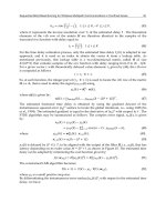
Exercise 1: Verify the approximate attenuation rates in Table 1, Column 3 by using (12) for
the TE
0m
/TM
0m
modes and (15) for the HE
nm
modes.
Exercise 2: Using any root finding software, verify the exact attenuation rates in column 2 of
Table 1. To do so, you need to solve the modal equation (8) for the complex roots of u. You
can use (10),(11) or (13) as initial guess for u of the TE
0m
, TM
0m
and HE
nm
modes
respectively. Once you get u, the complex is obtained from
2 2
a v u
. The mode
attenuation rate
in Neper/m is the negative of the imaginary part of . To convert to
dB/100m, note that 1 Neper/m= 868.8 dB/100m.
3.3 Mode Excitation
In the above we have ordered the modes in ascending order of their attenuation rates.
However, the actual level of the modes at a given distance from the source is determined
also by their excitation factor, which in turn depends on their field distribution and the
source type, location and orientation. The E-field distribution of the TE
01
and the HE
11
modes, which are the least attenuated modes, are sketched in Figure 2. The TE
01
mode has a
circumferential E
field, which vanishes at =0 and is quite weak at the wall =a (being
proportional to J
1
(u/a)). It follows that the TE
01
mode can be excited by a circumferentially
oriented linear dipole. For optimum excitation, the linear dipole should neither be at the
center or very close to the wall. Alternatively, the TE
01
mode can also be excited by a current
loop placed in the cross section plane near the center of the tunnel. This will couple with H
z
which is maximum at the tunnel center. Dudley (2005) has given rigorous treatment of TE
0
modes excitation by a loop, which is located coaxially with the tunnel.
On the other hand, the HE
11
mode is almost linearly polarized as demonstrated in the
Appendix (see equation A6). So, this mode is optimally excited by a linear dipole close to
the center of the tunnel. A detailed rigorous treatment of the HE
nm
mode excitation by a
linear dipole is found in (Dudley and Mahmoud, 2006).
Fig. 2. E-field lines of the lowest order modes in a circular tunnel.
Here we derive a simple formula for the excitation coefficient of the propagating modes in
the tunnel. The source is assumed to be a small linear electric dipole of vector moment
' 'P
(Ampere-m) located at (
) in the cross section at, say z=0 and oriented along an arbitrary
direction in the transverse plane. The total excited fields ( , )E H
are expressed as a sum over
the natural modes in the tunnel, so
( , ) ( , ) exp( )
r r r r
r
E H A e h j z
(17)
Where
( , ) , 1, 2
r r
e h r
are the normal modal fields ordered in an arbitrary manner. The A
r
are the excitation coefficients. The +
signs correspond to the fields in the z>0 and z<0
respectively. To the above sum we should add a continuous of waves representing radiation
TE
01
mode HE
11
mode
MobileandWirelessCommunications:Physicallayerdevelopmentandimplementation8
through the surrounding host medium. However, this is normally heavily attenuated as
demonstrated in (Dudley and Mahmoud, 2006) and hence will be omitted. The mode
excitation coefficients are determined based on the orthogonality among the modes in a
tunnel with constant impedance walls (Mahmoud, 1991, section 3.6) and the field
discontinuity at the source. So we get ((Mahmoud, 1991, section 2.11).
.
ˆ
2 ( x ).
r
r r
r r
S
P e
A A
e h z ds
(18)
where the integration is taken over the tunnel cross section bounded by the walls.
Exercise 3: For each of the linear electric dipoles
shown in Figure 3, what are the important excited
modes? [HE11 for dipoles 1, and 2, Both HE11 and TE01
modes for dipoles 3 and 4].
Exercise 4: Apply (18) to get the excitation coefficient
for the HE11 mode when excited by a unit y-directed
dipole moment;
ˆ
P y
located at the center of the
tunnel
=0. Note that ( , )
t t
e h
are given by equations
(A6-A7) in the Appendix. To simplify the problem,
assume that the frequency is high enough so that
0
1k and
. Find the power
launched in the HE
11
mode.
4. A rectangular tunnel
Modal propagation in rectangular waveguides with imperfectly conducting walls is
considered to be an intractable problem in waveguide theory. In fact, as indicated by (Wait,
1967) long time ago, there is a fundamental difficulty with mode analysis in cylindrical
waveguides with finite impedance walls and cross-sections other than circular. In such
waveguides, a natural mode does not take the form of a wave with a single transverse
wavenumber as is the case with waveguides with perfectly reflecting walls. In contrast, a
waveguide mode is generally composed of a weighted sum of elementary waves having a
single transverse wavenumber each. A comprehensive discussion of this phenomenon is
reviewed by Mahmoud (1991 sec. 3.5) in relation to elliptical and rectangular waveguides.
However, simple, but approximate modal solutions valid in the high frequency regime have
been obtained by several authors. Marcatili &Scmeltzer (1964) obtain the x and y transverse
wavenumber approximately by treating the rectangular waveguide as two parallel plates in
the y and x directions respectively. Andersen et al. (1975) derive an aprproximate modal
equation for the transverse wavenumber by considering the mode to be composed of four
crossing plane waves interconnected at the tunnel walls by reflection matrices. The method
accounts for the coupling between horizontal and vertical polarizations upon reflection.
1
2
3
4
Fi
g
.
3.
Wait [1980] and Mahmoud [1991, sec. 6.2.2] obtain an approximate TM type modal solution
based on the neglect of one weak boundary condition. In the following, we outline this
formulation.
So, consider a rectangular guide of width w and height h and outer medium of complex
relative permittivity
c
(=
r
-i
0
) as depicted in Figure 4. The walls are characterized by
constant impedance and admittance
,
s
s
Z
Y as given by (4). For a TM
y
mode, or a vertically
polarized mode, E
x
=0 and E
y
may be given, for an even mode, by:
cos( )cos( )exp( )
y y x
E k y k x j z
(19)
Fig. 4. A rectangular tunnel in a host medium
In the above:
2 2 2 2
0
y x
k k k
. Because the guide is oversized relative to the wavelength,
both k
x
and k
y
are << k
0
and
for the low order modes. The E
z
component is obtained from
the divergence equation
. 0E
, hence:
/
z y
j
E E y
(20)
which shows that E
z
is of first order smallness relative to E
y
. The magnetic field components
are obtained as:
0 0 0 0 0
/ , 0, /
x y y z y
H E k H and H j E k x
(21)
where terms of second order smallness have been neglected (such as
2
0
/
x y
k k k ). Now the
boundary condition at y=+h/2 requires that:
0
( / ) |
x
z y b s
H E Y
, which reduces to:
r
,
w
h
x
y
WirelessTransmissioninTunnels 9
through the surrounding host medium. However, this is normally heavily attenuated as
demonstrated in (Dudley and Mahmoud, 2006) and hence will be omitted. The mode
excitation coefficients are determined based on the orthogonality among the modes in a
tunnel with constant impedance walls (Mahmoud, 1991, section 3.6) and the field
discontinuity at the source. So we get ((Mahmoud, 1991, section 2.11).
.
ˆ
2 ( x ).
r
r r
r r
S
P e
A A
e h z ds
(18)
where the integration is taken over the tunnel cross section bounded by the walls.
Exercise 3: For each of the linear electric dipoles
shown in Figure 3, what are the important excited
modes? [HE11 for dipoles 1, and 2, Both HE11 and TE01
modes for dipoles 3 and 4].
Exercise 4: Apply (18) to get the excitation coefficient
for the HE11 mode when excited by a unit y-directed
dipole moment;
ˆ
P y
located at the center of the
tunnel
=0. Note that ( , )
t t
e h
are given by equations
(A6-A7) in the Appendix. To simplify the problem,
assume that the frequency is high enough so that
0
1k and
. Find the power
launched in the HE
11
mode.
4. A rectangular tunnel
Modal propagation in rectangular waveguides with imperfectly conducting walls is
considered to be an intractable problem in waveguide theory. In fact, as indicated by (Wait,
1967) long time ago, there is a fundamental difficulty with mode analysis in cylindrical
waveguides with finite impedance walls and cross-sections other than circular. In such
waveguides, a natural mode does not take the form of a wave with a single transverse
wavenumber as is the case with waveguides with perfectly reflecting walls. In contrast, a
waveguide mode is generally composed of a weighted sum of elementary waves having a
single transverse wavenumber each. A comprehensive discussion of this phenomenon is
reviewed by Mahmoud (1991 sec. 3.5) in relation to elliptical and rectangular waveguides.
However, simple, but approximate modal solutions valid in the high frequency regime have
been obtained by several authors. Marcatili &Scmeltzer (1964) obtain the x and y transverse
wavenumber approximately by treating the rectangular waveguide as two parallel plates in
the y and x directions respectively. Andersen et al. (1975) derive an aprproximate modal
equation for the transverse wavenumber by considering the mode to be composed of four
crossing plane waves interconnected at the tunnel walls by reflection matrices. The method
accounts for the coupling between horizontal and vertical polarizations upon reflection.
1
2
3
4
Fi
g
.
3.
Wait [1980] and Mahmoud [1991, sec. 6.2.2] obtain an approximate TM type modal solution
based on the neglect of one weak boundary condition. In the following, we outline this
formulation.
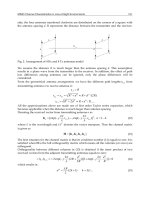
So, consider a rectangular guide of width w and height h and outer medium of complex
relative permittivity
c
(=
r
-i
0
) as depicted in Figure 4. The walls are characterized by
constant impedance and admittance
,
s
s
Z
Y as given by (4). For a TM
y
mode, or a vertically
polarized mode, E
x
=0 and E
y
may be given, for an even mode, by:
cos( )cos( )exp( )
y y x
E k y k x j z
(19)
Fig. 4. A rectangular tunnel in a host medium
In the above:
2 2 2 2
0
y x
k k k
. Because the guide is oversized relative to the wavelength,
both k
x
and k
y
are << k
0
and
for the low order modes. The E
z
component is obtained from
the divergence equation
. 0E
, hence:
/
z y
j
E E y
(20)
which shows that E
z
is of first order smallness relative to E
y
. The magnetic field components
are obtained as:
0 0 0 0 0
/ , 0, /
x y y z y
H E k H and H j E k x
(21)
where terms of second order smallness have been neglected (such as
2
0
/
x y
k k k ). Now the
boundary condition at y=+
h/2 requires that:
0
( / ) |
x
z y b s
H E Y
, which reduces to:
r
,
w
h
x
y
MobileandWirelessCommunications:Physicallayerdevelopmentandimplementation10
0
tan ( / 2) /
y y s
k h k h jk h Y (22)
This is an equation for the y-wavenumber and its solution leads to a set of eigenvalues k
yn
,
n=1,2… Now we consider the side walls at x=+
w/2. The boundary conditions at these two
walls are
0y s z
E Z H
(23)
0 y s z
H Y E
(24)
Using (19) and (21) in (23) leads to a modal equation for k
x
.
0
tan( / 2) /
x
x s
k w k w jk w Z (25)
So (25) is an equation for k
x
whose solution leads to a set of eigenvalues k
xm
. This completes
the modal solution except that we have not satisfied boundary condition (24). Fortunately
however, H
y
is of second order smallness for the lower order modes, hence this boundary
condition can be safely neglected.
Approximate solutions of (22) and (25) for k
yn
and k
xm
in the high frequency regime,
(
0 0
,
s
s
k h Y k w Z ) are:
0
0
[1 2 / ]
[1 2 / ]
yn s
xm s
k h n j Y k h
k w m j Z k w
, (26)
where m and n =1,3…are odd integers for the even modes considered. The corresponding
mode attenuation rate is easily obtained as:
2 2 2 3 2 2 2 3
VPmn 0 0
2 Re( ) / 2 Re( )/
s s
n Y k h m Z k w
Neper/m (27)
The attenuation rate of the corresponding horizontally polarized mode may be obtained
from (27) by exchanging w and h. So:
2 2 2 3 2 2 2 3
0 0
2 Re( ) / 2 Re( ) /
HPmn s s
n Y k w m Z k h
Neper/m (28)
These formulas agree with those derived by Emslie et al (1975). It is worth noting that like
the circular tunnel, the attenuation of the dominant modes is inversely proportional to the
frequency squared and the linear dimensions cubed. Comparing (27) and (28), we infer that
the vertically polarized mode suffers higher attenuation than the horizontally polarized
mode for w>h. Thus, for a rectangular tunnel with w>h, the first horizontally polarized
mode; TM
x11
is the lowest attenuated mode.
Exercise 5: Use (26) to derive (27). In doing so, note that
2 2 2 1/ 2 2 2
0 0
Im[( ) ] (1/ 2 ) Im[ ]
x
m yn xm yn
k k k k k k
. This, of course, is valid only for low order
modes such that
0
/ w and / are <<m n h k
. Compute the attenuation rate of the TM
y11
and
TM
x11
modes in a tunnel having w=2h=4.3 meters at 1 GHz. Take
r
=10 and =0. [13.27 and
2.95 dB/100m]
We can infer from the above discussion that the attenuation caused by the walls which are
perpendicular to the major electric field is much higher than that contributed by the walls
parallel to the electric field.
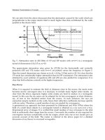
Fig. 5. Attenuation rates in dB/100m of VP and HP modes with m=n=1 in a rectangular
tunnel of dimensions 4.3x2.15 m.
r
=10.
The approximate attenuation rates given by (27-28) for the horizontally and vertically
polarized (HP and VP) modes with m=n=1 are plotted versus the frequency in Figure 5.
Here the tunnel dimensions are chosen as (w,h) = (4.3m, 2.15m) and
r
=10. It is clear that the
VP mode has considerably higher attenuation than its HP counterpart. The attenuation rates
obtained by exact solution of equations (22) and (25) are also plotted for comparison. It is
clear that both solutions coincide at the higher frequencies.
Ray theory:
When it is required to estimate the field at distances close to the source, the mode series
becomes slowly convergent since it is necessary to include many higher order modes. As
clear from the above argument, higher order modes are hard to analyze in a rectangular
tunnel. In this case the ray series can be adopted for its fast convergence at short distances,
say, of tens to few hundred meters from the source. At such distances, the rays are
somewhat steeply incident on the walls, hence their reflection coefficients decrease quickly
with ray order. Therefore, a small number of rays are needed for convergence.
A geometrical ray approach has been presented by (Mahmoud and Wait 1974a) where the
field of a small linear dipole in a rectangular tunnel is obtained as a ray sum over a two-
dimensional array of images. It is verified that small number of rays converges to the total
field at sufficiently short range from the source. Conversely the number of rays required for
convergence increase considerably in the far ranges, where only one or two modes give an
accurate account of the field. The reader is referred to the above paper for a detailed
discussion of ray theory in oversized waveguides.
0
10
20
30
40
50
60
0 400 800 1200 1600 2000
dB/100m
Frequency MHz
Horizontal
Vertical
Solid Curves: Exact
Dashed curves: Approximate