Báo cáo sinh học: " Research Article A Gaussian Mixture Approach to Blind Equalization of Block-Oriented Wireless Communications Frederic Lehmann (EURASIP Member)" doc
Bạn đang xem bản rút gọn của tài liệu. Xem và tải ngay bản đầy đủ của tài liệu tại đây (754.58 KB, 10 trang )
Hindawi Publishing Corporation
EURASIP Journal on Advances in Signal Processing
Volume 2010, Article ID 340417, 10 pages
doi:10.1155/2010/340417
Research Article
A Gaussian Mixture Approach to Blind Equalization of
Block-Oriented Wireless Communications
Frederic Lehmann (EURASIP Member)
Institut TELECOM, TELECOM SudParis, Department CITI, UMR-CNRS 5157, 91011 Evry Cedex, France
Correspondence should be addressed to Frederic Lehmann,
Received 6 October 2009; Revised 12 May 2010; Accepted 30 June 2010
Academic Editor: Tim Davidson
Copyright © 2010 Frederic Lehmann. This is an open access article distributed under the Creative Commons Attribution License,
which permits unrestricted use, distribution, and reproduction in any medium, provided the original work is properly cited.
We consider blind equalization for block transmissions over the frequency selective Rayleigh fading channel. In the absence of pilot
symbols, the receiver must be able to perform joint equalization and blind channel identification. Relying on a mixed discrete-
continuous state-space representation of the communication system, we introduce a blind Bayesian equalization algorithm based
on a Gaussian mixture parameterization of the a posteriori probability density function (pdf) of the transmitted data and the
channel. The performances of the proposed algorithm are compared with existing blind equalization techniques using numerical
simulations for quasi-static and time-varying frequency selective wireless channels.
1. Introduction
Blind equalization has attracted considerable attention in the
communication literature over the last three decades. The
main advantage of blind transmissions is that they avoid
the need for the transmission of training symbols and hence
leave more communication resources for data.
The pioneering blind equalizers proposed by Sato [1]
and Godard [2] use low-complexity finite impulse response
filters. However, these methods suffer from local and slow
convergence and may fail on ill-conditioned or time-varying
channels.
Other authors have proposed symbol-by-symbol soft-
input soft-output (SISO) equalizers based on trellis search
algorithms. Two such approaches have been proposed so
far to achieve SISO equalization in a blind or semiblind
context. The first approach relies on fixed lag smoothing
[3] and was further simplified in [4] by allowing pruning
and decision feedback techniques. The second approach
uses fixed interval smoothing [5, 6]. The aforementioned
methods employ a trellis description of the intersymbol
interference (ISI) [7], where each discrete ISI state has its
associated channel estimate. Another fixed interval method,
based on expectation-maximization channel identification,
has appeared recently [8], but this technique is restricted to
static channels.
In this paper, we will consider fixed interval smoothing,
which is adapted to block-oriented communications. After
modeling the ISI and the unknown channel at the receiver
side, we obtain a combined state-space formulation of our
communication system. Specifically, the ISI is modeled as
a discrete state space with memory, while the (potentially
time-varying) channel is modeled as an autoregressive (AR)
process.
Main Contributions and Related Work. The main technical
contribution of this work is the introduction of a blind
equalization technique based on Gaussian mixtures. A major
problem in blind equalization is that multiple modes arise
in the a posteriori channel pdf, which originate from the
phase ambiguities inherent to digital modulations. Assume
that an equalizer is able to represent only a single mode,
as is usually the case, it is likely that the wrong mode is
retained during a fading event or due to the occasional
occurrence of high observation noise. In such a situation,
a classical equalizer is not able to recover the correct phase
determination in a blind mode, since no pilot symbol is
available. Therefore, all the subsequent decisions in the frame
will be erroneous with high probability. The main feature
of the proposed algorithm is that the multimodality of the
channel a posteriori pdf is explicitly taken into account
thanks to a Gaussian mixture parameterization. We derive
2 EURASIP Journal on Advances in Signal Processing
Information bits Tail
B bits
Figure 1: Data format.
{c
i
k
}
L
i
=0
y
k
Channel
b
k
n
k
Figure 2: Channel model.
the corresponding SISO smoothing algorithm suitable to
solve our blind equalization problem.
Note that the idea of Gaussian mixture processing has
been presented in [9] in the context of MIMO decoding and
that the results in this paper have been partially presented in
[10]. Also the idea of exploiting Gaussian mixtures for blind
equalization appeared previously in a different form [11].
Organization. Section 2 describes the adopted system mod-
el. Section 3 introduces the Gaussian mixture-based blind
equalization technique. Finally, in Section 4, the performa-
nces of the proposed technique are assessed through
numerical simulations and compared with existing blind
equalization techniques.
Notations. Throughout the paper, bold letters indicate vec-
tors and matrices. N
C
(x : m, P) will denote a complex
Gaussian distribution of the variable x,withmeanm and
covariance matrix P. I
m
denotes the m × m identity matrix,
while 0
m
denotes the m × m all-zero matrix. The symbol
⊗ denotes the Kronecker product. The operator det(·)will
denote the determinant of a matrix.
2. System Model
The transmitted data are organized in GSM-like bursts
containing B bits, as illustrated in Figure 1. For ease of
exposition, we consider binary phase shift keying (BPSK)
modulation, so that the bit is transmitted at instant k, b
k
∈
{−
1, +1}. The tail is a short all-one vector of length equal
to the channel memory, used to set the final ISI state of the
current data burst to a known value. At the same time, this
also sets the initial ISI state of the next data burst to the
same known value. Since blind equalization is of interest, no
additional pilot symbols are inserted in the data stream.
We assume a discrete Rayleigh fading channel of memory
L as depicted in Figure 2. The elements of the impulse
response
{c
i
k
}
L
i
=0
are modeled as independent zero-mean
complex Gaussian random variables. For a static channel, the
channel state is defined as x
k
= [c
0
k
, c
1
k
, , c
L
k
]
T
and evolves
according to the trivial dynamical system
x
k
= x
k−1
.
(1)
For a time-varying channel, let B
d
and T denote the max-
imum Doppler shift and the symbol duration, respectively.
Thechannelautocorrelationcanbemodeledasfollows[12]:
E
c
i
k
c
i
k
−n
∗
=
J
0
(
2πnB
d
T
)
, i = 0, , L,(2)
where J
0
is the zero-order Bessel function of first kind. A
good approximation of the channel statistics is obtained with
an order two autoregressive process [13] of the following
form:
c
i
k
= φ
1
c
i
k
−1
+ φ
2
c
i
k
−2
+ π
i
k
, i = 0, , L,
(3)
by letting
φ
1
= 2r cos
(
ω
)
, φ
2
=−r
2
,
(4)
where r
= 0.809
2πB
d
T
and ω = 0.781 × 2πB
d
T. The driving
noise term π
i
k
is chosen as a zero-mean white complex
Gaussian process of variance
q
=
1+φ
2
1 − φ
2
1 − φ
2
2
− φ
2
1
,
(5)
so as to normalize the channel coefficients to unit vari-
ance [14]. Consequently, the channel state, in the case
of a time-varying wireless channel, is defined as x
k
=
[c
0
k
, c
0
k
−1
, c
1
k
, c
1
k
−1
, , c
L
k
, c
L
k
−1
]
T
and evolves according to the
dynamical system
x
k
= Fx
k−1
+ π
k
,
(6)
where state transition matrix is given by
F
=
⎡
⎢
⎢
⎢
⎢
⎣
Φ 0
2
0
2
0
2
Φ 0
2
.
.
.
.
.
.
.
.
.
.
.
.
0
2
0
2
Φ
⎤
⎥
⎥
⎥
⎥
⎦
, Φ =
φ
1
φ
2
10
,(7)
and the process noise vector is given by
π
k
=
π
0
k
,0,π
1
k
,0, , π
L
k
,0
T
.
(8)
The received complex noisy observation at instant k has
the following form:
y
k
=
L
i=0
c
i
k
b
k−i
+ n
k
,
(9)
where n
k
is a complex white Gaussian noise sample with
single-sided power spectral density N
0
.
We define the ISI state s
k
as the decimal form of the
binary subsequence [b
k
, b
k−1
, , b
k−L+1
]
T
,whichcantake2
L
EURASIP Journal on Advances in Signal Processing 3
discrete values. Let f
k
denote the ISI state transition function
defined by the following relation:
s
k
= f
k
(
s
k−1
, b
k
)
.
(10)
It is well known that f
k
can be represented graphically by a
trellis diagram containing 2
L
states [7].
For a time-varying channel, it is now clear from (6)and
(9) that our communication system can be described as a
mixed discrete-continuous state space of the form (s
k
, x
k
),
whose dynamics are given by
s
k
= f
k
(
s
k−1
, b
k
)
,
x
k
= Fx
k−1
+ π
k
,
y
k
= h
k
(
s
k−1
, s
k
)
T
x
k
+ n
k
.
(11)
Thesecondequationin(11) can be interpreted as a linear
dynamical system with state transition matrix given by (7)
and zero-mean Gaussian process noise, with covariance
matrix
Q
= qI
L+1
⊗
10
00
. (12)
The third equation in (11) can be interpreted as a lin-
ear observation process, where the observation matrix
h
k
(s
k−1
, s
k
) has the form
h
k
(
s
k−1
, s
k
)
=
[
b
k
,0,b
k−1
,0, , b
k−L
,0
]
T
.
(13)
From (1)and(9), a slightly different state-space repre-
sentation is obtained for the static channel as a special case of
(11) by choosing F
= I
L+1
, Q = O
L+1
,and
h
k
(
s
k−1
, s
k
)
=
[
b
k
, b
k−1
, , b
k−L
]
T
.
(14)
3. Blind SISO Equalization Using a Gaussian
Mixture Approach
In this section, we derive a fixed-interval smoother by
propagating a mixture of N Gaussians per ISI state forward
and backward in the ISI trellis. Consequently, the ISI state s
k
and the channel state x
k
will be jointly estimated. Finally, the
desired a posteriori probabilities for the bits b
k
are obtained
by a simple marginalization step.
3.1. Forward Filtering. A recursive expression of p(s
k
, x
k
|
y
1:k
), where y
1:k
= (y
1
, y
2
, , y
k
) is obtained by noting that
p
s
k
, x
k
, y
1:k
=
s
k−1
p
(
s
k
| s
k−1
)
p
y
k
| h
k
(
s
k−1
, s
k
)
, x
k
×
p
(
x
k
| x
k−1
)
p
s
k−1
, x
k−1
, y
1:k−1
dx
k−1
,
(15)
where the discrete summation extends over the states s
k−1
,
for which a valid transition (s
k−1
, s
k
) exists. In general, the
multiplications and integration in (15) cannot be expressed
in closed form, therefore, we introduce the following Gaus-
sian mixture parameterization at instant k
− 1:
p
s
k−1
, x
k−1
, y
1:k−1
=
N
i=1
α
i
(
s
k−1
)
N
C
x
k−1
: x
i
k
−1|k−1
(
s
k−1
)
, P
i
k
−1|k−1
(
s
k−1
)
.
(16)
In (16), each discrete state s
k−1
is associated with a mixture
of N Gaussians, where N is a design parameter of choice.
Theorem 1. A closed form expression of p(s
k
, x
k
, y
1:k
) is
obtained as follows:
p
s
k
, x
k
, y
1:k
=
s
k−1
N
i=1
α
i
(
s
k−1
, s
k
)
N
C
x
k
: x
i
k
|k
(
s
k−1
, s
k
)
, P
i
k
|k
(
s
k−1
, s
k
)
,
(17)
where the means x
i
k
|k
(s
k−1
, s
k
) and covariance matrices
P
i
k
|k
(s
k−1
, s
k
) associated with the state transition (s
k−1
, s
k
) are
obtained from the following recursions:
x
i
k
|k−1
(
s
k−1
)
= Fx
i
k
−1|k−1
(
s
k−1
)
,
P
i
k
|k−1
(
s
k−1
)
= FP
i
k
−1|k−1
(
s
k−1
)
F
H
+ Q,
K
i
k
(
s
k−1
, s
k
)
= P
i
k
|k−1
(
s
k−1
)
h
k
(
s
k−1
, s
k
)
∗
×
h
k
(
s
k−1
, s
k
)
T
P
i
k
|k−1
(
s
k−1
)
h
k
(
s
k−1
, s
k
)
∗
+N
0
−1
,
x
i
k
|k
(
s
k−1
, s
k
)
= x
i
k
|k−1
(
s
k−1
)
+ K
i
k
(
s
k−1
, s
k
)
×
y
k
− h
k
(
s
k−1
, s
k
)
T
x
i
k
|k−1
(
s
k−1
)
,
P
i
k
|k
(
s
k−1
, s
k
)
= P
i
k
|k−1
(
s
k−1
)
− K
i
k
(
s
k−1
, s
k
)
h
k
(
s
k−1
, s
k
)
T
× P
i
k
|k−1
(
s
k−1
)
,
(18)
and the weights α
i
(s
k−1
, s
k
) are given by
α
i
(
s
k−1
, s
k
)
= α
i
(
s
k−1
)
p
(
s
k
| s
k−1
)
× N
C
yk : h
k
(
s
k−1
, s
k
)
T
x
i
k
|k−1
(
s
k−1
)
,
h
k
(
s
k−1
, s
k
)
T
P
i
k
|k−1
(
s
k−1
)
×h
k
(
s
k−1
, s
k
)
∗
+ N
0
.
(19)
4 EURASIP Journal on Advances in Signal Processing
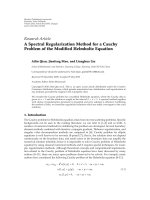
p(s
k−1
= 2, x
k−1
, y
1:k−1
)
p(s
k−1
= 0, x
k−1
, y
1:k−1
) p(s
k
= 0, x
k
, y
1:k
)
Figure 3: Example of forward propagation of Gaussian mixtures
(with N
= 4) on a 4-state trellis.
Proof. Injecting (16) into (15), one obtains
p
s
k
, x
k
, y
1:k
=
s
k−1
N
i=1
α
i
(
s
k−1
)
p
(
s
k
| s
k−1
)
p
y
k
| h
k
(
s
k−1
, s
k
)
, x
k
×
p
(
x
k
| x
k−1
)
× N
C
x
k−1
: x
i
k
−1|k−1
(
s
k−1
)
, P
i
k
−1|k−1
(
s
k−1
)
dx
k−1
.
(20)
In the above expression, we easily recognize the integral as
the well-known prediction step of Kalman filtering [14].
Moreover, the multiplication by p(y
k
| h
k
(s
k−1
, s
k
), x
k
) is the
correction step of Kalman filtering. Therefore, p(s
k
, x
k
, y
1:k
)
can be written as (17).
Figure 3 illustrates how the Gaussian mixture p(s
k
=
0, x
k
, y
1:k
) is computed on a 4-state trellis. The components
of the Gaussian mixtures p(s
k−1
= 0, x
k−1
, y
1:k−1
)and
p(s
k−1
= 2, x
k−1
, y
1:k−1
) undergo a Kalman prediction and
correction given the hypothesized data symbol on the valid
trellis branch (s
k−1
= 0,s
k
= 0) and (s
k−1
= 2,s
k
=
0), respectively. The resulting Gaussian mixture p(s
k
=
0, x
k
, y
1:k
) is obtained as a weighted sum of the resulting
mixtures.
3.2. Complexity Reduction Algorithm (CRA). Aproblemwith
(17) is that each discrete state s
k
is now associated with
a mixture of more than N Gaussians. This means that
the number of terms in the Gaussian mixture will grow
with time. In order to keep the computational complexity
constant for each time instant, we need to approximate the
exact expression given by (17) as follows:
p
s
k
, x
k
, y
1:k
≈
N
i=1
α
i
(
s
k
)
N
C
x
k
: x
i
k
|k
(
s
k
)
, P
i
k
|k
(
s
k
)
,
(21)
so that again N Gaussianswithweightα
i
(s
k
), mean x
i
k
|k
(s
k
),
and covariance P
i
k
|k
(s
k
), i = 1, , N are associated with each
state s
k
,asin(16). We do this by applying the CRA proposed
in [15]. Assume that N
1
(resp. N
2
) is a multivariate Gaussian,
whose weight, mean, and covariance are given by w
1
, x
1
,and
P
1
(resp. w
2
, x
2
, P
2
). In [15], a practical measure of similarity
between the two densities is given by
D
= w
1
w
2
[
I
(
N
1
N
2
)
+ I
(
N
2
N
1
)
]
,
(22)
where I(
··) denotes the Kullback-Leibler distance. Then,
pairs of similar Gaussians with minimal D are repeatedly
merged until N Gaussians remain using the following
approximation:
w
1
N
C
(
x
k
: x
1
, P
1
)
+ w
2
N
C
(
x
k
: x
2
, P
2
)
≈ wN
C
(
x
k
: x, P
)
,
(23)
where
w
= w
1
+ w
2
,
x
=
w
1
x
1
+ w
2
x
2
w
1
+ w
2
,
P
=
w
1
w
1
+ w
2
P
1
+
(
x
1
− x
)(
x
1
− x
)
H
+
w
2
w
1
+ w
2
P
2
+
(
x
2
− x
)(
x
2
− x
)
H
.
(24)
3.3. Backward Filtering. Let T denote the total number of
available observations and y
k+1:T
= (y
k+1
, y
k+2
, , y
T
). A
time-reversed version of the forward filter in Section 3.1
can also be derived. We seek a recursive expression of the
likelihood p(y
k+1:T
| s
k
, x
k
), propagated backward in time.
We obtain the following recursion:
p
y
k+1:T
| s
k
, x
k
=
s
k+1
p
(
s
k+1
| s
k
)
×
p
(
x
k+1
| x
k
)
× p
y
k+1
| h
k+1
(
s
k
, s
k+1
)
, x
k+1
×
p
y
k+2:T
| s
k+1
, x
k+1
dx
k+1
,
(25)
where the discrete summation extends over the states s
k+1
,for
which a valid transition (s
k
, s
k+1
) exists.
Theorem 2. Assume that the following Gaussian mixture
parameterization:
p
y
k+2:T
| s
k+1
, x
k+1
=
N
i=1
β
i
(
s
k+1
)
N
C
x
k+1
: x
i
k+1
|k+2:T
(
s
k+1
)
, P
i
k+1
|k+2:T
(
s
k+1
)
(26)
EURASIP Journal on Advances in Signal Processing 5
is available at instant k +1, a closed for m ex pression of
p(y
k+1:T
s
k
, x
k
) is obtained as
p
y
k+1:T
| s
k
, x
k
=
s
k+1
N
i=1
β
i
(
s
k
, s
k+1
)
N
C
x
k
: x
i
k
|k+1:T
(
s
k
, s
k+1
)
,
P
i
k
|k+1:T
(
s
k
, s
k+1
)
,
(27)
where the means x
i
k
|k+1:T
(s
k
, s
k+1
) and covariance matrices
P
i
k
|k+1:T
(s
k
, s
k+1
) associated with the state t ransition (s
k
, s
k+1
)
areobtainedfromthefollowingrecursions:
K
i
k+1
(
s
k
, s
k+1
)
= P
i
k+1
|k+2:T
(
s
k+1
)
h
k+1
(
s
k
, s
k+1
)
∗
×
h
k+1
(
s
k
, s
k+1
)
T
P
i
k+1
|k+2:T
(
s
k+1
)
h
k+1
(
s
k
, s
k+1
)
∗
+N
0
−1
,
x
i
k+1
|k+1:T
(
s
k
, s
k+1
)
= x
i
k+1
|k+2:T
(
s
k+1
)
+ K
i
k+1
(
s
k
, s
k+1
)
×
y
k+1
− h
k+1
(
s
k
, s
k+1
)
T
x
i
k+1
|k+2:T
(
s
k+1
)
,
P
i
k+1
|k+1:T
(
s
k
, s
k+1
)
= P
i
k+1
|k+2:T
(
s
k+1
)
− K
i
k+1
(
s
k
, s
k+1
)
× h
k+1
(
s
k
, s
k+1
)
T
P
i
k+1
|k+2:T
(
s
k+1
)
,
x
i
k
|k+1:T
(
s
k
, s
k+1
)
= Fx
i
k+1
|k+1:T
(
s
k
, s
k+1
)
,
P
i
k
|k+1:T
(
s
k
, s
k+1
)
= FP
i
k+1
|k+1:T
(
s
k
, s
k+1
)
F
H
+ Q,
(28)
and the weights β
i
(s
k
, s
k+1
) are given by
β
i
(
s
k
, s
k+1
)
= β
i
(
s
k+1
)
p
(
s
k+1
| s
k
)
×N
C
y
k+1
: h
k+1
(
s
k
, s
k+1
)
T
x
i
k+1
|k+2:T
(
s
k+1
)
,
h
k+1
(
s
k
, s
k+1
)
T
P
i
k+1
|k+2:T
(
s
k+1
)
h
k+1
(
s
k
, s
k+1
)
∗
+N
0
.
(29)
The proof is obtained by injecting (26) into (25) and using the
same arguments as in the demonstration of Theorem 1.
Figure 4 illustrates how the Gaussian mixture p(y
k+1:T
|
s
k
= 1,x
k
) is computed on a 4-state trellis. The components
of the Gaussian mixtures p(y
k+2:T
| s
k+1
= 2,x
k+1
)and
p(y
k+2:T
| s
k+1
= 3, x
k+1
)undergoaKalmancorrection
and backward prediction given the hypothesized data symbol
on the valid trellis branch (s
k
= 1, s
k+1
= 2) and (s
k
=
1, s
k+1
= 3), respectively. The resulting Gaussian mixture
p(y
k+1:T
| s
k
= 1, x
k
) is obtained as a weighted sum of the
resulting mixtures.
p(y
k+2:T
|s
k+1
= 3, x
k+1
)
p(y
k+2:T
|s
k+1
= 2, x
k+1
)
p(y
k+1:T
|, s
k
= 1, x
k
)
Figure 4: Example of backward propagation of Gaussian mixtures
(with N
= 4) on a 4-state trellis.
Again, we need to apply the CRA of Section 3.2.Com-
plexity reduction algorithm to (27), so that p(y
k+1:T
| s
k
, x
k
)
admits the desired form
p
y
k+1:T
| s
k
, x
k
≈
N
i=1
β
i
(
s
k
)
N
C
x
k
: x
i
k
|k+1:T
(
s
k
)
, P
i
k
|k+1:T
(
s
k
)
.
(30)
3.4. Smoothing. A two-filter smoothing formula is obtained
as follows:
p
s
k
, s
k+1
, x
k
, y
1:T
=
p
(
s
k+1
| s
k
)
p
s
k
, x
k
, y
1:k
×
p
(
x
k+1
| x
k
)
p
y
k+1
| h
k+1
(
s
k
, s
k+1
)
, x
k+1
×
p
y
k+2:T
| s
k+1
, x
k+1
dx
k+1
.
(31)
Theorem 3. Using the Gaussian mixture approximations
for the forward and the backward filter introduced in Sec-
tions 3.1 and 3.3, respectively, a closed form expression of
p(s
k
, s
k+1
, x
k
, y
1:T
) is obtained as follows:
p
s
k
, s
k+1
, x
k
, y
1:T
=
N
i=1
N
j=1
σ
i,j
(
s
k
, s
k+1
)
N
C
x
k
: x
i,j
k
|1:T
(
s
k
, s
k+1
)
, P
i,j
k
|1:T
(
s
k
, s
k+1
)
,
(32)
where the covariances associated to transition (s
k
, s
k+1
) are
P
i,j
k
|1:T
(
s
k
, s
k+1
)
= P
j
k
|k+1:T
(
s
k
, s
k+1
)
×
P
j
k
|k+1:T
(
s
k
, s
k+1
)
+ P
i
k
|k
(
s
k
)
−1
× P
i
k
|k
(
s
k
)
,
(33)
6 EURASIP Journal on Advances in Signal Processing
and the means associated to transition (s
k
, s
k+1
) are
x
i,j
k
|1:T
(
s
k
, s
k+1
)
= P
i,j
k
|1:T
(
s
k
, s
k+1
)
×
P
i
k
|k
(
s
k
)
−1
x
i
k
|k
(
s
k
)
+ P
j
k
|k+1:T
(
s
k
, s
k+1
)
−1
× x
j
k
|k+1:T
(
s
k
, s
k+1
)
,
(34)
for 1
≤ i, j ≤ N. The expression of the we ights is given by
σ
i,j
(
s
k
, s
k+1
)
= α
i
(
s
k
)
β
j
(
s
k+1
)
p
(
s
k+1
| s
k
)
b
i,j
(
s
k
, s
k+1
)
× N
C
y
k+1
: h
k+1
(
s
k
, s
k+1
)
T
x
j
k+1
|k+2:T
(
s
k+1
)
,
h
k+1
(
s
k
, s
k+1
)
T
P
j
k+1
|k+2:T
(
s
k+1
)
h
k+1
(
s
k
, s
k+1
)
∗
+N
0
.
(35)
The coefficient b
i,j
(s
k
, s
k+1
) has the following form:
b
i,j
(
s
k
, s
k+1
)
=
1
π
d
det
P
j
k
|k+1:T
(
s
k
, s
k+1
)
+ P
i
k
|k
(
s
k
)
×
exp
−
x
i
k
|k
(s
k
) − x
j
k
|k+1:T
(s
k
, s
k+1
)
H
P
j
k
|k+1:T
(
s
k
, s
k+1
)
+ P
i
k
|k
(
s
k
)
−1
x
i
k
|k
(
s
k
)
− x
j
k
|k+1:T
(
s
k
, s
k+1
)
,
(36)
where d denotes the dimension of the continuous valued state
variable.
Proof. In (31), the term p(s
k
, x
k
, y
1:k
) has been calculated as
(21) and the integral, also appearing in (25), has already been
computed as
N
j=1
β
j
(
s
k+1
)
× N
C
y
k+1
: h
k+1
(
s
k
, s
k+1
)
T
x
j
k+1
|k+2:T
(
s
k+1
)
,
h
k+1
(
s
k
, s
k+1
)
T
P
j
k+1
|k+2:T
(
s
k+1
)
h
k+1
(
s
k
, s
k+1
)
∗
+N
0
×
N
C
x
k
: x
j
k
|k+1:T
(
s
k
, s
k+1
)
, P
j
k
|k+1:T
(
s
k
, s
k+1
)
.
(37)
p(y
k+2:T
|s
k+1
= 3, x
k+1
)
p(s
k
= 1, x
k
, y
1:k
)
Figure 5: Illustration of the computation of smoothed Gaussian
mixtures (with N
= 4) on a 4-state trellis.
Therefore, (31) can be rewritten as follows:
N
i=1
N
j=1
α
i
(
s
k
)
β
j
(
s
k+1
)
p
(
s
k+1
| s
k
)
×N
C
y
k+1
: h
k+1
(
s
k
, s
k+1
)
T
x
j
k+1
|k+2:T
(
s
k+1
)
,
h
k+1
(
s
k
, s
k+1
)
T
P
j
k+1
|k+2:T
(
s
k+1
)
h
k+1
(
s
k
, s
k+1
)
∗
+N
0
×
N
C
x
k
: x
i
k
|k
(
s
k
)
, P
i
k
|k
(
s
k
)
×
N
C
x
k
: x
j
k
|k+1:T
(
s
k
, s
k+1
)
, P
j
k
|k+1:T
(
s
k
, s
k+1
)
.
(38)
After straightforward algebraic manipulations on the prod-
uct of two Gaussian densities, the desired result (32)is
obtained.
Figure 5 illustrates how the Gaussian mixture p(s
k
=
1, s
k+1
= 3, x
k
, y
1:T
) is computed on a 4-state trellis. The com-
ponents of the Gaussian mixtures p(y
k+2:T
| s
k+1
= 3,x
k+1
)
undergo a Kalman correction and backward prediction given
the hypothesized data symbol on the valid trellis branch (s
k
=
1, s
k+1
= 3). The resulting Gaussian mixture is multiplied
with the Gaussian mixture p(s
k
= 1, x
k
, y
1:k
)computedin
the forward pass and by the scalar p(s
k+1
= 3 | s
k
= 1), so as
to obtain p(s
k
= 1, s
k+1
= 3, x
k
, y
1:T
).
Since we are interested in soft-output equalization, we
must compute smoothed bit-by-bit marginal probabilities.
Let B
(m)
k
be the set of state transitions (s
k−1
, s
k
) such that the
information bit b
k
= m,withm =−1,1. Taking (32)at
instant k
−1 and marginalizing out the vector x
k−1
,weobtain
p
b
k
= m | y
1:T
∝
(s
k−1
,s
k
)∈B
(m)
k
N
i=1
N
j=1
σ
i,j
(
s
k−1
, s
k
)
.
(39)
The hard decision can then be written as follows:
b
k
= arg max
m∈{−1,+1}
p
b
k
= m | y
1:T
.
(40)
EURASIP Journal on Advances in Signal Processing 7
Similarly, the a posteriori pdf of the channel vector is
obtained as a Gaussian mixture by marginalizing out all
possible ISI state transitions
p
x
k
| y
1:T
∝
(s
k
,s
k+1
)
N
i=1
N
j=1
σ
i,j
(
s
k
, s
k+1
)
× N
C
x
k
: x
i,j
k
|1:T
(
s
k
, s
k+1
)
, P
i,j
k
|1:T
(
s
k
, s
k+1
)
.
(41)
Under the minimum mean square error (MMSE) crite-
rion, the forward filtered channel vector estimated at instant
k is obtained by marginalizing out the ISI state variable
x
k|k
=
x
k
p
x
k
| y
1:k
dx
k
∝
s
k
N
i=1
α
i
(
s
k
)
x
i
k
|k
(
s
k
)
. (42)
Similarly, the MMSE smoothed estimate of the channel
vector at instant k is obtained by marginalizing out all
possible ISI state transitions
x
k|1:T
=
x
k
p
x
k
| y
1:T
dx
k
∝
(s
k
,s
k+1
)
N
i=1
N
j=1
σ
i,j
(
s
k
, s
k+1
)
x
i,j
k
|1:T
(
s
k
, s
k+1
)
.
(43)
3.5. Complexity Evaluation. It is well known that the com-
plexity of one recursion of the Kalman filter is O(d
3
)[16],
where d denotes the dimension of the continuous-valued
state estimate. However, in our forward and backward filters,
the complexity of one recursion of the Kalman filter reduces
to O(d
2
) due to the block diagonal form of F and the fact that
the matrix inversion reduces to a division by a scalar. Thus,
the overall complexity per information bit of the forward
and backward filter is O(2
L
(L +1)
2
N). The complexity per
information bit of the smoothing pass can be evaluated as
O(2
L
(L +1)
3
N
2
), due to the matrix inversions.
4. Numerical Results
4.1. Comparis on with Existing Methods. We consider a
memory-2 Rayleigh fading channel simulated with the
method introduced in [17]. The standard deviations of
the resulting three complex processes (c
0
k
, c
1
k
, c
2
k
) are set at
(0.407, 0.815, 0.407). The block size is B
= 100 bits. As
illustrated in Figure 1, a tail of length 2 bits is used, which
enables the proposed algorithm to start with the correct
initial and final ISI state when processing each frame. This
is necessary to remove the
±π phase ambiguity inherent
to BPSK modulation. We assume that each data block is
affected by an independent channel realization. E
b
denotes
the average energy per bit.
We compare the bit error rate (BER) of our method
with two kinds of blind equalizers. The first kind of blind
equalizers consists of Baud-rate linear filters optimized with
the constant modulus algorithm (CMA) [2] or with the first
cost function (FCF) introduced in [18]. These equalizers
10
−4
10
−3
10
−2
10
−1
10
0
BER
0 5 10 15 20 25 30 35 40 45
E
b
/N
0
(dB)
PSP
FCF
CMA
Gaussian mixture smoother -N
= 1
Gaussian mixture smoother -N
= 2
Perfect CSI
Figure 6: BER performances of blind equalization at B
d
T = 0.
are iterated 50 times back and forth on each data block, in
order to aleviate the slow convergence problem [19]. There
is also the issue of the ambiguities inherent to these blind
equalizers. Differential encoding of the transmitted data is
used to solve the phase ambiguity problem. Also, a length-
10 known preamble is used to resolve the delay ambiguity.
The lengths of the CMA and FCF equalizers were optimized
by hand, to 5 and 15 coefficients, respectively. The second
kind of blind equalizer is the per-survivor processing (PSP)
algorithm [20], which is similar in spirit to the proposed
method, since it is a trellis-based algorithm operating on the
conventional 4-state ISI trellis [7] and using Kalman filtering
for channel estimation. However, since the path pruning
strategy employs the Viterbi algorithm [7], it is not an SISO
method.
Figure 6 illustrates the BER of the different equalizers
as a function of E
b
/N
0
for a static Rayleigh fading channel
(B
d
T = 0). The CMA and FCF equalizers reach an error
floor due to residual ISI. The same phenonenon is observed
for the PSP algorithm and is due to the misacquisition
problem analysed in [21]. Our Gaussian mixture smoother
in the degenerate case, where the channel estimation is
performed with only N
= 1 Gaussian per discrete ISI state,
is clearly outperformed by the proposed algorithm with
N
= 2, which attains performances close to perfect channel
state information (CSI). Note that our Gaussian mixture
smoother with N
= 1 is essentially the same as [3], but
adapted to block transmissions, since fixed-lag smoothing
has been replaced by fixed-interval smoothing.
Figure 7 illustrates the channel mean square error (MSE).
The forward filtered and the smoothed channel estimates
are computed according to (42)and(43), respectively. We
note that smoothing provides a dramatic improvement over
8 EURASIP Journal on Advances in Signal Processing
10
−3
10
−2
10
−1
10
0
MSE
0 5 10 15 20 25 30 35 40 45
E
b
/N
0
(dB)
Forward filter -N
= 1
Smoother -N
= 1
Forward filter -N
= 2
Smoother -N
= 2
Genie-aided
Figure 7: Channel MSE of blind Gaussian mixture-based equaliza-
tion at B
d
T = 0.
10
−4
10
−3
10
−2
10
−1
10
0
BER
0 5 10 15 20 25 30 35 40 45
E
b
/N
0
(dB)
PSP
FCF
CMA
Gaussian mixture smoother -N
= 1
Gaussian mixture smoother -N
= 2
Perfect CSI
Figure 8: BER performances of blind equalization at B
d
T = 10
−2
.
forward filtering alone both for N = 1andN = 2. We
interpret this result by the fact that the smoothing pass, by
exploiting the knowledge of future observations, is able to
correct errors and phase ambiguities due to fading events or
occasionally high noise in the forward pass. As a reference,
the channel MSE attained by a genie-aided Kalman smoother
(with known symbols) is also shown.
We also study a fast-fading scenario with B
d
T = 10
−2
,
in order to study the robustness of our algorithm against
10
−2
10
−1
10
0
MSE
5101520253035
E
b
/N
0
(dB)
Forward filter -N
= 1
Smoother -N
= 1
Forward filter -N
= 2
Smoother -N
= 2
Genie-aided
Figure 9: Channel MSE of blind Gaussian mixture-based equaliza-
tion at B
d
T = 10
−2
.
Table 1: Saleh-Valenzuela model parameters.
Parameter and units Notation and numerical value
Intercluster arrival rate (1/s) Λ = 5/T
Intercluster decay constant (s) Γ
= 0.6T
Intracluster arrival rate (1/s) λ
= 80/T
Intracluster decay constant (s) γ
= 0.35T
a large Doppler spread. Figures 8 and 9 illustrate the BER
and the channel MSE, respectively. Considering the BER
performances, we observe that the CMA, FCF, and PSP
equalizers as well as the Gaussian mixture smoother with
N
= 1 reach an error floor, while the performances of the
Gaussian mixture smoother with N
= 2 are still satisfactory.
Again, the channel MSE after the smoothing pass is much
smaller than after forward filtering alone.
4.2. Performances on a Realistic Channel Model. A realistic
model for quasi-static indoor multipath propagation is given
by the Saleh-Valenzuela channel model [22], whose impulse
response is given by
h
(
t
)
=
i
h
i
δ
(
t − τ
i
)
.
(44)
The τ
i
represent the propagation delays of the rays, which
arrive in clusters. These clusters and the rays within each
cluster form Poisson arrival processes, with different but
fixed rates. The h
i
are independent complex zero-mean
Gaussian coefficients whose variances decay exponentially
with the cluster and ray delay. In our simulations, the
parameters of the Saleh-Valenzuela channel model are given
in Ta bl e 1. Therefore, assuming rectangular transmit and
receive pulse shaping as well as perfect symbol and frame
EURASIP Journal on Advances in Signal Processing 9
10
−4
10
−3
10
−2
10
−1
10
1
10
0
0 5 10 15 20 25 30
E
b
/N
0
(dB)
BER
FER
Figure 10: BER and FER performances of blind SISO equalization
on a quasi-static Saleh-Valenzuela channel model.
synchronization, we obtain the equivalent discrete channel
model described in Figure 2 with
c
0
k
=
i:0≤τ
i
<T
h
i
1 −
τ
i
T
,
c
1
k
=
i:0≤τ
i
<T
h
i
τ
i
T
+
i:T≤τ
i
<2T
h
i
1 −
τ
i
− T
T
,
c
2
k
=
i:T≤τ
i
<2T
h
i
τ
i
− T
T
+
i:2T≤τ
i
<3T
h
i
1 −
τ
i
− 2T
T
.
(45)
Here, the equivalent discrete channel model is truncated to
L
= 2, thus, all existing rays with propagation delay τ
i
≥ 2T
will generate unmodeled ISI. Using the fact that the h
i
are
statistically independent, we obtain
E
c
0
k
c
1∗
k
=
i:0≤τ
i
<T
E
|
h
i
|
2
1 −
τ
i
T
τ
i
T
,
E
c
1
k
c
2∗
k
=
i:T≤τ
i
<2T
E
|
h
i
|
2
1 −
τ
i
− T
T
τ
i
− T
T
,
E
c
0
k
c
2∗
k
=
0.
(46)
In general, the taps of the discrete-time channel model are
correlated by the transmit and receive pulse shapes and
the correlation depends on the power delay profile (PDP),
which is of course unknown to the receiver. Therefore,
the standard hypothesis of statistical independence of the
channel coefficients c
i
k
, i = 0, , L in Section 2, corresponds
to neglecting the correlations in (46).
In Figure 10, we test the Gaussian mixture smoother
with N
= 2, for a Saleh-Valenzuela channel model with
parameters given in Table 1. We observe that the bit error
rate (BER) and the frame error rate (FER) exhibit an error
floor. This floor can be interpreted as the result of ignoring
the correlation between the channel coefficients and to
unmodeled ISI due to the fact that the equivalent discrete
channel model is truncated to a memory-2 channel.
5. Conclusions
In this paper, we introduced a new blind receiver for soft-
output equalization. The proposed method, adapted from an
earlier work on fixed-interval blind MIMO demodulation, is
well suited for block transmissions. In essence, the algorithm
propagates Gaussian mixtures forward and backward in the
conventional ISI trellis, in order to perform joint ISI state
and channel estimation. Numerical simulations showed that
the proposed method outperforms several well-known blind
equalization schemes and works well even in fast-fading
scenarios.
Future extensions of this work include the application of
blind Gaussian mixture-based equalization to Rician fading
and higher-order modulations. Since the proposed algorithm
is soft output in nature, its application to turbo equalization
will also be investigated.
Acknowledgment
The author wishes to thank the editor and the anonymous
reviewers,whoseconstructivecommentswereveryhelpful
in improving the presentation of this paper.
References
[1] Y. Sato, “A method of self-recovering equalization for mul-
tilevel amplitude-modulation systems,” IEEE Transactions on
Communications, vol. 23, no. 6, pp. 679–682, 1975.
[2] D. N. Godard, “Self-recovering equalization and carrier
tracking in two-dimensional data communication systems,”
IEEE Transactions on Communications, vol. 28, no. 11, pp.
1867–1875, 1980.
[3] R. A. Iltis, J. J. Shynk, and K. Giridhar, “Bayesian algorithms
for blind equalization using parallel adaptive filtering,” IEEE
Transactions on Communications, vol. 42, no. 234, pp. 1017–
1032, 1994.
[4] G. Lee, S. B. Gelfand, and M. P. Fitz, “Bayesian decision
feedback techniques for deconvolution,” IEEE Journal on
Selected Areas in Communications, vol. 13, no. 1, pp. 155–166,
1995.
[5] A. Anastasopoulos and K. M. Chugg, “Adaptive soft-input
soft-output algorithms for iterative detection with parametric
uncertainty,” IEEE Transactions on Communications, vol. 48,
no. 10, pp. 1638–1649, 2000.
[6] L. M. Davis, I. B. Collings, and P. Hoeher, “Joint MAP
equalization and channel estimation for frequency-selective
and frequency-flat fast-fading channels,” IEEE Transactions on
Communications, vol. 49, no. 12, pp. 2106–2114, 2001.
[7] G. D. Forney Jr., “The Viterbi algorithm,” Proceedings of the
IEEE, vol. 61, no. 3, pp. 268–278, 1973.
[8] J. Gunther, D. Keller, and T. Moon, “A generalized BCJR
algorithm and its use in iterative blind channel identification,”
IEEE Signal Processing Letters, vol. 14, no. 10, pp. 661–664,
2007.
10 EURASIP Journal on Advances in Signal Processing
[9] F. Lehmann, “Blind soft-output decoding of space-time
trellis coded transmissions over time-varying Rayleigh fading
channels,” IEEE Transactions on Wireless Communications, vol.
8, no. 4, pp. 2088–2099, 2009.
[10] F. Lehmann, “Blind soft-output equalization of block-oriented
wireless communications,” in Proceedings of the IEEE Interna-
tional Conference on Acoustics, Speech, and Signal Processing
(ICASSP ’09), pp. 2801–2804, Tapei, Taiwan, April 2009.
[11] Y. Zheng, Z. Lin, and Y. Ma, “Recursive blind identification
of non-Gaussian time-varying AR model and application to
blind equalisation of time-varying channel,” IEE Proceedings:
Vision, Image and Signal Processing, vol. 148, no. 4, pp. 275–
282, 2001.
[12] G. L. St
¨
uber, Principles of Mobile Communications,Kluwer
Academic Publishers, Norwell, Mass, USA, 1999.
[13] F. Lehmann, “Blind estimation and detection of space-time
trellis coded transmissions over the Rayleigh fading MIMO
channel,” IEEE Transactions on Communications, vol. 56, no.
3, pp. 334–338, 2008.
[14] S. Haykin, Adaptive Filter Theory, Prentice-Hall, Upper Saddle
River, NJ, USA, 2002.
[15] G. Kitagawa, “The two-filter formula for smoothing and an
implementation of the Gaussian-sum smoother,” Annals of the
Institute of Statistical Mathematics, vol. 46, no. 4, pp. 605–623,
1994.
[16] F. Daum, “Nonlinear filters: beyond the kalman filter,” IEEE
Aerospace and Electronic Systems Magazine,vol.20,no.8,pp.
57–69, 2005.
[17] Y. Li and X. Huang, “The simulation of independent Rayleigh
faders,” IEEE Transactions on Communications,vol.50,no.9,
pp. 1503–1514, 2002.
[18] J. Sala-Alvarez and G. V
´
azquez-Grau, “Statistical reference
criteria for adaptive signal processing in digital communica-
tions,” IEEE Transactions on Signal Processing, vol. 45, no. 1,
pp. 14–31, 1997.
[19] B J. Kim and D. C. Cox, “Blind equalization for short burst
wireless communications,” IEEE Transactions on Vehicular
Technology, vol. 49, no. 4, pp. 1235–1247, 2000.
[20] R. Raheli, A. Polydoros, and C. Tzou, “Per-survivor processing:
a general approach to MLSE in uncertain environments,” IEEE
Transactions on Communications, vol. 43, no. 2, pp. 354–364,
1995.
[21] K. M. Chugg, “Blind acquisition characteristics of PSP-
based sequence detectors,” IEEE Journal on Selected Areas in
Communications, vol. 16, no. 8, pp. 1518–1529, 1998.
[22] A. A. M. Saleh and R. A. Valenzuela, “A statistical model for
indoor multipath propagation,” IEEE Journal on Selected Areas
in Communications, vol. 5, no. 2, pp. 128–137, 1987.