Báo cáo sinh học: " Research Article Audio Signal Processing Using Time-Frequency Approaches: Coding, Classification, Fingerprinting, and Watermarking" pptx

Hindawi Publishing Corporation
EURASIP Journal on Advances in Signal Processing
Volume 2010, Article ID 451695, 28 pages
doi:10.1155/2010/451695
Research Article
Audio Signal Processing Using Time-Frequency Approaches:
Coding, Classification, Fingerprinting, and Watermarking
K. Umapathy, B. Ghoraani, and S. Krishnan
Department of Electrical and Computer Engineering, Ryerson University, 350, Victoria Street, Toronto, ON, Canada M5B 2k3
Correspondence should be addressed to S. Krishnan,
Received 24 February 2010; Accepted 14 May 2010
Academic Editor: Srdjan Stankovic
Copyright © 2010 K. Umapathy et al. This is an open access article distributed under the Creative Commons Attribution License,
which permits unrestricted use, distribution, and reproduction in any medium, provided the original work is properly cited.
Audio signals are information rich nonstationary signals that play an important role in our day-to-day communication, perception
of environment, and entertainment. Due to its non-stationary nature, time- or frequency-only approaches are inadequate in
analyzing these signals. A joint time-frequency (TF) approach would be a better choice to efficiently process these signals. In this
digital era, compression, intelligent indexing for content-based retrieval, classification, and protection of digital audio content are
few of the areas that encapsulate a majority of the audio signal processing applications. In this paper, we present a comprehensive
array of TF methodologies that successfully address applications in all of the above mentioned areas. A TF-based audio coding
scheme with novel psychoacoustics model, music classification, audio classification of environmental sounds, audio fingerprinting,
and audio watermarking will be presented to demonstrate the advantages of using time-frequency approaches in analyzing and
extracting information from audio signals.
1. Introduction
A normal human can hear sound vibrations in the range of
20 Hz to 20 kHz. Signals that create such audible vibrations
qualify as an audio signal. Creating, modulating, and inter-
preting audio clues were among the foremost abilities that
differentiated humans from the rest of the animal species.
Over the years, methodical creation and processing of
audio signals resulted in the development of different forms

of communication, entertainment, and even biomedical
diagnostic tools. With the advancements in the technology,
audio processing was automated and various enhancements
were introduced. The current digital era furthered the audio
processing with the power of computers. Complex audio
processing tasks were easily implemented and performed
in blistering speeds. The digitally converted and formatted
audio signals brought in high levels of noise immunity with
guaranteed quality of reproduction over time. However, the
benefits of digital audio format came with the penalty of
huge data rates and difficulties in protecting copyrighted
audio content over Internet. On the other hand, the ability
to use computers brought in great power and flexibility in
analyzing and extracting information from audio signals.
This contrasting pros and cons of digital audio inspired the
development of variety of audio processing techniques.
In general, a majority of audio processing techniques
address the following 3 application areas: (1) compression,
(2) classification, and (3) security. The underlying theme
(or motivation) for each of these areas is different and
at sometimes contrasting, which poses a major challenge
to arrive at a single solution. In spite of the bandwidth
expansion and better storage solution, compression still plays
an important role particularly in mobile devices and content
delivery over Internet. While the requirement of compaction
(in terms of retaining major audio components) drives the
audio coding approaches, audio classification requires the
extraction of subtle, accurate, and discriminatory informa-
tion to group or index a variety of audio signals. It also
covers a wide range of subapplications where the accuracy

of the extracted audio information plays a vital role in
content-based retrievals, sensing auditory environment for
critical applications, and biometrics. Unlike compaction in
audio coding or extraction of information in classification,
to protect the digital audio content addition of information
in the form of a security key is required which would then
prove the ownership of the audio content. The addition
2 EURASIP Journal on Advances in Signal Processing
of the external message (or key) should be in such a way
that the addition does not cause perceptual distortions and
remains robust from attacks to remove it. Considering the
above requirements it would be difficult to address all the
above application areas with a universal methodology unless
we could model the audio signal as accurately as possible
in a joint TF plane and then adaptively process the model
parameters depending upon the application. In line with the
above 3 application areas, this paper presents and discusses
a TF-based audio coding scheme, music classification, audio
classification of environmental sounds, audio fingerprinting,
and audio watermarking.
The paper is organized as follows. Section 2 is devoted
to the theories and the algorithms related to TF analysis.
Section 3 will deal with the use of TF analysis in audio
coding and also will present the comparisons among some
of the audio coding technologies including adaptive time-
frequency transform (ATFT) coding, MPEG-Layer 3 (MP3)
coding and MPEG Advanced Audio Coding (AAC). In
Section 4, TF analysis-based music classification and envi-
ronmental sounds classification will be covered. Section 5
will present fingerprinting and watermarking of audio

signals using TF approaches and summary of the paper will
be provided in Section 6.
2. Time-Frequency Analysis
Signals can be classified into different classes based on
their characteristics. One such classification is deterministic
and random signals. Deterministic signals are those, which
can be represented mathematically or in other words all
information about the signals are known a priori. Random
signals take random values and cannot be expressed in a
simple mathematical form like deterministic signals, instead
they are represented using their probabilistic statistics. When
the statistics of such signals vary over time, they qualify
to form another subdivision called nonstationary signals.
Nonstationary signals are associated with time-varying
spectral content and most of the real world (including
audio) signals fall into this category. Due to the time-
varying behavior, it is challenging to analyze nonstationary
signals.
Early signal processing techniques were mainly using
time-domain operations such as correlation, convolution,
inner product, and signal averaging. While the time-domain
operations provided some information about the signal they
were limited in their ability to extract the frequency content
of a signal. Introduction of Fourier theory addressed this
issue by enabling the analysis of signals in the frequency
domain. However, Fourier technique provided only the
global frequency content of a signal and not the time occur-
rences of those frequencies. Hence neither time-domain
nor frequency domain analysis were sufficient enough to
analyze signals with time-varying frequency content. To

over come this difficulty and to analyze the nonstationary
signals effectively, techniques which could give joint time and
frequency information were needed. This gave birth to the TF
transformations.
In general, TF transformations can be classified into
two main categories based on (1) Signal decomposition
approaches, and (2) Bilinear TF distributions (also known
as Cohen’s class). In decomposition-based approach the
signal is approximated into small TF functions derived from
translating, modulating, and scaling a basis function having
a definite time and frequency localization. Distributions
are two dimensional energy representations with high TF
resolution. Depending upon the application in hand and
the feature extraction strategies either the TF decomposition
approach or TF distribution approach could be used.
2.1. Adaptive Time-Frequency Transform (ATFT) Algorithm—
Decomposition Approach. The ATFT technique is based on
the matching pursuit algorithm with TF dictionaries [1, 2].
ATFT has excellent TF resolution properties (better than
Wavelets and Wavelet Packets) and due to its adaptive
nature (handling non-stationarity), there is no need for
signal segmentations. Flexible signal representations can
be achieved as accurately as possible depending upon the
characteristics of the TF dictionary.
In the ATFT algorithm, any signal x(t) is decomposed
into a linear combination of TF functions g
γ
n
(t) selected from
a redundant dictionary of TF functions [2]. In this context,

redundant dictionary means that the dictionary is overcom-
plete and contains much more than the minimum required
basis functions, that is, a collection of nonorthogonal basis
functions, that is, much larger than the minimum required
basis functions to span the given signal space. Using ATFT,
we can model any given signal x(t)as
x
(
t
)
=
∞

n=0
a
n
g
γ
n
(
t
)
,(1)
where
g
γ
n
(
t
)

=
1
√
s
n
g

t − p
n
s
n

exp

j

2πf
n
t + φ
n

(2)
and a
n
are the expansion coefficients. The choice of the
window function g(t) determines the characteristics of the
TF dictionary. The dictionary of TF functions can either
suitably be modified or selected based on the application in
hand. The scale factor s
n

, also called as octave parameter,
is used to control the width of the window function, and
the parameter p
n
controls the temporal placement. The
parameters f
n
and φ
n
are the frequency and phase of the
exponential function, respectively. The index γ
n
represents a
particular combination of the TF decomposition parameters
(s
n
, p
n
, f
n
and φ
n
). In the TF decomposition-based works
that will be presented at later part of this paper, a Gabor
dictionary (Gaussian functions, i.e., g(t)
= exp(−2πt
2
)in
(2)) was used which has the best TF localization properties
[3] and in the discrete ATFT algorithm implementation

used in these works, the octave parameter s
n
could take
any equivalent time-width value between 90μsto0.4 s; the
phase parameter φ
n
couldtakeanyvaluebetween0to1
scaled to 0 to 180 degrees; the frequency parameter f
n
could
take one of the 8192 levels corresponding to 0 to 22,050 Hz
EURASIP Journal on Advances in Signal Processing 3
(i.e., sampling frequency of 44,100 Hz for wideband audio);
the temporal position parameter p
n
could take any value
between 1 to the length of the signal.
The signal x(t) is projected over a redundant dictionary
of TF functions with all possible combinations of scaling,
translations, and modulations. When x(t) is real and discrete,
like the audio signals in the presented technique, we use
a dictionary of real and discrete TF functions. Due to
the redundant or overcomplete nature of the dictionary
it gives extreme flexibility to choose the best fit for the
local signal structures (local optimization) [2]. This extreme
flexibility enables to model a signal as accurately as possible
with the minimum number of TF functions providing a
compact approximation of the signal. At each iteration,
the best matched TF function (i.e., the TF function that
captured maximum fraction of signal energy) was searched

and selected from the Gabor dictionary. The best match
depends on the choice function and in this work maximum
energy capture per iteration was used as described in [1]. The
remaining signal called the residue was further decomposed
in the same way at each iteration subdividing them into
TF functions. Due to the sequential selection of the TF
functions, the signal decomposition may take longer times
especially for longer signals. To overcome this, there exists
faster approaches in choosing multiple TF functions in each
of the iterations [4]. After M iterations, signal x(t)couldbe
expressed as
x
(
t
)
=
M−1

n=0

R
n
x, g
γ
n

g
γ
n
(

t
)
+ R
M
x
(
t
)
,
(3)
where the first part of (3) is the decomposed TF functions
until M iterations, and the second part is the residue
which will be decomposed in the subsequent iterations.
This process is repeated till all the energy of the signal is
decomposed. At each iteration some portion of the signal
energy was modeled with an optimal TF resolution in the
TF plane. Over iterations it can be observed the captured
energy increases and the residue energy falls. Based on
the signal content the value of M could be very high
for a complete decomposition (i.e., residue energy
= 0).
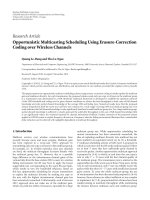
Examples of Gaussian TF functions with different scales
and modulation parameters are shown in Figure 1.The
order of computational complexity for one iteration of the
ATFT algorithm is given by O(N log N)whereN is the
length of the signal samples. The time complexity of the
ATFT algorithm increases with the increase in the number
of iterations required to model a signal, which in turn
depends on the nature of the signal. Compared to this
the computational complexity of Modified Discrete Cosine

Transform (MDCT) used in few of the state-of-the-art audio
coders is only O(N log N) (same as FFT).
Once the signal is modeled accurately or decomposed
into TF functions with definite time and frequency localiza-
tion, the TF parameters governing the TF functions could
be analyzed for extracting application-specific information.
In our case we process the TF decomposition parameters of
the audio signals to perform both audio compression and
classification as will be explained in the later sections.
2.2. TF Distribution Approach. TF distribution (TFD) indi-
cates a two-dimensional energy representations of a signal in
terms of time-and frequency-domains. The work in the area
of TFD methods is extensive [2, 5–7]. Some well-known TFD
techniques are as follows.
2.2.1. Linear TFDs. The simplest linear TFD is the squared
modulus of STFT of a signal, which assumes that the
signal is stationary in short durations and multiplies the
signal by a window, and takes the Fourier transform on the
windowed segments. This joint TF representation represents
the localization of frequency in time; however, it suffers from
TF resolution tradeoff.
2.2.2. Quadratic TFDs. In quadratic TFDs, the analysis
window is adapted to the analyzed signal. To achieve this, the
quadratic TFD transforms the time varying autocorrelation
of the signal to obtain a representation of the signal energy
distributed over time and frequency
X
WV
(
τ, ω

)
=

x

t +
1
2
τ

x
∗

t −
1
2
τ

exp

−
jωt

dt,(4)
where X
WV
is Wigner-Ville distribution (WVD) of the
signal. WVD offers higher resolution than STFT; however,
when more than one component exists in the signal, the
WVD contains interference cross terms. Interference cross

terms do not belong to the signal and are generated by
the quadratic nature of the WVD. They generate highly
oscillatory interference in the TFD, and their presence will
lead to incorrect interpretation of the signal properties.
This drawback of the WVD is the motivation for introduc-
ing other TFDs such as Pseudo Wigner-Ville Distribution
(PWVD), SPWVD, Choi-Williams Distribution (CWD), and
Cohen kernel distribution to define a kernel in ambiguity
domain that can eliminate cross terms. These distributions
belong to a general class called the Cohens class of bilinear
TF representation [3].TheseTFDsarenotalwayspositive.
In order to produce meaningful features, the value of the
TFD should be positive at each point; otherwise the extracted
features may not be interpretable, for example, the WVD
always results in positive instantaneous frequency, but it
also gives that the expectation value of the square of the
frequency, for a fixed time, can become negative which does
not make any sense [8]. Additionally, it is very difficult to
explain negative probabilities.
2.2.3. Positive TFDs. They produce non-negative TFD of a
signal, and do not contain any cross terms. Cohen and Posch
[8] demonstrate the existence of an infinite set of positive
TFDs, and developed formulations to compute the positive
TFDs based on signal-dependent kernels. However, in order
to calculate these kernels, the method requires the signal
equation which is not known in most of the cases. Therefore,
although positive TFDs exist, their derivation process is very
complicated to implement.
4 EURASIP Journal on Advances in Signal Processing
Time position

p
n
Centre frequency
f
n
Higher
centre frequency
Scale or octave
s
n
TF functions with
smaller scale
Figure 1: Gaussian TF function with different scale, and modulation parameters.
2.2.4. Matching Pursuit TFD. (MP-TFD) is constructed from
matching pursuit as proposed by Mallat and Zhang [2]in
1993. As shown in (3), matching pursuit decomposes a
signal into Gabor atoms with a wide variety of frequency
modulated, phase and time shift, and duration. After M
iteration, the selected components may be concluded to
represent coherent structures, and the residue represents
incoherent structures in the signal. The residue may be
assumed to be due to random noise, since it does not show
any TF localization. Therefore, in MP-TFD, the decompo-
sition residue in (3) is ignored, and the WVD of each M
component is added as the following:
X
(
τ, ω
)
=

M−1

n=0




R
n
x
, g
γ
n




2
Wg
γ
n
(
τ, ω
)
,
(5)
where Wg
γ
n
(τ, ω) is the WVD of the Gabor atom g

γ
n
(t),
and X(τ, ω) is the constructed MP-TFD. As previously
mentioned, the WVD is a powerful TF representation;
however when more than one component is present in the
signal, the TF resolution will be confounded by cross terms.
In MP-TFD, we apply the WVD to single components and
add them up, therefore, the summation will be a cross-term
free distribution.
Despite the potential advantages of TFD to quantify
nonstationary information of real world signals, they have
been mainly used for visualization purposes. We review the
TFD quantification in the next section, and then we explain
our proposed TFD quantification method.
2.3. TFD-Based Quantification. There have been some
attempts in literature to TF quantification by removing the
redundancy and keeping only the representative parts of the
TFD. In [9], the authors consider the TF representation of
music signals as texture images, and then they look for the
repeating patterns of a given instrument as the representative
feature of that instrument. This approach is useful for music
signals; however, it is not very efficient for environmental
sound classification, where we can not assume the presence
of such a structured TF patterns.
Another TF quantification approach is obtaining the
instantaneous features from the TFD. One of the first works
in this area is the work of Tacer and Loughlin [10], in
which Tacer and Loughlin derive two-dimensional moments
of the TF plane as features. This approach simply obtains

one instantaneous feature for every temporal sample as
related to spectral behavior of the signal at each point.
However, the quantity of the features is still very large.
In [11, 12], instead of directly applying the instantaneous
features in the classification process, some statistical prop-
erties of these features (e.g., mean and variance) are used.
Although this solution reduces the dimension of instanta-
neous features, its shortcoming is that the statistical analysis
diminishes the temporal localization of the instantaneous
features.
In a recent approach, the TFD is considered as a matrix,
and then a matrix decomposition (MD) technique is applied
to the TF matrix (TFM) to derive the significant TF com-
ponents. This idea has been used for separating instruments
in music [13, 14], and has been recently used for music
classification [15]. In this approach, the base components
are used as feature vectors. The major disadvantage of this
method is that the decomposed base vectors have a high
dimension, and as a result they are not very appealing
features for classification purposes.
EURASIP Journal on Advances in Signal Processing 5
Figure 2 depicts our proposed TF quantification
approach. As shown in this figure, signal (x(t)) is
transformed into TF matrix V,whereV is the TFD of
signal x(t)(V
= X(τ, ω)). Next, a MD is applied to the TFM
to decompose the TF matrix into its base and coefficient
matrices (W and H, resp.) in a way that V
= W × H.We
then extract some features from each vector of the base

matrix, and use them as joint TF features of the signal (x(t)).
This approach significantly reduces the dimensionality
of the TFD compared to the previous TF quantification
approaches. We call the proposed methodology as TFM
decomposition feature extraction technique. In our previous
paper [16], we applied TF decomposition feature extraction
methodology to speech signals in order to automatically
identify and measure the speech pathology problem. We
extracted meaningful and unique features from both base
and coefficient matrices. In this work, we showed that the
proposed method extracts meaningful and unique joint
TF features from speech, and automatically identifies and
measures the abnormality of the signal. We employed TFM
decomposition technique to quantify TFD, and proposed
novel features for environmental audio signal classification
[17]. Our aim in the present work is to extract novel TF
features, based on TFM decomposition technique in an
attempt to increase the accuracy of the environmental audio
classification.
2.4. TFM Decomposition. The TFM of a signal x(t)isdenoted
with V
K×N
,whereN is signal length and K is frequency
resolution in the TF analysis. An MD technique with r
decomposition is applied to a matrix in such a way that each
element in the TFM can be written as follows:
V
K×N
= W
K×r

H
r×N
=
r

i=1
w
i
h
i
,
(6)
where the decomposed TF matrices, W and H,aredefinedas:
W
K×r
=
[
w
1
w
2
···w
r
]
,
H
r×N
=
⎡
⎢

⎢
⎢
⎢
⎢
⎢
⎢
⎣
h
1
h
2
.
.
.
h
r
⎤
⎥
⎥
⎥
⎥
⎥
⎥
⎥
⎦
.
(7)
In (6), MD reduces the TF matrix (V) to the base and
coefficient vectors (
{w

i
}
i=1, ,r
and {h
i
}
i=1, ,r
,resp.)inaway
that the former represents the spectral components in the TF
signal structure, and the latter indicates the location of the
corresponding spectral component in time.
There are several well-known MD techniques in liter-
ature, for example, Principal Component Analysis (PCA),
Independent Component Analysis (ICA), and Non-negative
Matrix Factorization (NMF). Each MD technique considers
different sets of criteria to choose the decomposed matrices
with the desired properties, for example, PCA finds a set
of orthogonal bases that minimize the mean squared error
of the reconstructed data; ICA is a statistical technique that
decomposes a complex dataset into components that are as
independent as possible; and NMF technique is applied to a
non-negative matrix, and decomposes the matrix to its non-
negative components.
A MD technique is suitable for TF quantification that the
decomposed matrices produce representative and meaning-
ful features. In this work, we choose NMF as the MD method
because of the following two reasons.
(1) In a previous study [18], we showed that the
NMF components promise a higher representation and
localization property compared to the other MD techniques.

Therefore, the features extracted from the NMF component
represent the TFM with a high-time and-frequency localiza-
tion.
(2) NMF decomposes a matrix into non-negative com-
ponents. Negative spectral and temporal distributions are
not physically interpretable and therefore do not result in
meaningful features. Since PCA and ICA techniques do not
guarantee the non-negativity of the decomposed factors,
instead of directly using W and H matrices to extract
features, their squared values,

W and

H are used [19]. In
other words, rather than extracting the features from V
≈
WH, the features are extracted from TFM of

V as defined
below

V ≈
r

i=1


w
i


f



|
h
i
(
t
)
|. (8)
It can be shown that

V
/
=V, and the negative elements of W
and H cause artifacts in the extracted TF features. NMF is
the only MD techniques that guarantees the non-negativity
of the decomposed factors and it therefore is a better MD
technique to extract meaningful features compared to ICA
and PCA. Therefore, NMF is chosen as the MD technique in
TFM decomposition.
NMF algorithm starts with an initial estimate for W and
H, and performs an iterative optimization to minimize a
given cost function. In [20], Lee and Seung introduce two
updating algorithms using the least square error and the
Kullback-Leibler (KL) divergence as the cost functions.
Least square error:
W
←− W ·

VH
T
WHH
T
, H ←− H ·
W
T
V
W
T
WH
.
KL divergence:
W
←− W ·
(
V/WH
)
H
T
1 ·H
, H
←− H ·
W
T
(
V/WH
)
W ·1
.

(9)
In these equations,
· and /are term by term multi-
plication and division of two matrices. Various alternative
minimization strategies for NMF decomposition have been
proposed in [21, 22]. In this work, we use a projected gradi-
ent bound-constrained optimization method by Lin in [23].
The gradient-based NMF is computationally competitive
and offers better convergence properties than the standard
approach.
6 EURASIP Journal on Advances in Signal Processing
Tr ai n
MP-TFD
Audio signal
x(t)
V
M×N
W
M×r
H
r×N
NMF
Feature
extraction
F
r×20
F
r×20
LDA
classifier

{C}
Te s t
Audio signal
x(t)
MP-TFD
V
M×N
NMF
Feature
extraction
LDA
classifier
W
M×r
H
r×N
1. Aircraft
2. Helicopter
3. Drum
4. Flute
5. Piano
6. Male
7. Female
8. Animal
9. Bird
10. Insect
Figure 2: This block diagram represents the TFM quantification technique. In this approach, first the TFD (V
K×N
)ofasignal(x(t)) is
estimated. Then a MD technique decomposes the estimated TF matrix into r bases components (W

K×r
and H
r×N
). Finally, a discriminant
and representative feature vector F is extracted from each decomposed component.
Wideband
audio
TF
modeling
TF
parameter
processing
Perceptual filtering
Threshold
in
quiet
(TIQ)
Masking
Quantizer
Media
or
channel
Figure 3: Block diagram of ATFT audio coder.
We apply the TFM decomposition of the audio signals to
perform environmental audio classification as is explained in
Section 4.2.
3. Audio Coding
In order to address the high demand for audio com-
pression, over the years many compression methodologies
were introduced to reduce the bit rates without sacrificing

much of the audio quality. Since it is out of scope of
this paper to cover all of the existing audio compression
methodologies, the authors recommend the work of Painter
and Spanias in [24] for a comprehensive review of most
of the existing audio compression techniques. Audio signals
are highly nonstationary in nature and the best way to
analyze them is to use a joint TF approach. The presented
coding methodology is based on ATFT and falls under the
transform-like coder category. The usual methodology of
a transform-based coding technique involves the following
steps: (i) transforming the audio signal into frequency
or TF-domain coefficients, (ii) processing the coefficients
using psychoacoustic models and computing the audio
masking thresholds, (iii) controlling the quantizer resolution
using the masking thresholds, (iv) applying intelligent bit
allocation schemes, and (v) enhancing the compression ratio
with further lossless compression schemes. The ATFT-based
coder nearly follows the above general transform coder
methodology; however, unlike the existing techniques, the
major part of the compression was achieved by exploiting
the joint TF properties of the audio signals. The block
diagram of the ATFT coder is shown in Figure 3.TheATFT
approach provides higher TF resolution than the existing TF
techniques such as wavelets and wavelet packets [2]. This
high-resolution sparse decomposition enables us to achieve a
compact representation of the audio signal in the transform
domain itself. Also, due to the adaptive nature of the ATFT,
there was no need for signal segmentation.
Psychoacoustics were applied in a novel way on the TF
decomposition parameters to achieve further compression.

In most of the existing audio coding techniques the funda-
mental decomposition components or building blocks are in
the frequency domain with corresponding energy associated
with them. This makes it much easier for them to adapt
the conventional, well-modeled psychoacoustics techniques
into their encoding schemes. On the other hand, in ATFT,
the signal was modeled using TF functions which have a
definite time and frequency resolution (i.e., each individual
TF function is time limited and band limited), hence the
existing psychoacoustics models need to be adapted to apply
on the TF functions [25].
3.1. ATFT of Audio Signals. Any signal could be expressed
as a combination of coherent and noncoherent signal
structures. Here the term coherent signal structures means
those signal structures that have a definite TF localization
(or) exhibit high correlation with the TF dictionary elements.
In general, the ATFT algorithm models the coherent signal
structures well within the first few 100 iterations, which
in most cases contribute to >90% of the signal energy.
On the other hand, the noncoherent noise-like structures
EURASIP Journal on Advances in Signal Processing 7
cannot be easily modeled since they do not have a definite
TF localization or correlation with dictionary elements.
Hence these noncoherent structures are broken down by
the ATFT into smaller components to search for coherent
structures. This process is repeated until the whole residue
information is diluted across the whole TF dictionary [2].
From a compression point of view, it would be desirable
to keep the number of iterations (M ≪ N), as low as
possible and at the same time sufficient enough to model

the audio signal without introducing perceptual distortions.
Considering this requirement, an adaptive limit has to be set
for controlling the number of iterations. The energy capture
rate (signal energy capture rate per iteration) could be used
to achieve this. By monitoring the cumulative energy capture
over iterations we could set a limit to stop the decomposition
when a particular amount of signal energy was captured.
The minimum number of iterations required to model
an audio signal without introducing perceptual distortions
depends on the signal composition and the length of the
signal. In theory, due to the adaptive nature of the ATFT
decomposition, it is not necessary to segment the signals.
However, due to the computational resource limitations
(Pentium III, 933 MHZ with 1 GB RAM), we decomposed
the audio signals in 5 s durations. The larger the duration
decomposed, the more efficient is the ATFT modeling. This
is because if the signal is not sufficiently long, we cannot
efficiently utilise longer TF functions (highest possible scale)
to approximate the signal. As the longer TF functions cover
larger signal segments and also capture more signal energy
in the initial iterations, they help to reduce the total number
of TF functions required to model an audio signal. Each
TF function has a definite time and frequency localization,
which means all the information about the occurrences of
each of the TF functions in time and frequency of the
signal is available. This flexibility helps us later in our
processing to group the TF functions corresponding to any
short time segments of the audio signal for computing the
psychoacoustic thresholds. In other words, the complete
length of the audio signal can be first decomposed into TF

functions and later the TF functions corresponding to any
short time segment of the signal can be grouped together.
In comparison, most of the DCT- and MDCT-based existing
techniques have to segment the signals into time frames and
process them sequentially. This is needed to account for the
non-stationarity associated with the audio signals and also to
maintain a low signal delay in encoding and decoding.
In the presented technique for a signal duration of 5 s, the
decomposition limit was set to be the number of iterations
(M
x
) needed to capture 99.5% of the signal energy or to a
maximum of 10,000 iterations and is given by
M
x
=
⎧
⎪
⎪
⎪
⎨
⎪
⎪
⎪
⎩
M,ifM<10000, .995=

M−1
n
=0





R
n
x, g
γ
n




2

∞
−∞
|x
(
t
)
|
2
dt
,
10000, otherwise.
(10)
For a signal with less noncoherent structures, 99.5% of
signal energy could be modeled with a lower number of TF
functions than a signal with more noncoherent structures. In

most cases a 99.5% of energy capture nearly characterises the
audio signal completely. The upper limit of the iterations is
fixed to 10,000 iterations to reduce the computational load.
Figure 4 demonstrates the number of TF functions needed
for a sample audio signal. In the figure, the lower panel shows
the energy capture curve for the sample audio signal in the
top panel with number of TF functions in the X-axis and the
normalised energy in the Y-axis. On average, it was observed
that 6000 TF functions are needed to represent a signal of 5 s
duration sampled at 44.1 kHz.
3.2. Implementation of Psychoacoustics. In the conventional
coding methods, the signal is segmented into short time
segments and transformed into frequency domain coeffi-
cients. These individual frequency components are used
to compute the psychoacoustic masking thresholds and
accordingly their quantization resolutions are controlled.
In contrast, in our approach we computed the psychoa-
coustic masking properties of individual TF functions and
used them to decide whether a TF function with certain
energy was perceptually relevant or not based on its time
occurrence with other TF functions. TF functions are the
basic components of the presented technique and each TF
function has a certain time and frequency support in the
TF plane. So their psychoacoustical properties have to be
studied by taking them as a whole to arrive at a suitable
psychoacoustical model. More details on the implementation
of psychoacoustics is covered in [25, 26].
3.3. Quantization. Most of the existing transform-based
coders rely on controlling the quantizer resolution based on
psychoacoustic thresholds to achieve compression. Unlike

this, the presented technique achieves a major part of
the compression in the transformation itself followed by
perceptual filtering. That is, when the number of iterations
M needed to model a signal is very low compared to the
length of the signal, we just need M
× L bits. Where L is the
number of bits needed to quantize the 5 TF parameters that
represent a TF function. Hence, we limited our research work
to scalar quantizers as the focus of the research mainly lies on
the TF transformation block and the psychoacoustics block
rather than the usual sub-blocks of the data compression
application.
As explained earlier each of the five parameters Energy
(a
n
), Center frequency ( f
n
), Time position (p
n
), Octave
(s
n
), and Phase (φ
n
) are needed to represent a TF function
and thereby the signal itself. These five parameters were
to be quantized in such a way that the quantization error
introduced was imperceptible while, at the same time,
obtaining good compression. Each of the five parameters
has different characteristics and dynamic range. After careful

analysis of them the following bit allocations were made. In
arriving at the final bit allocations informal Mean Opinions
Score (MOS) tests were conducted to compare the quality of
the audio samples before and after quantization stage.
In total, 54 bits are needed to represent each TF func-
tion without introducing significant perceptual quantization
8 EURASIP Journal on Advances in Signal Processing
−0.2
−0.1
0
0.1
0.2
Amplitude (a.u.)
0.20.40.60.811.21.41.61.822.2
×10
5
Time samples
Sample signal
(a)
0
0.2
0.4
0.6
0.8
1
×10
−3
Energy (a.u.)
0 1000 2000 3000 4000 5000 6000 7000 8000 9000 10000
Number of TF functions

Energy curve
99.5% of the signal energy
(b)
Figure 4: Energy cutoff of the sample signal in panel 1. a.u.: arbitrary units.
noise in the reconstructed signal. The final form of data for
M TF functions will contain the following.
(i) Energy parameter (Log companded)
= M ∗12 bits.
(ii) Time position parameter
= M ∗15 bits.
(iii) Center frequency parameter
= M ∗13 bits.
(iv) Phase parameter
= M ∗10 bits.
(v) Octave parameter
= M ∗4 bits.
Thesumofalltheabove(
= 54 ∗ M bits) will be the
total number of bits transmitted or stored representing an
audio segment of duration 5 s. The energy parameter after
log companding was observed to be a very smooth curve.
Fitting a curve to the energy parameter further reduces
the bit rate [25, 26]. With just a simple scalar quantizer
and curve fitting of the energy parameter, the presented
coder achieves high-compression ratios. Although a scalar
quantizer was used to reduce the computational complexity
of the presented coder, sophisticated vector quantization
techniques can be easily incorporated to further increase the
coding efficiency. The 5 parameters of the TF function can
be treated as one vector and accordingly quantized using

predefined codebooks. Once the vector is quantized, only the
index of the codebook needs to be transmitted for each set
of TF parameters resulting in a large reduction of the total
number of bits. However designing the codebooks would be
challenging as the dynamic ranges of the 5 TF parameters
are drastically different. Apart from reducing the number
of total bits, the quantization stage can also be utilized to
control the bit rates suitable for CBR (Constant Bit Rate)
applications.
3.4. Compression Ratios. Compression ratios achieved by the
presented coder were computed for eight sample wideband
audio signals (of 5 s duration) as described below. These
eight sample signals (namely, ACDC, DEFLE, ENYA, HARP,
HARPSICHORD, PIANO, TUBULARBELL, and VISIT)
were representatives of wide range of music types.
(i) As explained earlier, the total number of bits needed
to represent each TF function is 54.
(ii) The energy parameter is curve fitted and only the first
150 points in addition to the curve fitted point need
to be coded.
(iii) So the total number of bits needed for M iterations
for a 5 s duration of the signal is TB
1
= (M ∗ 42) +
((150 + C)
∗ 12), where C is the number of curve
fitted points, and M is the number of perceptually
important functions.
(iv) The total number of bits needed for a CD quality 16
bit PCM technique for a 5 s duration of the signal

sampled at 44100 Hz is TB
2
= 44100 ∗ 5 ∗ 16 =
3, 528, 000.
(v) The compression ratio can be expressed as the ratio of
number of bits needed by the presented coder to the
number of bits needed by the CD quality 16 bit PCM
technique for the same length of the signal, that is,
Compression ratio
=
TB
2
TB
1
. (11)
(vi) The overall compression ratio for a signal was then
calculated by averaging all the 5 s duration segments
of the signal for both the channels.
EURASIP Journal on Advances in Signal Processing 9
The presented coder is based on an adaptive signal trans-
formation technique, that is, the content of the signal and the
dictionary of basis functions used to model the signal play an
important role in determining how compact a signal can be
represented (compressed). Hence, VBR (Variable Bit Rate) is
the best way to present the performance benefit of using an
adaptive decomposition approach. The inherent variability
introduced in the number of TF functions required to model
a signal and thereby the compression is one of the highlights
of using ATFT. Although VBR would be more appropriate to
present the performance benefit of the presented coder, CBR

mode has its own advantages when using with applications
that demand network transmissions over constant bitrate
channels with limited delays. The presented coder can also
be used in CBR mode by fixing the number of TF functions
used for representing signal segments, however due to the
signal adaptive nature of the presented coder this would
compromise the quality at instances where signal segments
demand a higher number of TF functions for perceptually
lossless reproduction. Hence we choose to present the results
of the presented coder using only the VBR mode.
We compared the presented coder with two existing
popular and state-of-the-art audio coders, namely, MP3
(MPEG 1 layer 3) and MPEG-4 AAC/HE-AAC. Advanced
audio coding (AAC) is the current industrial standard which
was initially developed for multichannel surround signals
(MPEG-2 AAC [27]). As there are ample studies in the
literature [27–32] available for both MP3 and MPEG-2/4
AAC more details about these techniques are not provided
in this paper. The average bit rates were used to calculate
the compression ratio achieved by MP3 and MPEG-4 AAC
as described below.
(i) Bitrate for a CD quality 16 bit PCM technique for 1 s
stereo signal is given by TB
3
= 2 ∗44100 ∗16.
(ii) The average bit rate/s achieved by (MP3 or MPEG-4
AAC) in VBR mode
= TB
4
.

(iii) Compression ratio achieved by (MP3 or MPEG-4
AAC)
= TB
3
/TB
4
.
The 2nd, 4th and 6th columns of Ta bl e 1 show the
compression ratio (CR) achieved by the MP3, MPEG-4 AAC
and the presented ATFT coders for the set of 8 sample audio
files. It is evident from the table that the presented coder has
better compression ratios than MP3. When comparing with
MPEG-4 AAC, 5 out of 8 signals are either comparable or
have better compression ratios than the MPEG-4 AAC. It is
noteworthy to mention that for slow music (classical type)
the ATFT coder provides 3 to 4 times better comparison than
MPEG-4 AAC or MP3.
The compression ratio alone cannot be used to evaluate
an audio coder. The compressed audio signals has to undergo
a subjective evaluation to compare the quality achieved
with respect to the original signal. The combination of the
subjective rating and the compression ratio will provide a
true evaluation of the coder performance.
Before performing the subjective evaluation, the signal
has to be reconstructed. The reconstruction process is a
Table 1: Compression ratio (CR) and subjective difference grades
(SDGs). MP3: Moving Picture Experts Group I Layer 3, MPEG-4
AAC: Moving Picture Experts Group 4 Advanced Audio Coding,
VBR Main LTP profile, and ATFT: Adaptive Time-Frequency
Tr an sf or m.

Samples
MP3 AAC ATFT
CR SDG CR SDG CR SDG
ACDC 7.5 0.067 9.3 −0.067 8.4 −0.93
DEFLE 7.7
−0.2 9.5 −0.067 8.3 −1.73
ENYA 9 0 9.6
−0.133 20.6 −0.8
HARP 11
−0.067 9.4 −0.067 36.3 −1
HARPSICHORD 8.5
−0.067 10.2 0.33 9.3 −0.73
PIANO 13.6 0.067 9.6
−0.2 40 −0.8
TUBULARBELL 8.3 0 10.1 0.067 10.5
−0.53
VISIT 8.4
−0.067 11.5 0 11.6 −2.27
AV E R AG E 9 . 3 −0.03 9.9 −0.02 18.3 −1.1
straightforward process of linearly adding all the TF func-
tions with their corresponding five TF parameters. In order
to do that, first the TF parameters modified for reducing
the bit rates have to be expanded back to their original
forms. The log compressed energy curve was log expanded
after recovering back all the curve points using interpolation
on the equally placed 50 length points. The energy curve
was multiplied with the normalization factor to bring the
energy parameter as it was during the decomposition of
the signal. The restored parameters (Energy, Time-position,
Center frequency, Phase and Octave) were fed to the ATFT

algorithm to reconstruct the signal. The reconstructed signal
was then smoothed using a 3rd-order Savitzky-Golay [33]
filter and saved in a playable format.
Figure 5 demonstrates a sample signal (/“HARP”/) and
its reconstructed version and the corresponding spectro-
grams. It can be clearly observed from the reconstructed
signal spectrogram compared with the original signal spec-
trogram, how accurately the ATFT technique has filtered
out the irrelevant components from the signal (evident
from Tabl e 1—(/“HARP”/)—high-compression ratio versus
acceptable quality). The accuracy in adaptive filtering of the
irrelevant components is made possible by the TF resolution
provided by the ATFT algorithm.
3.5. Subjective Evaluation of ATFT Coder. Subjective evalu-
ation of audio quality is needed to assess the audio coder
performance. Even though there are objective measures such
as SNR, total harmonic distortion (THD), and Noise-to-
mask ratio [34] they would not give a true evaluation of the
audio codec particularly if they use lossy schemes as in the
proposed technique. This is due to the fact say, for example,
in a perceptual coder, SNR is lost however audio quality is
claimed to be perceptually lossless. In this case SNR measure
may not give the correct performance evaluation of the coder.
We used the subjective evaluation method recommended
by ITU-R standards (BS. 1116). It is called a “double blind
triple stimulus with hidden reference” [24, 34]. A Subjective
10 EURASIP Journal on Advances in Signal Processing
−0.2
−0.1
0

0.1
0.2
Amplitude (a.u.)
1234
×10
5
Time samples
Original
(a)
0
0.5
1
1.5
2
×10
4
Frequency (Hz)
02468
Time (s)
Original
(b)
−0.2
−0.1
0
0.1
0.2
Amplitude (a.u.)
1234
×10
5

Time samples
Reconstructed
(c)
0
0.5
1
1.5
2
×10
4
Frequency (Hz)
02468
Time (s)
Reconstructed
(d)
Figure 5: Example of a sample original (/“HARP”/) and the reconstructed signal with their respective spectrograms. X-axes for the original
and reconstructed signal are in time samples, and X-axes for the spectrogram of the original and the reconstructed signal are in equivalent
time in seconds. Note that the sampling frequency
= 44.1 kHz. au: arbitrary units.
Difference Grade (SDG) [24] was computed by subtracting
the absolute score assigned to the hidden reference audio
signal from the absolute score assigned to the compressed
audio signal. It is given by
SDG
= Grade
{compressed}
−Grade
{reference}
. (12)
Accordingly the scale of SDG will range from (

−4to
0) with the following interpretation: (
−4): Unsatisfactory
(or) Very Annoying, (
−3): Poor (or) Annoying, (−2): Fair
(or) Slightly annoying, (
−1): Good (or) Perceptible but
not annoying, and (0): Excellent (or) Imperceptible. Fifteen
listeners (randomly selected) participated in the MOS studies
and evaluated all the 3 audio coders (MP3, AAC and ATFT
in VBR mode). The average SDG was computed for each
of the audio sample. The 3rd, 5th and 7th columns of the
Ta bl e 1 show the SDGs obtained for MP3, AAC and ATFT
coders, respectively. MP3 and AAC SDGs fall very close to the
Imperceptible (0) region, whereas the proposed ATFT SDGs
are spread out between
−0.53 to −2.27.
EURASIP Journal on Advances in Signal Processing 11
3.6. Results and Discussion. The compression ratios (CRs)
and the SDG for all three coders (MP3, AAC and ATFT)
are shown in Ta b le 1 . All the coders were tested in the VBR
mode. For the presented technique, VBR was the best way
to present the performance benefit of using an adaptive
decomposition approach. In ATFT, the type of the signal and
the characteristics of the TF functions (type of dictionary)
control the number of transformation parameters required
to approximate the signal and thereby the compression ratio.
The inherent variability introduced in the number of TF
functions required to model a signal is one of the highlights
of using ATFT. Hence we choose to present comparison of

the coders in the VBR mode.
The results show that the MP3 and AAC coders per-
form well with excellent SDG scores (Imperceptible) at a
compression ratio around 10. The presented coder does
not perform well with all of the eight samples. Out of
the 8 samples, 6 samples have an SDG between
−0.53 to
−1 (Imperceptible—perceptible but not annoying) and 2
samples have SDG below
−1. Out of the 6 samples with
SDGs between (
−0.53 and −1), 3 samples (ENYA, HARP and
PIANO) have compression ratios 2 to 4 times higher than
MP3 and AAC and 3 samples (ACDC, HARPSICHORD and
TUBULARBELL) have comparable compression ratios with
moderate SDGs.
Figure 6 shows the comparison of all three coders
by plotting the samples with their SDGs in X-axis and
compression ratios in the Y-axis. If we can virtually divide
this plot in segments of SDGs (horizontally) and the
compression ratios (vertically), then the ideal desirable coder
performance should be in the right top corner of the plot
(high-compression ratios and excellent SDG scores). This is
followed next by the right bottom corner (low-compression
ratios and excellent SDG scores) and so on as we move from
right to left in the plot. Here the terms “Low”- and “High”-
compression ratios are used in a relative sense based on the
compression ratios achieved by all the 3 coders in this study.
From the plot it can be seen that MP3 and AAC coders
occupy the right bottom corner, whereas the samples from

ATFT coder are spread over. As mentioned earlier 3 out the 8
samples of the ATFT coder occupy the right top corner only
with moderate SDGs that are much less than the MP3 and
the AAC. 3 out of the remaining 5 samples of the ATFT coder
occupy the right bottom corner, again with only moderate
SDGs that are less than MP3 and AAC. The remaining 2
samples perform the worst occupying the left bottom corner.
We analyzed the poorly performing ATFT coded signals
DEFLE and VISIT. DEFLE is a rapidly varying rock-like
signal with minimal voice components and VISIT is a signal
with dominant voice components. We observed that the
symmetrical and smooth Gaussian dictionary used in this
study does not model the transients well, which are the
main features of all rapidly varying signals like DEFLE.
This inefficient modeling of transients by the symmetrical
Gaussian TF functions resulted in the poor SDG for the
DEFLE. A more appropriate dictionary would be a damped
sinusoids dictionary [35] which can better model the
transient-like decaying structures in audio signals. However
a single dictionary alone may not be sufficient to model
5
10
15
20
25
30
35
40
45
Compression ratio (CR)

−4 −3 −2 −10 1
Very annoying Imperceptible
Subjective difference grade (SDG)
Subjective difference grade (SDG) versus
compression ratios (CR)
MP3
AAC
ATFT
Figure 6: Subjective Difference Grade (SDG) versus Compression
ratios (CRs).
all types of signal structures. The second signal VISIT has
significant amount(s) of voice components. Even though
the main voice components are modeled well by the ATFT,
the noise-like hissing and shrilling sounds (noncoherent
structures) could not be modeled within the decomposition
limit of 10,000 iterations. These hissing and shrilling sounds
actually add to the pleasantness of the music. Any distortion
in them is easily perceived which could have reduced the
SDG of the signal to the lowest of the group
−2.27. The
poor performances with the two audio sample cases could
be addressed by using a hybrid dictionary of TF functions
and residue coding the noncoherent structures separately.
However this would increase the computational complexity
of the coder and reduce the compression ratios.
We have covered most details involved in a stage by
stage implementation and evaluation of a transform-based
audio coder. The approach demonstrated the application
of ATFT for audio coding and the development of a
novel psychoacoustics model adapted to TF functions. The

compression strategy was changed from the conventional
way of controlling quantizer resolution to achieving majority
of the compression in the transformation itself. Listening
tests were conducted and the performance comparison of the
presented coder with MP3 and AAC coders were presented.
From the preliminary results, although the proposed coder
achieves high-compression ratios, its SDG scores are well
below the MP3 and AAC family of coders. The proposed
coder however performs moderately well for slowly varying
classical type signals with acceptable SDGs. The proposed
coder is not as refined as the state-of-the-art commercial
coders, which to some extent explains its poor performance.
12 EURASIP Journal on Advances in Signal Processing
From the results presented for the ATFT coder, the
signal adaptive performance of the coder for a specific
TF dictionary is evident, that is, with a Gaussian TF
dictionary the coder performed moderately well for slow-
varying classical signals than fast varying rock-like signals.
In other words the ATFT algorithm demonstrated notable
differences in the decomposition patterns of classical and
rock-like signals. This is a valid clue and a motivating
factor that these differences in the decomposition patterns if
quantified using TF decomposition parameters could be used
as discriminating features for classifying audio signals. We
apply this hypothesis in extracting TF features for classifying
audio signals for a content-based audio retrieval application
as will be explained in Section 4.
3.7. Summary of Steps Involved in Implementing
ATFT Audio Coder
Step 1 (ATFT algorithm and TF dictionaries). Existing

implementation of Matching Pursuits can be adapted for the
purposes; (1) LastWave ( />∼bacry/LastWave/), (2) Matching Pursuit Package (MPP)
( and (3)
Matching Pursuit ToolKit (MPTK) [36].
Step 2 (Control decomposition). The number of TF func-
tions required to model a fixed segment of audio signal can
be arrived using similar criteria described in Section 3.1.
Step 3 (Perceptual Filtering). The TF functions obtained
from Step 2 can be further filtered using the psychoacoustics
thresholds discussed in Section 3.2.
Step 4 (Quantization). The simple quantization scheme
presented in Section 3.3 canbeusedforbitallocationor
advanced vector quantization methods can also be explored.
Step 5 (Lossless schemes). Further lossless schemes can be
applied to the quantized TF parameters to further increase
the compression ratio.
4. Audio Classification
Audio feature extraction plays an important role in analyzing
and characterizing audio content. Auditory scene analysis,
content-based retrieval, indexing, and fingerprinting of
audio are few of the applications that require efficient feature
extraction. The general methodology of audio classification
involves extracting discriminatory features from the audio
data and feeding them to a pattern classifier. Different
approaches and various kinds of audio features were pro-
posed with varying success rates. Audio feature extraction
serves as the basis for a wide range of applications in the areas
of speech processing [37], multimedia data management and
distribution [38–41], security [42], biometrics and bioacous-
tics [43]. The features can be extracted either directly from

the time-domain signal or from a transformation domain
depending upon the choice of the signal analysis approach.
Some of the audio features that have been successfully
Audio
signal
Adaptive
signal
decomposition
Feature
extraction
Linear
discriminant
analysis
Rock
Classical
Country
Folk
Jazz
Pop
Figure 7: Block diagram of the proposed music classification
scheme.
used for audio classification include mel frequency cepstral
coefficients (MFCCs) [40, 41], spectral similarity [44],
timbral texture [41], band periodicity [38], LPCC (Linear
Prediction Coefficient-derived cepstral coefficients) [45],
zero crossing rate [38, 45], MPEG-7 descriptors [46], entropy
[12], and octaves [39]. Few techniques generate a pattern
from the features and use it for classification by the degree
of correlation. Few other techniques use the numerical
values of the features coupled to statistical classification

methods.
4.1. Music Classification. In this section, we present a
content-based audio retrieval application employing audio
classification and explain the generic steps involved in
performing successful audio classification. The simplest of
all retrieval techniques is the text-based searching where the
information about the multimedia data is stored with the
data file. However the success of these type of text-based
searches depend on how well they are text indexed by the
author and they do not provide any information on the real
content of the data. To make the retrieval system automated,
efficient, and intelligent, content-based retrieval techniques
were introduced. The presented work focuses on one such
way for automatic classification of audio signals for retrieval
purposes. The block diagram of the proposed technique is
shown in Figure 7.
In content-based retrieval systems, audio data is ana-
lyzed, and discriminatory features are extracted. The selec-
tion of features depends on the domain of analysis and
the perceptual characteristics of the audio signals under
consideration. These features are used to generate subspaces
dividing the audio signal types to fit in one of the subspaces.
The division of subspaces and the level of classification vary
from technique to technique. When a query is placed the
similarity of the query is checked with all subspaces and
the audio signals from the highly correlated subspace is
returned as the result. The classification accuracy, and the
discriminatory power of the features extracted determine the
success of such retrieval systems.
Most of the existing techniques do not take into con-

sideration the true nonstationary behavior of the audio
signals while deriving their features. The presented approach
uses the same ATFT transform that was discussed in the
previous audio coding section. ATFT approach is one of the
best ways to handle nonstationary behavior of the audio
signals and also due to its adaptive nature, does not require
any signal segmentation techniques as used by most of the
existing techniques. Unlike many existing techniques where
EURASIP Journal on Advances in Signal Processing 13
−0.2
−0.1
0
0.1
0.2
Amplitude (a.u.)
0.20.40.60.811.21.41.61.822.2
×10
5
Time samples
Sample music signal
(a)
−0.2
−0.1
0
0.1
0.2
Amplitude (a.u.)
0.20.40.60.811.21.41.61.822.2
×10
5

Time samples
Reconstructed signal with 10 TF functions
Octave or scale
(b)
Figure 8: A sample music signal, and its reconstructed version with 10 TF functions.
multiple features are used for classification, in the proposed
technique, only one TF decomposition parameter is used
to generate a feature set from different frequency bands for
classification. Due to its strong discriminatory power, just
one TF decomposition parameter is sufficient enough for
accurate classification of music into six groups.
4.1.1. Audio Database. A database consisting of 170 audio
signals was used in the proposed technique. Each audio
signal is a segment of 5 s duration extracted from individual
original CD music tracks (wide band audio at 44100
samples/second) and no more than one audio signal (5 s
duration) was extracted from the same music track. The 170
audio signals consist of 24 rock, 35 classical, 31 country,
21 jazz, 34 folk, and 25 pop signals. As all signals of
the database were extracted from commercial CD music
tracks, they exhibited all the required characteristics of their
respective music genre, such as guitars, drumbeats, vocal,
and piano. The signal duration of 5 s was arrived at using
the rationale that the longer the audio signal analyzed, the
better the extracted feature which exhibits more accurate
music characteristics. As the ATFT algorithm is adaptive and
does not need any segmentation, theoretically there is no
limit for the signal length. However considering the hardware
(Pentium III @ 933 MHz and 1.5 GB RAM) limitations of
the processing facility, we used 5 s duration samples. In the

proposed technique first all the signals were chosen between
15 s to 20 s of the original music tracks. Later by inspection
those segments, which were inappropriately selected were
replaced by segments (5 s duration) at random locations of
the original music track in such way their music genre is
exhibited.
4.1.2. Feature Extraction. All the signals were decomposed
using the ATFT algorithm. The decomposition parameters
provided by the ATFT algorithm were analyzed, and the
octave s
n
parameter was observed to contain significant
information on different types of music signals. In the
decomposition process, the octave or scaling parameter is
decided by the adaptive window duration of the Gaussian
function that is used in the best possible approximation
of the local signal structures. Higher octaves correspond to
longer window durations and the lower octaves correspond
to shorter window duration. In other words combinations
of these octaves represent the envelope of the signal. The
envelope (temporal structures) [47]ofanaudiosignal
provides valid clues such as rhythmic structure [41], indirect
pitch content [41], phonetic composition [48], tonal and
transient contributions. Figure 8 demonstrates a sample
piece of a music signal and its reconstructed version using
10 TF functions. The relation between the octave parameter
and the envelope of the signal is clearly seen. Based on the
composition of different structures in a signal, the octave
mapping or distribution varies significantly. For example,
more lower-order octaves are needed for signals containing

lot of transient-like structures and on the other hand
more higher-order octaves are needed for signal containing
rhythmic tonal components. As an illustration, from Figure 9
it can be observed that signals with similar spectral charac-
teristics exhibit a similar pattern in their octave distribution.
Signals 1 and 2 are rock-like music, whereas Signals 3 and
4 are instrumental classical. Comparing the spectrograms
with the octave distributions, one can observe that the octave
distribution reflecting the spectral similarities for the same
category of signals.
14 EURASIP Journal on Advances in Signal Processing
0
0.5
1
Frequency
0246810
Time
Signal 1
(a)
0
0.5
1
Frequency
0246810
Time
Signal 2
(b)
0
0.5
1

Normalised distribution
12345678910111213
Octaves
Octave distribution signal 1
(c)
0
0.5
1
Normalised distribution
1 2 3 4 5 6 7 8 9 10111213
Octaves
Octave distribution signal 2
(d)
0
0.5
1
Frequency
0246810
Time
Signal 3
(e)
0
0.5
1
Frequency
0246810
Time
Signal 4
(f)
0

0.5
1
Normalised distribution
12345678910111213
Octaves
Octave distribution signal 3
(g)
0
0.5
1
Normalised distribution
1 2 3 4 5 6 7 8 9 10111213
Octaves
Octave distribution signal 4
(h)
Figure 9: Comparison of octave distributions. Signals 1 and 2: Rock-like signals, and Signals 3 and 4: Classical-like signals.
EURASIP Journal on Advances in Signal Processing 15
0
100
200
Distribution of
octaves
1
234567891011121314
Octaves
Rock sample signal
Frequency band (10–20kHz)
(a)
0
500

1000
Distribution of
octaves
1
234567891011121314
Octaves
Rock sample signal
Frequency band (5–10kHz)
(b)
0
500
1000
Distribution of
octaves
1
234567891011121314
Octaves
Rock sample signal
Frequency band (0–5kHz)
(c)
Figure 10: Octave distribution over three frequency bands for a
rock signal.
To further improve the discriminatory power of this
parameter the distribution of this parameter is grouped into
three frequency bands 0–5 kHz, 5–10 kHz, and 10–20 kHz.
This is done since analyzing the audio signals in subbands
will provide more precise information about their audio
characteristics [49]. The bounds for frequency bands were
arrived considering the fact that most of the audio content
lies well within 10 kHz range so this band needs to be looked

more in detail hence broken further into 0–5 kHz and 5 kHz
to 10 kHz and the remaining as one band between 10 kHz
to 20 kHz. By this frequency division we get an indirect
measure of signal envelope contribution from each frequency
band. From Figure 9 even though we see difference in the
distribution of octaves between rock-like and classical music,
it becomes more evident when the distribution is divided
into three frequency bands as shown for a sample rock
and a classical signal in Figures 10 and 11. Dividing the
octave distribution into frequency bands basically reveal the
pattern in which the temporal structures occur over the
range of frequencies. As music is the combination of different
temporal structures with different frequencies occurring at
same or different time instants, each type of music exhibit
a unique average pattern. Based on the subtle differences
between patterns to be detected, the division of octave
distribution over fine frequency intervals and the dimension
of the feature set can be controlled.
0
5
10
15
20
Distribution of
octaves
1
234567891011121314
Octaves
Classical sample signal
Frequency band (10–20kHz)

(a)
0
5
10
15
20
Distribution of
octaves
1
234567891011121314
Octaves
Classical sample signal
Frequency band (5–10kHz)
(b)
0
5
10
15
20
×10
2
Distribution of
octaves
1
234567891011121314
Octaves
Classical sample signal
Frequency band (0–5kHz)
(c)
Figure 11: Octave distribution over three frequency bands for a

classical signal.
After decomposing all the audio signals using ATFT, the
TF functions were grouped into three frequency bands based
on their center frequencies f
n
. Then the distribution of each
of the 14 octave parameter s
n
values were calculated over the
3 frequency bands to get a total of 14
× 3 = 42 different
distribution values. All these 42 values of each audio segment
were used as a feature set for classification. As an illustration,
in Figures 10 and 11 the X-axis represents the 14 octave
parameters and the Y -axis represents the distribution of the
octave parameters over three frequency bands for 10,000
iterations. Each of the distribution value forms one of 42
elements in the feature set.
4.1.3. Pattern Classification. The motivation for the pattern
classification is to automatically group audio signals of same
characteristics using the discriminatory features derived as
explained in previous subsection.
Pattern classification was carried out by linear dis-
criminant analysis (LDA)-based classifier using the SPSS
software [50]. In discriminant analysis, the feature vector
derived as explained above were transformed into canonical
discriminant functions such as
f
= u
1

b
1
+ u
2
b
2
+ ···+ u
q
b
q
+ a, (13)
16 EURASIP Journal on Advances in Signal Processing
Table 2: Classification results. Method: Regular: linear discrim-
inant analysis, Cross-validated: linear discriminant analysis with
leave-one-out method, CA%: Classification Accuracy Rate, Gr:
Groups, Ro: Rock, Cl: Classical, Co: Country, Ja: Jazz, Fo: Folk and
Po: Pop.
Method Gr Ro Cl Co Ja Fo Po CA%
Regular Ro 24 00000100
Cl 0 35 0000100
Co 0 0 31 000100
Ja 0 2 0 19 0090.5
Fo 1 001320 94.1
Po0000025 100
Overall 97.6
Cross- Ro 23 0 1 00095.8
Validated Cl 0 34 0 1 0097.1
Co 1 0 29 0 1 0 93.5
Ja 0 3 0 18 0085.7
Fo 110 2300 88.2

Po 2 0 2 0021 84
Overall 91.2
where {u}is the set of features, {b} and a are the coefficients
and constant, respectively. The feature dimension q repre-
sents the number of features used in the analysis. Using the
discriminant scores and the prior probability values of each
group, the posterior probabilities of each sample occurring
in each of the groups were computed. The sample was then
assigned to the group with the highest posterior probability
[50].
The classification accuracy was estimated using the leave-
one-out method which is known to provide a least bias
estimate [51]. In the leave-one-out method, one sample is
excluded from the dataset and the classifier is trained with the
remaining samples. Then the excluded signal is used as the
test data and the classification accuracy is determined. This
is repeated for all samples of the dataset. Since each signal
is excluded from the training set in turn, the independence
between the test and the training set are maintained.
4.1.4. Results and Discussion. A database of 170 audio signals
consisting of 24 rock, 35 classical, 31 country, 21 jazz, 34 folk
and 25 pop each of 5 s duration was used. All the 170 audio
signals were decomposed and the feature set of 42 octave
distribution values were extracted. The extracted feature sets
for the entire 170 signals were fed to the classifier based on
LDA. Six-group classification was performed (rock, classical,
country, jazz, folk and pop). Ta ble 2 shows the confusion
matrices for different classification procedures. An overall
classification accuracy of 97.6% is achieved by the regular
LDA method and 91.2% with the leave-one-out-based LDA

method. In the regular LDA method, all the 24 rock, 35
classical, 31 country, and 25 pop were correctly classified
with 100% classification accuracy. Two out of 21 jazz and
2 out of 34 folk signals were misclassified with a correct
classification accuracy of 90.5% and 94.1%, respectively.
The classification accuracy of 91.2% with the leave-one-out
−8
−6
−4
−2
0
2
4
6
Function 2
−10 −8 −6 −4 −20 2 4 6
Function 1
Rock
Classical
Country
Folk
Jazz
Pop
Figure 12: All-groups scatter plot with the first two canonical
discriminant functions.
method proves the robustness of the proposed technique
and independence of the achieved results irrespective of
the dataset size. Figure 12 shows the all-groups scatter plot
with the first two canonical discriminant functions. One
can clearly observe the significant separation between the

group spaces explaining the high-discriminatory power of
the feature set based on the octave distribution.
The misclassified signals were analyzed but could not
identify a clear auditory clue to why they were misclassified.
However their differences are observed in the feature set.
Considering the known fact that no music genre has clear
hard line boundaries and the perceptual boundaries are
often subjective (e.g., rock and pop often have overlaps
and likewise jazz and classical too have overlaps), we may
attribute the classification error of these signals on the
natural overlap of the music genre and the amount of
knowledge imparted to the classifier with the given database.
In this section, we have covered details involved in
a simple audio classification task using a time-frequency
approach. The high-classification accuracies achieved by
the proposed technique clearly demonstrate the potential
of a true nonstationary tool in the form of a joint TF
approach for audio classification. More interestingly a single
TF decomposition parameter is used for feature extraction
proving the high-discriminatory power provided by TF
approach compared to the existing techniques.
4.2. Classification of Environmental Sounds. In this section,
we present an environmental audio classification. Audio sig-
nals are important sources of information for understanding
EURASIP Journal on Advances in Signal Processing 17
the content of multimedia. Therefore, developing audio clas-
sification techniques that better characterize audio signals
plays an essential role in many multimedia implications such
as (a) multimedia indexing and retrieval, and (b) auditory
scene analysis.

4.2.1. Audio Database. The lack of a common dataset
does not allow researchers to compare the performance of
different audio classification methodologies in a fair manner.
Some literatures report an impressive accuracy rate, but they
use only a small number of classes and/or a small dataset in
their evaluations. The number of classes used in literature
varies from study to study. For example, in [52], the authors
use two classes (i.e., speech and music) while audio content
analysis at Microsoft research [53] uses four audio classes
(i.e., speech, music, environment sound, and silence). Free-
man et al. [54] uses four classes of speech (i.e., babble, traffic
noise, typing, and white noise) while the authors in [55]use
14 different environmental scenes (i.e., inside restaurants,
playground, street traffic, train passing, inside moving vehi-
cles, inside casinos, street with police car siren, street with
ambulance siren, nature daytime, nature nighttime, Ocean
waves, running water, rain, and thunder). In this work we
use an environmental audio dataset that was developed and
compiled in our signal analysis research (SAR) group at Ryer-
son University. This database consists of 192 audio signals of
5 s duration each with a sampling rate of 22.05 kHz and a
resolution of 16 bits/sample. It is designed to have 10 differ-
ent classes including 20 aircraft, 17 helicopters, 20 drums, 15
flutes, 20 pianos, 20 animals, 20 birds and 20 insects, and the
speech of 20 males and 20 females. Most of the music samples
were collected from the Internet and suitably processed to
have uniform sampling frequency and duration.
4.2.2. Feature Extraction. All signals were decomposed using
the TFM decomposition method. First, we perform the MP-
TFD on 3 s duration of each signal, and construct the TFM

of each signal. Next, NMF with decomposition order of 15
(r
= 15) is performed on each MP-TF matrix, and 15
base vectors and 15 coefficient vectors are extracted for each
signal. Figures 13 and 14 show the decomposition vectors of
an aircraft and a piano signal, respectively.
20 features are extracted from each decomposed base
and coefficient vector. 13 of the features are the first 13
MFCC of each base vector, and the next six features are
S
h
, S
w
, D
h
, D
w
,MO
h
,MO
w
, and MP. These features are
explained as follows:
(a) S
h
i
and S
w
i
are the sparsity of coefficient and base vec-

tors, respectively. This feature helps to distinguish between
transient and continuous components. Several sparseness
measures have been proposed and used in the literature. We
propose a sparsity function as follows
S
h
i
= Log
10
√
N −


N
n=1
h
i
(
n
)

/


N
n=1
h
2
i
(

n
)
√
N − 1
,
(14)
S
w
i
= Log
10
√
K −


K
k=1
w
i
(
k
)

/


K
k=1
w
2

i
(
k
)
√
K − 1
.
(15)
The sparsity is zero if and only if a vector contains a single
nonzero component, and is negative infinity if and only if all
the components are equal. The sparsity measure in (15)has
been used for applications such as NMF matrix decompo-
sition with more part-based properties [56]; however, it has
never been used for feature extraction application.
(b) D
h
and D
w
represent the discontinuities and abrupt
changes in each vector. These features are calculated as
follows:
D
h
i
= Log
10
N
−1

n=1

h

i
(
n
)
2
,
D
w
i
= Log
10
K
−1

k=1
w

i
(
k
)
2
,
(16)
where h

i
and w


i
are derivatives of coefficient and base
vectors, respectively
h

i
(
n
)
= h
i
(
n +1
)
−h
i
(
n
)
, n
= 1, , N −1,
w

i
(
k
)
= w
i

(
k +1
)
−w
i
(
k
)
, k
= 1, , K −1.
(17)
(c) MO
h
and MO
w
represent the temporal and spectral
moments, respectively. Our observation showed that the
temporal and spectral spread of the TF energy are discrim-
inant characteristics for different audio groups. To quantify
this property, we extract the second moment around the
mean of each coefficient and base vectors as follows:
MO
h
i
= Log
10
N

n=1


n − μ
h
i

2
h
i
(
n
)
,
MO
w
i
= Log
10
K

k=1

k −μ
w
i

2
w
i
(
k
)

,
(18)
where μ
h
i
and μ
w
i
are the mean of the coefficient and base
vector i,respectively.
(d) MP is the Matching Pursuit Feature. Using M
iterations of MP, we project an audio signal into a linear
combination of Gaussian functions g
γ
n
(t) as shown in (3).
The amount of signal energy that is projected at each
iteration depends on the signal structure. The signal with
coherent structure needs less number of iterations, while
noncoherent structured signals take more iterations to get
decomposed. In order to calculate MP feature in a way that it
discriminates coherent signals from noncoherent ones, and
it is independent from the signal’s energy, we calculate sum
of the normalized projected energy per iteration as MP. The
MP feature for piano and aircraft signals is calculated as 2.9
and 10.6, respectively. As it is expected, MP feature is high for
the noncoherent segment (aircraft), and low for the coherent
segment (piano).
Figure 15 demonstrates the feature vectors that are
extracted from the aircraft (Figure 13(a)) and the piano

signals (Figure 14(a)) in the feature domain. As it can be
observed, the feature vectors from aircraft and piano are
separate from each other in the feature space.
18 EURASIP Journal on Advances in Signal Processing
−0.8
−0.6
−0.4
−0.2
0
0.2
0.4
0.6
0.511.522.5
Time (s)
(a) Time representation
5
11
Frequency (kHz)
0.51 1.52 2.5
Time (s)
(b) TF representation
15
14
13
12
11
10
9
8
7

6
5
4
3
2
1
511
Frequency (kHz)
(c) Base vectors decomposed using NMF MD technique
15
14
13
12
11
10
9
8
7
6
5
4
3
2
1
0.511.522.5
Time (s)
(d) Coefficient vectors decomposed using NMF MD technique
Figure 13: (a) and (b) show a segment that belongs to an aircraft signal in time and TF representations, respectively. Applying NMF to the
TF matrix, we extract 15 base and coefficient vectors which are depicted in (c) and (d), respectively.
4.2.3. Pattern Classification. The pattern classification is to

automatically group audio signals of same characteristics
using the discriminatory features derived above. Similar to
music classification, the Pattern classification was carried out
by LDA-based classifier using the SPSS software [50].
4.2.4. Results and Discussion. The LDA classifier is trained
using 75% signals in each group, and is tested on all the audio
samples in the dataset. For each signal, 15 feature vectors are
classified and the majority of the vote defines the class of that
signal. Ta bl e 3 shows the classification accuracy. In this table,
the first column contains the ten classes in the dataset and
the number shows the number of signals in each class, for
example, Aircraft includes 20 audio signals collected from
different aircrafts. The number of correct and misclassified
signals are shown in the next two columns and the accuracy
percentage is presented in the last column. As it can be seen in
Ta bl e 3, the overall classification accuracy of 85% is achieved.
The classification rate is high for human speech (male and
female), instruments (piano, drum and flute) and aircraft;
however, the accuracy rate is lower in the cases of animal,
bird and insect sounds. The reason is that these classes are
created from a variety of creatures, for example, the animal
class includes sounds of cow, elephant, hippo, hyena, wolf,
sheep, horse, cat and donkey, which are very diverse in their
nature.
In order to evaluate the relative performance of the
proposed features, we compared them with the well-known
MFCC features. MFCCs are short-term spectral features and
EURASIP Journal on Advances in Signal Processing 19
−0.2
−0.1

0
0.1
0.2
0.511.522.5
Time (s)
(a) Time representation
5
11
Frequency (kHz)
0.511.522.5
Time (s)
(b) TF representation
15
14
13
12
11
10
9
8
7
6
5
4
3
2
1
511
Frequency (kHz)
(c) Base vectors decomposed using NMF MD technique

15
14
13
12
11
10
9
8
7
6
5
4
3
2
1
0.511.522.5
Time (s)
(d) Coefficient vectors decomposed using NMF MD technique
Figure 14: (a) and (b) show a segment that belongs to a piano signal in time and TF representations, respectively. Applying NMF to the TF
matrix, we extract 15 base and coefficient vectors which are depicted in (c) and (d), respectively.
are widely used in the area of audio and speech processing.
In this paper, we computed the first 13 MFCCs for all the
segments of the entire length of the audio signals and find the
mean and variance of these 13 MFCCs as the MFCC features.
For each audio signal we derived 26 features, 13 features were
from the mean of the segment MFCCs and the remaining 13
were the variance of the segment MFCCs. These 26 features
were computed for all the 192 signals and fed to an LDA-
based classifier for classification. Using MFCC features, an
overall classification accuracy of 75% was achieved which

is 10% lower that the overall classification accuracy of our
proposed features. Our experiments demonstrated that the
proposed TF features are very effective in characterizing
the nonstationary dynamics of the environmental audio
signals, such as aircraft, helicopter, bird, insect, and music
instruments.
Next, in order to obtain the role of each feature in the
classification accuracy, we use the Students t-test to calculate
the P value of the TF features and MFCC features extracted
from each decomposed base and coefficient vectors. The
feature with the smallest P value plays the most important
role in the classification accuracy. Figure 16 demonstrates
1/(P-value) as the relative importance of the 20 features.
As shown in this figure, the MP feature plays the most
significant role in the classification accuracy. It can also
be observed that the proposed TF features show a higher
significance compared to the fourth MFCC feature and
higher. This is proven by comparing the accuracy results
20 EURASIP Journal on Advances in Signal Processing
12
14
16
18
MO
H
−6
−4
−2
D
H

−4
−2
0
S
W
Aircraft
Piano
Figure 15: This figure represents the aircraft and piano segments in
the feature plane. Since maximum three dimensions of the feature
domain can be plotted, only three features of the feature vectors are
shown in this figure. MO
H
, D
H
,andS
W
represent the second central
moment of coefficient vectors in H, the derivative of coefficient
vectors in H, and the sparsity of base vectors in W,respectively.Asit
can be observed from the feature domain, the feature vectors from
aircraft and piano are separate from each other.
with the TF features (S
h
, D
h
,MO
h
, S
w
, D

w
,MO
w
,MP)
and with the MFCC coefficients only (MFCC
1, ,13
).
In this section, we proposed a novel methodology to
extract TF features for the purpose of environmental audio
classification. Our methodology was proposed to address
the tradeoff between long-term analysis of audio signals,
and their non-stationarity characteristics. Experiments per-
formed with a diverse database and the high-classification
accuracies achieved by the proposed TFM decomposition
feature extraction technique clearly demonstrated the poten-
tial of the technique as a true nonstationary tool in the form
of a TFM decomposition approach for environmental audio
classification.
5. Audio Fingerprinting and Water marking
The technologies used for security of multimedia data
include encryption, fingerprinting, and watermarking.
Encryption can be used to package the content securely
and force all accesses rules to the protected content. If
the content is not packaged securely, the content could
be easily copied. Encryption scrambles the content and
renders the content unintelligible unless a decryption key is
known. However, once an authorized user has decrypted the
content, it does not provide any protection to the decrypted
content. Encryption does not prevent an authorized user
from making and distributing illegal copies. Watermarking

and fingerprinting are two technologies that can provide
protection to the data after it has been decrypted.
A watermark is a signal that is embedded in the content
to produce a watermarked content. The watermark may
contain information about the owner of the content and the
Table 3: Classification results; proposed features extraction
method.
Class (#) Correct Misclassified Accuracy (%)
Aircraft (20) 16 4 80
Helicopter (17) 17 0 100
Drum (20) 18 2 90
Flute (15) 15 0 100
Piano (20) 20 0 100
Male (20) 18 2 90
Female (20) 19 1 95
Animal (20) 11 9 55
Bird (20) 14 6 70
Insect (20) 15 5 75
Total (192) 163 29 85
access conditions of the content. When a watermark is added
to the content, it introduces distortion. But the watermark
is added in such a way that the watermarked content is
perceptually similar to the original content. The embedded
watermark may be extracted using a watermark detector.
Since the watermark contains information that protects the
content, the watermarking technique should be robust, that
is, the watermark signal should be difficult to remove without
causing significant distortion to the content.
In watermarking, the embedding process adds a water-
mark before the content is released. But watermarking

cannot be used if the content has been already released.
According to Venkatachalam et al. [57], there are about 0.5
trillion copies of sound recordings in existence and 20 billion
sound recordings are added every year. This underscores
the importance of securing legacy content. Fingerprinting
is a technology to identify and protect legacy content. In
multimedia fingerprinting, the main objective is to establish
the perceptual equality of two multimedia objects: not by
comparing the objects themselves, but by comparing the
associated fingerprints. The fingerprints of a large number
of multimedia objects, along with their associated metadata
(e.g., name of artist, title, and album, copyright) are stored
in a database. This database is usually maintained online and
can be accessed by recording devices.
In recent years, the digital format has become the
standard for the representation of multimedia content.
Today’s technology allows the copying and redistribution
of multimedia content over the Internet at a very low or
no cost. This has become a serious threat for multimedia
content owners. Therefore, there is significant interest to
protect copyright ownership of multimedia content (audio,
image, and video). Watermarking is the process of embed-
ding additional data into the host signal for identifying
the copyright ownership. The embedded data characterizes
the owner of the data and should be extracted to prove
ownership. Besides copyright protection, watermarking may
be used for data monitoring, fingerprinting, and observing
content manipulations. All watermarking techniques should
EURASIP Journal on Advances in Signal Processing 21
MO

w
MO
h
S
w
D
w
D
h
S
h
MP MFCC 1 ··· MFCC 13
Figure 16: The relative height of each feature represents the relative importance of the feature compared to the other features.
satisfy a set of requirements [58]. In particular, the embedded
watermark should be:
(i) imperceptible,
(ii) undetectable to prevent unauthorized removal,
(iii) resistant to all signal manipulations, and
(iv) extractable to prove ownership.
Before the proposed technique is made public, all the above
requirements should be met. In order to propose water-
marking algorithms that are robust to signal manipulations,
we introduced two TF signatures for audio watermarking:
instantaneous mean frequency (IMF) of the signal, and fixed
amplitude linear and quadratic phase signal (chirp). The
following sections present an overview of the two proposed
methods, and their performances.
5.1. IMF-Based Watermarking. We proposed a watermarking
scheme using the estimated IMF of the audio signal. Our
motivationforthisworkistoaddresstwoimportantfeatures

of security and imperceptibility and this can be achieved
using spread spectrum and instantaneous mean frequency
(IMF). In fact, the estimated IMF of the signal is examined
as an optimal point of insertion of the watermark in
order to maximize its energy while achieving imperceptibil-
ity.
5.1.1. Watermarking Algorithm. Figure 17 demonstrates the
watermark embedding and extracting procedure. In this
figure, S
i
is a nonoverlapping block of the windowed signal.
Based on Gabor’s work on IF [1], Ville devised the Wigner-
Ville Distribution (WVD), which showed the distribution of
a signal over time and frequency. The IMF of a signal was
then calculated as the first moment of the WVD with respect
to frequency. In this work, instead of WVD, spectrogram
was used which is free of cross terms and obtains a positive
IMF. Therefore, the IMF of a signal could be expressed
as [59]
f
i
(
n
)
=

F
m
f =0
f TFD


n, f


F
m
f =0
TFD

n, f

. (19)
This IMF is computed over each time window of the
spectrogram, and TFD (n, f ) refers to the energy of the signal
at a given time and frequency. Note that in (19), F
m
refers to
the maximum frequency of the signal, n is the time index
and f is the frequency index. From this we can derive an
estimate of the IMF of a nonstationary signal assuming that
the IMF is constant throughout the window. The watermark
message is defined as a sequence of randomly generated bits
that each bit is spread using a narrowband PN sequence, then
shaped using BPSK modulation and an embedding strength.
The modulated watermarked signal can now be defined by
w
i
= m
i
p

n
a
i


cos

2πf
i



, (20)
where m
i
refers to the watermark or hidden message bit
before spreading, p
n
is the spreading code or the PN sequence
which is low-passed by filter h. The FIR low-pass filter
should be chosen according to frequency characteristics of
the audio signal; the cutoff frequency of the filter was chosen
empirically to be 1.5 KHz. f
i
refers to the time-varying carrier
frequency which represents the IMF of the audio signal.
The power of the carrier signal is determined by a
i
, and is
adjusted according to the frequency masking properties of

the HAS.
In order to understand the simultaneous masking
phenomenon of the HAS, we will examine two different
scenarios of simultaneous masking. First, in the case where
a narrowband noise masks a simultaneously occurring tone
within the same critical band, the signal-to-mask ratio is
about 5 dB. Second, in the case of tone-masking noise, the
noise needs to be about 24 dB below the masker excitation
level. Meaning that, it is generally easier for a broadband
22 EURASIP Journal on Advances in Signal Processing
Encoding Channel Recovery
Audio signal segments
s
i
Water ma rke d
music
y
i
AWG N
j
i
BPSK
demodulation
and LPF
Correlator
Threshold
detector
Recovered
message
m

i
Spectrally shaped
watermark
w
i
Embedding
strength
a
i
STFT
analysis and
IMF
extraction
BPSK
modulation
IMF carrier frequency
f
i
IMF f
i
Water ma rk
generation
PN sequence
pn

i
PN sequence
pn

i

Message bit
m
i
r
i
v
i
Figure 17: Watermark embedding and recovery using IMF.
noise to mask a tonal sound, than for the tonal sound to
mask a broadband noise. Note that in both cases, the noise
and tonal sounds need to occur within the same critical band
for simultaneous masking to occur. In our case, the tone-
or noise-like characteristic is determined for each window
of the spectrogram and not for each component in the
frequency domain. We found the entropy of the signal useful
in determining whether the window can best be classified as
tone-like or noise-like. The entropy can be expressed as
H
(
n
)
=
F
m

f =0
P
f

TFD


n, f

log
2
P
f

TFD

n, f

, (21)
where
P
f

TFD

n, f

=
TFD

n, f


F
m
f =0

TFD

n, f

.
(22)
since the maximum entropy can be written as
H
max
(
n
)
= log
2
F
m
(23)
We assume that if the entropy calculated is greater than
half the maximum entropy, the window can be considered
noise-like; otherwise it is tone-like. Based on these values,
the watermark energy is then scaled by the coefficients a
i
such that the watermark energy will be either 24 dB or
5 dB below that of the audio signal. In order to recover the
watermark and thus the hidden message, the user needs to
know the PN sequence and the IMF of the original signal.
Figure 17 illustrates the message recovery operation. The
decoding stage consists of a demodulation step using the IMF
frequencies, and a dispreading step using the PN sequence.
5.1.2. Algorithm Performance. The proposed watermarking

algorithm was applied to several different music files ranging
between classical, pop, rock, and country music. These
files were sampled at a rate of 44.1 kHz, and 25 bits were
embedded into a 5 sec sample of the audio signal. Figure 18
gives an overview of the watermark procedure for a voiced
pop segment. As can be seen from these plots, the watermark
envelope follows the shape of the music signal. As a result,
the strength of the watermark increases as the amplitude of
the audio signal increases.
As it was demonstrated in this section, the proposed
IMF-based watermarking is a robust watermarking method.
In the following section, the proposed chirp-based water-
marking technique is introduced that uses linear chirps as
watermarking message. The motivation of using linear chirps
as a TF signature is taking the advantage of using a chirp
detector in the final stage of watermark decoding to improve
the robustness of the watermarking technique and also to
decrease the complexity of the watermark detection stage
compared to the IMF-based watermarking.
EURASIP Journal on Advances in Signal Processing 23
0
0.5
1
1.5
2
×10
4
Frequency
01234
Time

Original music
(a)
0
0.2
0.4
0.6
0.8
1
Frequency
0 1000 2000 3000 4000
Time
PN sequence
(b)
0
0.2
0.4
0.6
0.8
1
Frequency
−10 0 10 20
Time
Message
(c)
0
0.5
1
1.5
2
×10

4
Frequency
01234
Time
Shaped watermark
(d)
0
0.5
1
1.5
2
×10
4
Frequency
01234
Time
Water ma rke d mus ic
(e)
−60
−40
−20
PSD magnitude (dB)
00.511.52
×10
4
Frequency
Water ma rke d
Music
PSD
(f)

Figure 18: Overview of watermarking procedure for POP voiced segment (“viorg.wav”). Several robustness tests based on StirMark
Benchmark [60] attacks were performed on the five different audio files to examine the reliability of our algorithm against signal
manipulations. In an attempt to standardize this, Petitcolas et al. [60] realized that many claims of robustness have been made in several
papers without following the same criteria. They have published a work with 4 popular audio watermarking algorithms, three of which were
submitted by companies have been exposed to several attacks. The algorithms are referred to as A, B, C, and D. The summary of these results
canbeseeninTab l e 4 . For each algorithm, 6 audio segments were watermarked and it was noted whether the watermark was completely
destroyed or somewhat changed by the attacks. As can be seen from the above tests, our technique offers several improvements over existing
algorithms.
Table 4: Performance of the IMF-based algorithm after various attacks.
Attacks Average BER Affected Algorithms in StirMark (%)
(1) None 0.00 N/A
(2) HPF (100 Hz) 0.05 A, D
(3) LPF (4 kHz) 0.06 A, C, D
(4) Resampling factor (0.5) 0.04 C, D
(5) Amplitude change (
±10 dB) 0.08 N/A
(6) Parametric equalizer (bass boost) 0.13 A, B, C, D
(7) Noise reduction (hiss removal) 0.02 C, D
(8) MP3 compression 0.08 N/A
5.2. Chirp-Based Watermarking. We proposed a chirp-based
watermarking scheme [61], where a linear frequency modu-
lated signal, known as a chirp, is embedded as the watermark
message. Our motivation in chirp-based watermarking is
utilizing a chirp detection tool in the postprocessing stage
to compensate bit errors that occur in embedding and
extracting the watermark signal. Some recent TF-based
watermarking studies include the work in [62, 63].
5.2.1. Watermark Algorithm. Figure 19 provides an overview
of the chirp-based watermarking scheme for a spread
spectrum watermarking algorithm. The watermark message

is a 1-bit quantized amplitude version of the normalized
chirp b on a TF plane, with initial and final frequencies
f
0b
and f
1b
, respectively. Each watermark bit is spread with
a secret-key generated binary PN sequence p. The spread
spectrum signal w
k
appears as wideband noise and occupies
24 EURASIP Journal on Advances in Signal Processing
PN-sequence
Circular
shifter
p
x
={x
1
, , x
Nb
}
b
i
Water ma rk
selection
Audio signal
Modulator
Perceptual
shaping

Water ma rk
embedding
Watermark embedding
p
PN-sequence
Circular
shifter
y

={y

1
, , y

Nb
}
Low pass
filter
Correlator
and detector
Post-processing
Watermark signal
Water ma rk ex tr act io n

b
i
Figure 19: Watermark embedding and detecting scheme.
the entire frequency spectrum spanned by the audio signal x.
In order for the embedded watermark to be imperceptible,
the watermark signal is perceptually shaped by a scale factor

α, and a low-pass filter. The cutoff frequency of the low-pass
filter is 0.05 f
sx
,where f
sx
is the sampling frequency of the
audio signal. The low-pass filtering step allows us to increase
the value of α to a value while maintaining imperceptibility.
We used the empirically determined value of 0.3 for the
embedding strength parameter α.
Since the watermark bit is embedded in the low-
frequency bands of the transmitted signal, we extract the
watermark bit by processing the low-frequency bands of the
received signal, and despread the signal using the same PN
sequence used in watermark embedding. We repeat the bit
estimation process outlined above for each input block, until
we have an estimate of all the transmitted watermark bits.
While it is possible to combine the estimated bits sequence,
we can improve the performance of the watermark extraction
algorithm by postprocessing the estimated bits. Here, as we
know that the embedded watermark has a chirp structure, by
using a chirp detector, the original watermark message can
be estimated.
5.2.2. Postprocessing of the Estimated Bits for Watermark
Message Extraction. After all watermark bits are extracted,
we first construct the TFD of the extracted watermark. The
TF representation resulting from the TFD of the estimated
bitscanbeconsideredasanimageinTFplane.Once
we generate the image of the TF plane, a parametric line
detection algorithm based on the Hough-Radon transform

(HRT) operates searches for the presence of the straight line
and estimates its parameters. The HRT is a parametric tool
to detect the pixels that belong to a parametric constraint
of either a line or curve in a gray-level image [64]. HRT
divides the Hough-Radon parameter space into cells, and
then calculates the accumulator value for each cell in the
parameter space. The cell with the highest accumulator value
represents the parameter of the HRT constraint. Since we
are looking for the embedded chirp as straight lines in the
TF plane in the application of postprocessing of chirp-based
watermarking, we can apply the HRT method to detect
the embedded chirp. First, the extracted watermark bits are
transformed to the TF plane; then the HRT detects the
line representing the chirp in TFD. In order to achieve a
good detection performance, Wigner-Ville Transform (WV)
is used as the TFD representation of the signal as it provides
fine TF resolution.
5.2.3. Technique Evaluation. We implemented the time-
domain spread spectrum watermarking algorithm to embed
and extract watermark. The sampling frequency f
sb
= 1kHz
to generate the watermark signals. Therefore, the initial and
final frequencies, f
0b
and f
1b
of the linear chirps representing
all watermark messages are constrained to [0–500]Hz. As
host signals, we used five different audio files with f

sx
=
44.1 kHz and 16 bits/sample quantization. These sample
audio files represent rock, classical, harp, piano, and pop
music, respectively. We embedded watermark messages into
audio signals of 40 second duration for a chip length of
10,000 samples per watermark bit (corresponding to an
embedding rate of 4.41 bps), and into audio signals of 20
second duration for a chip length of 5,000 samples per
watermark bit (corresponding to an embedding rate of
8.82 bps). In both cases, these values result in 176-bit long
chirp sequences.
To measure the robustness of the watermarking algo-
rithm, we performed 8 signal manipulation tests, which
represent commonly used signal processing techniques.
Ta bl e 2 shows the BER results expressed as a percentage of
the total number of watermark bits for the two chip lengths
and for each signal manipulation operation.
In all the robustness tests performed, the HRT was able
to extract the watermark message parameters correctly even
in the worst-case scenario. The experiments showed that the
EURASIP Journal on Advances in Signal Processing 25
Table 5: Bit error rate (in percentage) for 5 different music signals
under different signal manipulations.
Robustness Test
Audio Samples (%)
S
1
S
2

S
3
S
4
S
5
No signal manipulation 1.14 0.57 0.00 0.57 0.00
MP3 128 kbps 1.14 0.57 0.00 1.70 0.00
MP3 80 kbps 1.14 0.57 0.00 1.70 0.00
4 kHz low-pass filtering 3.42 3.42 1.14 5.68 1.70
Resampling at 22.05 kHz 3.98 3.42 2.27 3.98 1.14
Amplitude scaling 1.14 0.57 0.00 0.57 0.00
Inversion 1.14 0.57 0.00 0.57 0.00
Addition of delayed signal 1.14 0.57 0.00 1.14 0.57
Additive noise 2.27 2.84 1.70 2.27 1.14
Embedding multiple (two)
watermarks
2.27 2.84 1.70 2.27 1.14
HRT-based postprocessing is able to estimate the correct
watermark message up to a BER of 20%, where the maxi-
mum BER reported in Tabl e 5 was about 6%. The proposed
chirp-based watermarking using HRT as postprocessing step
offers a robust watermark extraction performance; however,
calculation of WVD and taking HRT on the resulted WVD
has a high complexity of maximum O(N
2
log
2
(N)) + O(N
3

),
where N is the length of the chirp. In order to decrease the
complexity of the postprocessing stage, we could use Discrete
Polynomial Phase Transform (DPPT) [65] as a faster chirp
estimator to estimate the watermark message. DPPT is a
parametric signal analysis approach for estimating the phase
parameters of constant amplitude polynomial phase signals.
The DPPT operates directly on the signal in time domain and
is a computationally efficient method comparing to HRT.
Complexity of DPPT is O(Nlog
2
(N)).
The proposed chirp-based watermark representation is
fundamentally generic and inherently flexible for embedding
and extraction purposes such that it can be embedded and
extracted in any domain. Accordingly, we can embed the
chirp sequence into the audio or image signals using any
of the methods in [66, 67]. For example, if we were to use
the algorithm developed in [68] we would embed the chirp
sequence into the Fourier coefficients. At the receiver, we
extract the chirp sequence which is likely to have some bits
in error. We then input the extracted chirp sequence to the
HRT- or DPPT-based postprocessing stage to detect the slope
of the chirp.
Ta bl e 6 presents the result of the chirp-based watermark-
ing using DPPT for Images in Discrete Cosine Transform
domain (DCT) [69]. As it is observed in this table, the
robustness of the watermarking scheme is satisfactory.
Although the proposed chirp-based watermarking rep-
resentation is not a classical forward error correction (FEC)

code,ananalogycanbemadebetweenFECcodesand
this new representation as they both introduce perfor-
mance improvements at the expense of code redundancy.
FEC codes have been commonly used in watermarking to
reduce the bit error rate (BER) in order to achieve the
desired BER performance. Most commonly used FEC codes
Table 6: Performance comparison of the fec-based postprocessing
schemes and DPPT-based technique under checkmark benchmark
attacks [70] for 10 images.
Attacks
Error correction methods
DPPT REP BCH (7,63)
Remodulation (4) 95 58 65
MAP (6) 100 97 100
Copy (1) 100 90 100
Wavelet (10) 98 90 92
JPEG (12) 100 100 100
ML (7) 79 57 67
Filtering (3) 100 100 100
Resampling (1) 100 100 100
Color Reduce (2) 75 65 70
To t a l D e t e c t i o n ( % ) 9 5 8 5 8 9
for audio watermarking are Bose-Chaudhuri-Hocquenghem
(BCH) codes and repetition codes. Tabl e 6 compares the
performance of the chirp-based watermarking using DPPT
chirp detector, Repetition coding and BCH coding; all codes
have a redundancy value of about 11/12. The chirp-based
watermarking offers higher amount of BER correction than
the Repetition and BCH coding.
6. Summary

In this paper we presented a stage-by-stage implementation
and analysis of three important audio processing tasks,
namely, (1) audio compression, (2) audio classification,
and (3) securing audio content using TF approaches. The
proposed TF methodologies are best suited for analyzing
highly nonstationary audio signals. Although the audio
compression results were not on par with the state-of-
the-art coders, we introduced a novel way of performing
audio compression. Moreover, the proposed coder is not as
refined as the state-of-the-art commercial coders, which to
some extent explains its poor performance. A content-based
audio retrieval application was presented to explain the basic
blocks of audio classification. TF features were extracted
from the music signals and were segregated into 6 groups
using a pattern classifier. High-classification accuracies of
>90% (cross validated) were reported. We proposed a novel
methodology to extract TF features for the purpose of
environmental audio classification, and called the developed
technique, TFM decomposition feature extraction. The
obtained features from ten different environmental audio
signals were fed into a multiclassifier, and a classification
accuracy of 85% was achieved, which was 10% higher than
the classical features.
Furthermore, we brought highlights of our proposed
watermarking schemes by introducing two TF signatures. We
used IMF estimation of the signal, nonlinear TF signature, as
the watermark signal. Due to complexity of the watermark
estimation, then we proposed chirp-based watermarking, in
which we embedded the linear phase signals as TF signatures.
HRT is used as chirp detector in the postprocessing stage