Báo cáo sinh học: " Research Article Approximating the Time-Frequency Representation of Biosignals with Chirplets" pot

Hindawi Publishing Corporation
EURASIP Journal on Advances in Signal Processing
Volume 2010, Article ID 857685, 10 pages
doi:10.1155/2010/857685
Research Article
Approximating the Time-Frequency Representation of
Biosignals with Chirplets
Omid Talakoub, Jie Cui, and Willy Wong
Department of Electrical and Computer Engineering, University of Toronto, On, Canada M5S 1A1
Correspondence should be addressed to Willy Wong,
Received 14 January 2010; Accepted 29 April 2010
Academic Editor: Syed Ismail Shah
Copyright © 2010 Omid Talakoub et al. This is an open access article distributed under the Creative Commons Attribution
License, which permits unrestricted use, distribution, and reproduction in any medium, provided the original work is properly
cited.
A new member of the Cohen’s class time-frequency distribution is proposed. The kernel function is determined adaptively based
on the signal of interest. The kernel preserves the chirp-like components while removing interference terms generated due to the
quadratic characteristic of Wigner-Ville distribution. This approach is based on the chirplet as an underlying model of biomedical
signals. We illustrate the method using a number of common biological signals including echo-location and evoked potential
signals. Finally, the results are compared with other techniques including chirplet decomposition via matching pursuit and the
Choi-Williams distribution function.
1. Introduction
Many signals of biological origin are nonstationary in nature.
Examples include speech signals, bat calls as well as neu-
roelectric signals like electroencephalography (EEG) [1, 2],
heart rate variability [3], or event-related potentials (ERPs)
[4]. Time-frequency or time-scale representations, in recent
years, have found significant application in nonstationary
analysis of a wide-range of signals including biomedical sig-
nals [5–13]. Constructing a time-frequency representation
involves mapping a one-dimensional time-domain signal

x(t) into a two-dimensional function of time and frequency
or time and scale [14]. Time-frequency representations are
some of the main tools for nonparametric instantaneous
frequency estimation [14]. The position of peaks in the time-
frequency representation reveals the main components or
structures of the signal.
Among the most commonly used time-frequency distri-
butions are the so-called quadratic distributions. The spec-
trogram [15, 16] is one of the earliest proposed distributions
yet is still commonly used to this day. Nevertheless, the
spectrogram has severe drawbacks, both theoretically since
it provides biased estimators of the signal instantaneous
frequency and group delay [17], and practically since the
Gabor-Heisenberg inequality [15]makestradeoffsbetween
temporal and spectral resolution unavoidable. To overcome
these shortcomings, other nonstationary representations
have been proposed. Among these include the Cohen’s class
[18] of bilinear time-frequency energy distributions. The
Wigner-Ville distribution [19], the Margenau-Hill distri-
bution [20], their smoothed versions [21–23], and others
with reduced cross-terms [24–27] are all members of this
class. Although Cohen’s class distributions tend to reduce the
interference between the various signal subcomponents, this
reduction can affect the precision by which the instantaneous
frequency is estimated. This is mainly due to the prede-
fined smoothing kernel functions which do not distinguish
between the signal components and the interference terms.
Hence, in the process of reducing or removing cross-
terms, the kernel also removes signal components. On the
contrary, signal-dependent kernels can provide improved

time-frequency representation and have been proposed for
variousapplications[28–31]. An extensive review of the
methods proposed for improving time-frequency resolution
can be found in [14].
The nonparametric methods of time-frequency anal-
ysis described above can be contrasted with parametric
approaches which attempt to model the underlying signal
[32, 33]. There has been much debate as to the ideal
choice of basis functions to use. Generally speaking, the
2 EURASIP Journal on Advances in Signal Processing
more similar the basis function is to the signal, the more
compact is the decomposition. Many biological signals can
be thought of as a sum of more elementary components
each of which are relatively narrowband in nature. Common
examples include speech which consist of a number of
formant frequencies illustrating the resonance of the vocal
tract. In such a case, chirplets (or chirp signals of limited time
extent) can be thought of as a good model of the underlying
signal—any narrowband changes in instantaneous frequency
can be described mathematically to first order by linear
changes in the time-frequency plane [34–36]. We have been
working on ways to decompose biological signals into a
sum of chirplets [37]. A time-frequency representation can
be obtained from the decomposition by summing up the
individual contributions from each chirplet. This provides a
clear time-frequency picture of the signal without the cross-
term interference. While we have found that this method
yields excellent visualization of biomedical signals, there are
some significant challenges to overcome because chirplets
do not form an orthogonal basis set. In some earlier work,

we used matching pursuit to carry out the decomposition
process which we found to be prohibitive in terms of
computational cost. There is a need to find improved ways
to carry out this analysis.
This paper proposes a new class of time-frequency
distributions for which the kernel function is determined
adaptively based on the signal of interest. This approach can
be best characterized as a hybrid approach combining both
nonparametric and parametric methods using the chirplet
as an underlying model of the biomedical signal. The kernel
function preserves the chirping components in the signal
while eliminating the interference terms generated by the
quadratic characteristic of the time-frequency representa-
tion. The proposed method filters out the oscillatory cross-
terms and instead preserves the “true” signal components
which are of low spatial frequency.
2. Proposed Method
2.1. Wigner-Ville Distribution and Multicomponent Signals.
Time-frequency representations via the wavelet [38], win-
dowed Fourier transforms and chirplet transform [39]are
computed by correlating the signal with a family of time-
frequency atoms. The time-frequency resolution of the
distributions is therefore limited by the resolution of these
atoms. In contrast, the Wigner-Ville Distribution (WVD)
defines signal energy density in time-frequency plane with no
restriction on resolution beyond the uncertainty principle.
The WVD is computed by correlating the signal with a time
and frequency translation of itself [40]:
WV
f

(
t, ω
)
=

∞
−∞
f

t +
τ
2

f
∗

t −
τ
2

e
−iωτ
dτ
. (1)
Due to the quadratic nature of the distribution, the
application of the Wigner-Ville distribution is limited by
the existence of interference terms. The interference can
be best illustrated by considering multicomponent signals.
We can think of a multicomponent signal f (t)asasum
of more elementary monocomponents, f (t)

=

f
k
(t).
In Section 2.2, we will explore the specific case where
the monocomponents are Gaussian chirplet functions. The
WVD of a multicomponent signal consists of the summation
of auto- and interference terms (cross-terms) due to pairwise
interaction of components:
WV
f
(
t, ω
)
=

k
WV
f ,k
+

n
/
=m

m

∞
−∞

f
n

t +
τ
2

f
∗
m

t −
τ
2

e
−iωτ
dτ,
(2)
where WV
f ,k
is WVD of the kth monocomponent autoterm.
Cross-terms may lead to an erroneous visual interpreta-
tion of the time-frequency representation and are also a
hindrance to pattern detection, since the interference can
overlap with the signal. Due to the marginal properties of the
WVD, i.e.,

WV
f

(t, ω)dt =|F(ω)|
2
,and

WV
f
(t, ω)dω =
2π|f (t)|
2
, the interference terms are oscillatory and zero-
mean if the individual components do not overlap at any
point in time and frequency [40]. The spatial frequency
of the oscillations depends on the distance between the
monocomponents in time-frequency plane; that is, the
farther apart the components, the higher the oscillation
frequency. Although these interferences can be attenuated by
time-frequency averaging, this will result in the loss of energy
localization.
The Cohen’s class distribution extends the Wigner-Ville
distribution by introducing a smoothing kernel [18]:
WV
f ,θ
=

∞
−∞
WV
f
(
τ,ζ

)
θ
(
t
−τ, ω −ζ
)
dτ dζ.
(3)
Since convolutions can be more easily manipulated in the
transformed space, a two-dimensional Fourier transform of
WV
f
(t, ω)withrespecttot and ω yields what is known as the
ambiguity function. Based on (2), the ambiguity function of
a multicomponent signal can be expressed in terms of the
summation of two-dimensional Fourier transformation of
monocomponents and cross-terms:
A
s
(
Ω
1
, Ω
2
)
=
N

k=1
A

k
c
(
Ω
1
, Ω
2
)
+ I
(
Ω
1
, Ω
2
)
,(4)
where A
k
c
(Ω
1
, Ω
2
) is the ambiguity function of kth mono-
component and I(Ω
1
, Ω
2
) the ambiguity function of the
interference terms. While it is not always possible to

express I(Ω
1
, Ω
2
) in closed form, one can always work
with the expression numerically. The transform of (3)
gives the multiplication of the signal’s ambiguity function
with the transform of the kernel. That is, A
s,θ
(Ω
1
, Ω
2
) =
A
s
(Ω
1
, Ω
2
)·A
θ
(Ω
1
, Ω
2
). An ideal kernel should preserve each
individual component and its localization in time-frequency
domain while removing the cross-terms, that is, A
s

(Ω
1
, Ω
2
) ·
A
θ
(Ω
1
, Ω
2
) =

N
k=1
A
k
c
(Ω
1
, Ω
2
).
2.2. The Wigner-Ville and Ambiguity Representation with
Gaussian Chirplets. Next we consider the specific case where
EURASIP Journal on Advances in Signal Processing 3
the monocomponents of a multicomponent function are
approximated by Gaussian chirplets.
The chirp is one of the most fundamental signals in
nature. Many natural and man-made signals can be well

approximated using chirps including seismological signals,
radar systems, evoke potentials [37], ultrasound signals
[41, 42], and marine-mammal signals [43, 44]. A Gaussian
chirplet is a component whereby its instantaneous frequency
changes linearly over time and is localized in time by a
Gaussian envelop. A normalized Gaussian chirplet is defined
in the time domain as
c
(
t
)
=

α
π

1/4
exp −

α
(
t −t
0
)
2
2

×
exp


j

ω
0
+
β
2
(
t
−t
0
)

(
t
−t
0
)

,
(5)
where α>0 is time spread of the signal, t
0
is center of
time, ω
0
is center of frequency, and β is the chirp rate [39].
f (t) is normalized to have unit energy. The Wigner-Ville
distribution of f (t) can be expressed as
WV

c
(
t, ω
)
= 2exp

−
α
(
t −t
0
)
2

×
exp

−
1
α

(
t
−t
0
)
β
−
(
ω

−ω
0
)

2

.
(6)
Furthermore, it is notable that when α
→ 0 the chirplet
becomes a chirp, e
j[ω
0
+(β/2)(t−t
0
)](t−t
0
)
. Hence the WVD of a
chirp becomes
lim
α →0
WV
c
(
t, ω
)
= 2πδ

(

t
−t
0
)
β
−
(
ω
−ω
0
)

,
(7)
which shows a precise localization of instantaneous fre-
quency and energy. Note however that this is not the case
if the changes in instantaneous frequency are not linear
[14, 45].
The ambiguity function of a Gaussian chirplet is
expressed as
F
{WV
c
(
t, ω
)
}=A
c
(
Ω

1
, Ω
2
)
= 2π exp

−

Ω
1
−βΩ
2

2
4α

×
exp

−
α
(
Ω
2
)
2
4

exp


−
j
(
Ω
1
t
0
−Ω
2
ω
0
)

.
(8)
It should be noted that the ambiguity function of a Gaussian
chirplet is a zero-mean bivariate Gaussian density with
covariance matrix determined by the time spread (α)and
the chirp rate (β). Due to the oscillatory nature of the
cross-terms, the interference is located away from the origin
[25, 33]. For instance, consider the signal g(t) which is equal
to the sum of two chirplets, g(t)
= A
1
c
1
(t, α,β,t
1
, ω
1

)+
A
2
c
2
(t, α,β,t
2
, ω
2
). The WVD of g(t) is expressed as
WV
g
(
t, ω
)
=|A
1
|
2
WV
c

t, ω, α,β, t
1
, ω
1

+ |A
2
|

2
WV
c

t, ω, α,β, t
2
, ω
2

+2Re

A
1
A
∗
2
WV
c

t, ω, α,β,
t
1
+ t
2
2
,
ω
1
+ ω
2

2

×
e
j[(t)(ω
1
−ω
2
)−(ω−(ω
1
+ω
2
)/2)(t
1
−t
2
)]

,
(9)
where WV
c
(t, ω)isdefinedin(6). The ambiguity function is
I
(
Ω
1
, Ω
2
)

=

4πe
−(Ω
1
−βΩ
2
)
2
/4α
e
−α(Ω
2
)
2
/4
e
−j[Ω
1
((t
1
+t
2
)/2)+Ω
2
((ω
1
+ω
2
)/2)]


∗
(
δ
(
t
1
−t
2
, ω
1
−ω
2
)
+ δ
(
t
2
−t
1
, ω
2
−ω
1
))
,
(10)
where δ(t, ω) is a two dimensional Dirac delta function, and
“
∗” denotes the two-dimensional convolution operator. The

above equation shows that the interferences are concentrated
at (t
1
−t
2
, ω
1
−ω
2
)and(t
2
−t
1
, ω
2
−ω
1
) with the autoterms
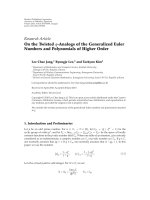
near the origin. Please see Figure 1. This example can be
generalized to a sum of any number of chirplets with
arbitrary parameters and proves for the general case that
the interference terms are located away from the origin
[46]. This observation holds important application for the
determination of the adaptive kernel to be discussed in the
next section.
2.3. Optimal Kernel Determinat ion. Equal density contours
for the autoterms of chirplets are defined mathematically
by ellipsoids. The direction and length of the principle axes
are functions of the chirp rate and the time spread. These
axes can be identified with a Radon transform. Analysis

of the Radon transform reveals information regarding the
monocomponent chirp rates (β)andtimespreads(α).
Recall that the chirplet components lie at the origin of the
ambiguity space while the interference terms are located away
from the origin. The Radon transform of ambiguity function
of a normalized chirplet can be expressed as
R
c

ρ = 0, θ

=

∞
−∞
A
c
(
Ω
1
, Ω
2
)
δ
(
Ω
1
cos θ + Ω
2
sin θ

)
dΩ
1
dΩ
2
= 2π

π
λ
(
θ
)
exp

−
[ω
0
−t
0
tan θ]
2
4λ
(
θ
)

,
(11)
where λ(θ)
= (β +tanθ)

2
/4α + α/4. Based on the superposi-
tion property, the Radon transform will show peaks at values
of θ corresponding to the axes orientations of each of the
ellipsoids. In order to exclude the effect of the interference
terms in the calculation, the Radon transform is carried out
4 EURASIP Journal on Advances in Signal Processing
0
1
2
3
4
5
6
0 5 10 15 20 25 30 35 40
Frequency (Hz)
Time (s)
(a)
0
0
Ω
2
Ω
1
(b)
0
10
20
30
40

50
60
70
80
90
100
−20 0 20 40 60 80 100 120 140 160 180
R (θ)
Degrees
(c)
0
0
Ω
2
Ω
1
(d)
0
1
2
3
4
5
6
0 5 10 15 20 25 30 35 40
Frequency (Hz)
Time (s)
(e)
0
1

2
3
4
5
6
0 5 10 15 20 25 30 35 40
Frequency (Hz)
Time (s)
(f)
Figure 1: (a) WVD of two chirplets (α
1
= 0.01,β
1
= 0.2,t
1
= 20.05,ω
1
= 32.08,α
2
= 0.01,β
2
= 0.025,t
1
= 20.05, and ω
2
= 24.06).
(b) Representation of chirplets in ambiguity space. Cross-terms are located between the chirplets in the WVD, while in ambiguity space
they are located away from the origin. (c) Radon transformation in the neighbourhood of the origin (ρ
= 0). (d) Optimal kernel in the
ambiguity space. (e) Resulting time-frequency representation. (f) Smoothed pseudo-Wigner-Ville distribution of the signal. Reduction in

energy localization is noticeable in this representation.
EURASIP Journal on Advances in Signal Processing 5
Frequency
Time
(a)
Frequency
Time
(b)
Frequency
Time
(c)
Frequency
Time
(d)
Frequency
Time
(e)
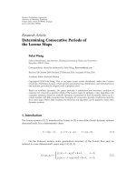
Figure 2: (a) Spectrogram of a frequency-modulated signal. (b) Wigner-Ville representation of the signal (negative energies discarded).
(c) Result of proposed method. (d) Choi-Williams representation of the signal. (e) Decomposition of signal in terms of seven
chirplets.
6 EURASIP Journal on Advances in Signal Processing
−0.3
−0.2
−0.1
0
0.1
0.2
00.511.52 2.53
Amplitude
Time (s)

×10
−3
(a)
0
1
2
3
4
5
6
7
×10
4
0123456
Frequency (Hz)
Time (s)
×10
−4
(b)
0
1
2
3
4
5
6
7
×10
4
00.511.522.5

Frequency (Hz)
Time (s)
×10
−3
(c)
0
1
2
3
4
5
6
7
×10
4
00.511.522.5
Frequency (Hz)
Time (s)
×10
−3
(d)
0
1
2
3
4
5
6
7
×10

4
00.511.522.5
Frequency (Hz)
Time (s)
×10
−3
(e)
Figure 3: Chirplet representations of a bioacoustical signal. (a) Time-domain representation of the large brown bat echo-location signal
(sampled at 0.14 MHz). (b) Spectrum of the signal (calculated with a 0.45 ms Gaussian window). (c) Time-frequency representation of the
signal. (d) Chirplet decomposition of the signal (represented by five chirplets). (e) Wigner-Ville distribution of the signal (negative energies
discarded).
EURASIP Journal on Advances in Signal Processing 7
Frequency
Time
(a)
Frequency
Time
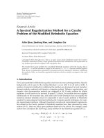
(b)
Figure 4: (a) Wigner-Ville distribution of a synthetic signal consisting of a sum of elementary signals [37]. (b) Resulting time-frequency
representation.
only in neighbourhood of the origin. This neighbourhood
is defined as the circular region around the origin which
includes 50% of the signal energy.
To eliminate artifacts due to sharp cutoffsfromker-
nel filtering (e.g., ringing), the edges of the kernel were
smoothed. The smoothing process can be carried out by
employing a tapering function like a Hanning or Gaussian
function. In Figure 1(d) we show the example of the use of a
two-dimensional Gaussian function. A “cleaned” ambiguity
representation is then obtained by multiplying the original

ambiguity function with the corresponding mask. Finally,
the time-frequency representation of the signal is generated
by calculating the inverse Fourier transform of the ambiguity
function.
If the signal of interest is not a sum of chirplets, the
steps outlined above will result in a representation where the
signal’s energy in the time-frequency plane is approximated
by a number of localized straight line segments. It should
be noted that for such signals, additional nonchirplet-
like interference terms will also appear. These interference
terms are often low frequency oscillations that overlap with
the signal in ambiguity space. For example, a frequency-
modulated signal and its Wigner Ville representation are
illustrated in Figure 2. Despite the nature of the signal, the
method proposed here can represent the signal in time-
frequency space with a high degree of localization. It can be
shown that the representation conserves 99% of the original
signal’s energy.
The Expectation-Maximization (EM) algorithm was
used for finding maximum likelihood estimation of chirplet
parameters in the time-frequency plane. All optimization
algorithms suffer from difficulties in parameter initialization
and in the selection of the number of parameters or
components. However, in this case we make use of the
parameters estimated from the Radon transformation in
ambiguity space. This significiantly reduces the time required
for optimization as well as improves the robustness of the
estimation. The number of components can also be set equal
to the number of peaks found in the Radon transformation,
and then adjusting the number of components from there to

minimize the total error.
3. Results and Discussion
Although biological signals can be found over a wide range of
frequencies, they are often narrowband in nature. Chirplets
are thus a suitable choice for modelling such signals [37].
The method proposed in this paper uses this property to
generate an interference-free time-frequency representation
by approximating the underlying time-frequency structures
of the signal by a linear approximation. The result provides
not only a clearer picture of the salient signal characteristics
but also provides a means for mathematically decomposing
signals into chirplets. An example of this is shown in
Figure 3, where a bat echo-location ultrasound signal is
represented as combination of four chirplets. We also show
results from synthetically generated signals—see Figure 4
where a signal consisting of a sinusoid, a windowed sinusoid,
Gabor logons, sawtooth, an impulse, and a chirplet is
analyzed by the same technique. This signal was adapted
from [37]. In both cases, the time-frequency visualization
is improved significantly and the main time-frequency
structures are easily identifiable.
We also provide one example where the time-frequency
representation is compared with that which was obtained
from chirplet decomposition with matching pursuit. Certain
dynamic brain mechanisms can be investigated through neu-
roelectrical brain responses called event-related potentials
(EPRs). The visual evoked potential (VEP) is an evoked brain
response generated in the visual cortex in response to the
presentation of a visual signal. Such signals are noisy and
are often averaged before processing. The VEP signal we

have analyzed here is equal to an average of 50 trails from a
single subject. Three chirplets are estimated for comparison
with the results calculated by Cui and Wong [37] using
the matching pursuit algorithm. As can be seen through
8 EURASIP Journal on Advances in Signal Processing
0
10
20
30
40
50
60
00.511.522.533.5
Frequency (Hz)
Time (s)
(a)
0
10
20
30
40
50
60
00.511.52 2.533.5
Frequency (Hz)
Time (s)
(b)
0
10
20

30
40
50
60
00.511.52 2.533.5
Frequency (Hz)
Time (s)
(c)
0
10
20
30
40
50
60
00.511.52 2.533.5
Frequency (Hz)
Time (s)
(d)
0
10
20
30
40
50
60
00.511.52 2.533.5
Frequency (Hz)
Time (s)
(e)

Figure 5: (a) Wigner-Ville distribution of visual evoked response (negative energies discarded). (b) Resulting signal representation after
applying optimal kernel. (c) Result obtained by Cui and Wong through chirplet decomposition via matching pursuit [37]. (d) Three chirplet
decomposition by the method proposed here. (e) Spectrogram of corresponding signal.
EURASIP Journal on Advances in Signal Processing 9
comparison of both figures, the results are quite similar. The
time-frequency representation was also verified through a
spectrogram.
A main challenge for chirplet decomposition is that
Gaussian chirplets do not form an orthogonal basis. One
solution is to employ suboptimal schemes like matching
pursuit. Figure 5 was generated by this particular approach.
While the underlying theory of matching pursuit is well
established, its numerical implementation in terms of
computational speed and accuracy comes at an enormous
cost. Matching pursuit requires that a large dictionary
of chirplet functions be generated in advance [47]. The
signal is decomposed iteratively by finding the best matched
dictionary component and then subtracted from the original
signal energy. This process continues until the residual
energy (error) becomes lower than a specified value. Finding
the best projection at each iterative step requires intensive
computational processing; maintaining a large dictionary
for good resolution and for long-enough signal lengths
involves steep storage requirements. In contrast, the method
proposed here does not rely on a dictionary and requires far
fewer computational steps. Note that chirplet decomposition
provides significant data compressibility. The VEP signal
shown in Figure 5 consisting of 480 samples can be well-
represented by as few as 15 parameters in terms of three
Gaussian chirplets.

Earlier it was shown that the cross-term interference
arising from a pair of monocomponents is located between
main components. Moreover, the interferences are oscilla-
tory in nature, and the spatial frequency of these oscillations
is a function of the distance between the components in
time and frequency. That is, the closer the two components,
the lower the oscillation frequency. In ambiguity space, this
would mean that the interference lies closer to the origin.
The low frequency interference also appears as a result of the
signal’s instantaneous frequency changing nonlinearly with
time. Due to the low frequency nature of these oscillations,
the cross-terms may not be completely removed by the kernel
due to overlap with signal components in the ambiguity
space. Although this interference can be removed at the post-
processing stage by (say) least-squares fitting to a Gaussian
density, it is important to remember that this interference
contributes to the signal’s overall energy distribution.
References
[1] T. Wang, J. Deng, and B. He, “Classifying EEG-based motor
imagery tasks by means of time-frequency synthesized spatial
patterns,” Clinical Neurophysiology, vol. 115, no. 12, pp. 2744–
2753, 2004.
[2] F. Miwakeichi, E. Mart
´
ınez-Montes, P. A. Vald
´
es-Sosa, N.
Nishiyama, H. Mizuhara, and Y. Yamaguchi, “Decomposing
EEG data into space-time-frequency components using Paral-
lel Factor Analysis,” NeuroImage, vol. 22, no. 3, pp. 1035–1045,

2004.
[3]B.Aysin,L.F.Chaparro,I.Grav
´
e, and V. Shusterman,
“Orthonormal-basis partitioning and time-frequency repre-
sentation of cardiac rhythm dynamics,” IEEE Transactions on
Biomedical Engineering, vol. 52, no. 5, pp. 878–889, 2005.
[4] R. Q. Quiroga and H. Garcia, “Single-trial event-related
potentials with wavelet denoising,” Clinical Neurophysiology,
vol. 114, no. 2, pp. 376–390, 2003.
[5]J.VanZaen,L.Uldry,C.Duch
ˆ
ene et al., “Adaptive tracking
of EEG oscillations,” Journal of Neuroscience Methods, vol. 186,
no. 1, pp. 97–106, 2010.
[6] H L. Liu, M L. Li, T C. Shih et al., “Instantaneous
frequency-based ultrasonic temperature estimation during
focused ultrasound thermal therapy,” Ultrasound in Medicine
and Biology, vol. 35, no. 10, pp. 1647–1661, 2009.
[7]E.Merlo,M.Pozzo,G.Antonutto,P.E.DiPrampero,
R. Merletti, and D. Farina, “Time-frequency analysis and
estimation of muscle fiber conduction velocity from surface
EMG signals during explosive dynamic contractions,” Journal
of Neurosc ience Methods, vol. 142, no. 2, pp. 267–274, 2005.
[8] G. Devuyst, J M. Vesin, P A. Despland, and J. Bogousslavsky,
“The matching pursuit: a new method of characterizing
microembolic signals?” Ultrasound in Medicine and Biology,
vol. 26, no. 6, pp. 1051–1056, 2000.
[9] L. Rankine, N. Stevenson, M. Mesbah, and B. Boashash, “A
nonstationary model of newborn EEG,” IEEE Transactions on

Biomedical Engineering, vol. 54, no. 1, pp. 19–28, 2007.
[10] P. Celka, B. Boashash, and P. Colditz, “Preprocessing and
time-frequency analysis of newborn EEG seizures,” IEEE
Engineering in Medicine and Biology Magazine, vol. 20, no. 5,
pp. 30–39, 2001.
[11] A. Monti, C. M
´
edigue, and L. Mangin, “Instantaneous param-
eter estimation in cardiovascular time series by harmonic
and time-frequency analysis,” IEEE Transactions on Biomedical
Engineering, vol. 49, no. 12 I, pp. 1547–1556, 2002.
[12] A. De Cheveign
´
e, “YIN, a fundamental frequency estimator
for speech and music,” The Journal of the Acoustical Society of
America, vol. 111, no. 4, pp. 1917–1930, 2002.
[13] P. Bonato, S. H. Roy, M. Knaflitz, and C. J. de Luca, “Time
frequency parameters of the surface myoelectric signal for
assessing muscle fatigue during cyclic dynamic contractions,”
IEEE Transactions on Biomedical Engineering,vol.48,no.7,pp.
745–753, 2001.
[14] I. Shafi, J. Ahmad, S. I. Shah, and F. M. Kashif, “Techniques
to obtain good resolution and concentrated time-frequency
distributions: a review,” EURASIP Journal on Advances in
Signal Processing, vol. 2009, 43 pages, 2009.
[15] D. Gabor, “Theory of communication,” Journal of the Institute
of Electrical Engineers, vol. 93, no. 26, pp. 429–457, 1946.
[16] J. B. Allen and L. R. Rabiner, “A unified approach to short-time
fourier analysis and synthesis,” Proceedings of the IEEE, vol. 65,
no. 11, pp. 1558–1564, 1977.

[17] W. Martin and P. Flandrin, “Wigner-ville spectral analysis
of nonstationary processes,” IEEE Transactions on Acoustics,
Speech, and Signal Processing, vol. 33, no. 6, pp. 1461–1470,
1985.
[18] L. Cohen, “Generalized phase-space distribution functions,”
Journal of Mathematical Physics, vol. 7, no. 5, pp. 781–786,
1966.
[19] E. Wigner, “On the quantum correction for thermodynamic
equilibrium,” Physical Review, vol. 40, no. 5, pp. 749–759,
1932.
[20] H. Margenau and R. N. Hill, “Correlation between measure-
ments in quantum theory,” Progress of Theoretical Physics,pp.
772–738, 1961.
[21] T. A. C. M. Claasen and W. F. G. Mecklenbrauker, “Wigner
distribution—a tool for time-frequency signal analysis,”
Philips Journal of Research, vol. 35, no. 4-5, pp. 276–300, 1980.
10 EURASIP Journal on Advances in Signal Processing
[22] P. Flandrin and W. Martin, “A general class of estimators
for the wigner-ville spectrum of nonstationary processes,” in
Systems Analysis and Optimization of Systems,LectureNotesin
Control and Information Sciences, pp. 15–23, Springer, Berlin,
Germany, 1984.
[23] R. D. Hippenstiel and P. M. de Oliveira, “Time-varying
spectral estimation using the instantaneous power spectrum
(IPS),” IEEE Transactions on Acoustics, Speech, and Signal
Processing, vol. 38, no. 10, pp. 1752–1759, 1990.
[24] M. Born and P. Jordan, “Zur Quantenmechanik,” Zeitschrift
f
¨
ur Physik, vol. 34, no. 1, pp. 858–888, 1925.

[25] H. Choi and W. J. Williams, “Improved time-frequency
representation of multicomponent signals using exponential
kernels,” IEEE Transactions on Acoustics, Speech, and Signal
Processing, vol. 37, no. 6, pp. 862–871, 1989.
[26] A. Papandreou and G. F. Boudreaux-Bartels, “Distributions
for time-frequency analysis: a generalization of Choi-Williams
and the Butterworth distribution,” in Proceedings of IEEE
International Conference on Acoustics, Speech, and Signal
Processing (ICASSP ’92), pp. 181–184, San Francisco, Calif,
USA, 1992.
[27] J. Jeong and W. J. Williams, “Kernel design for reduced inter-
ference distributions,” IEEE Transactions on Signal Processing,
vol. 40, no. 2, pp. 402–412, 1992.
[28] L. Cohen, “Distributions concentrated along the instanta-
neous frequency,” in Advanced Signal-Processing Algorithms,
Architectures, and Implementations, Proceedings of SPIE, pp.
149–157, July 1990.
[29] S. Kadambe, G. F. Boudreaux-Bartels, and P. Duvaut, “Win-
dow length selection for smoothing the Wigner distribution
by applying an adaptive filter technique,” in Proceedings of
IEEE International Conference on Acoustics, Speech, and Signal
Processing (ICASSP ’89), pp. 2226–2229, May 1989.
[30] D. L. Jones and R. G. Baraniuk, “Adaptive optimal-kernel
time-frequency representation,” IEEE Transactions on Signal
Processing, vol. 43, no. 10, pp. 2361–2371, 1995.
[31] J. C. Andrieux, M. R. Feix, G. Mourgues, P. Bertrand, B.
Izrar, and V. T. Nguyen, “Optimum smoothing of the wigner–
ville distribution,” IEEE Transactions on Acoustics, Speech, and
Signal Processing, vol. 35, no. 6, pp. 764–769, 1987.
[32] S. H. Doo, W S. Ra, T. S. Yoon, and J. B. Park, “Fast time-

frequency domain reflectometry based on the AR coefficient
estimation of a chirp signal,” in American Control Conference
(ACC ’09), pp. 3423–3428, June 2009.
[33] M. Jachan, G. Matz, and F. Hlawatsch, “Time-frequency
ARMA models and parameter estimators for underspread
nonstationary random processes,” IEEE Transactions on Signal
Processing, vol. 55, no. 9, pp. 4366–4381, 2007.
[34] N. Ma, D. Vray, P. Delachartre, and G. Gimenez, “Time-
frequency representation of multicomponent chirp signals,”
Signal Processing, vol. 56, no. 2, pp. 149–155, 1997.
[35] A. Akan, M. Yalcin, and L. Chaparro, “An iterative method
for instantaneous frequency estimation,” in Proceedings of the
8th IEEE International Conference on Electronics, Circuits and
Systems (ICECS ’01), vol. 3, pp. 1335–1338, 2001.
[36] M. Wang, A. K. Chan, and C. K. Chui, “Linear frequency-
modulated signal detection using radon-ambiguity trans-
form,” IEEE Transactions on Signal Processing,vol.46,no.3,
pp. 571–586, 1998.
[37] J. Cui and W. Wong, “The adaptive chirplet transform and
visual evoked potentials,” IEEE Transactions on Biomedical
Engineering, vol. 53, no. 7, pp. 1378–1384, 2006.
[38] N. Hess-Nielsen and M. V. Wickerhauser, “Wavelets and time-
frequency analysis,” Proceedings of the IEEE,vol.84,no.4,pp.
523–540, 1996.
[39] S. Mann and S. Haykin, “Chirplet transform: physical consid-
erations,” IEEE Transactions on Signal Processing, vol. 43, no.
11, pp. 2745–2761, 1995.
[40] S. Mallat, A Wavelet Tour of Signal Processing,TheSparseWay.
Academic Press, London, UK, 3rd edition, 2008.
[41] Y. Lu, R. Demirli, G. Cardoso, and J. Saniie, “A successive

parameter estimation algorithm for chirplet signal decompo-
sition,” IEEE Transactions on Ultrasonics, Ferroelectrics, and
Frequency C ontrol, vol. 53, no. 11, pp. 2121–2131, 2006.
[42] Y. Lu, R. Demirli, G. Cardoso, and J. Saniie, “Chirplet trans-
form for ultrasonic signal analysis and NDE applications,” in
IEEE Ultrasonics Symposium, pp. 536–539, September 2005.
[43] C. Ioana and A. Quinquis, “On the use of time-frequency
warping operators for analysis of marine-mammal signals,”
in Proceedings of IEEE International Conference on Acoustics,
Speech, and Signal Processing (ICASSP ’04), pp. 605–608, May
2004.
[44] Y. Tang, X. Luo, and Z. Yang, “Ocean clutter suppression
using one-class SVM,” in Proceedings of the 14th IEEE Signal
Processing Society Workshop on Machine Learning for Signal
Processing, pp. 559–568, October 2004.
[45] I.Shafi,J.Ahmad,S.I.Shah,andF.M.Kashif,“Computing
de-blurred time frequency distributions using artificial neural
networks,” Circuits, Systems, and Signal Processing, vol. 27, no.
3, pp. 277–294, 2008.
[46] P. Borgnat and P. Flandrin, “Time-frequency localization
from sparsity constraints,” in Proceedings of IEEE International
Conference on Acoustics, Speech, and Signal Processing (ICASSP
’08), pp. 3785–3788, April 2008.
[47] S. G. Mallat and Z. Zhang, “Matching pursuits with time-
frequency dictionaries,” IEEE Transactions on Signal Process-
ing, vol. 41, no. 12, pp. 3397–3415, 1993.