Báo cáo hóa học: " Research Article Network Modulation: An Algebraic Approach to Enhancing Network Data Persistence" doc

Hindawi Publishing Corporation
EURASIP Journal on Wireless Communications and Networking
Volume 2010, Article ID 141340, 15 pages
doi:10.1155/2010/141340
Research Article
Network Modulation: An Algebraic Approach to
Enhancing Network Data Persistence
Xiaoli Ma,
1
Giwan Choi,
1
and Wei Zhang
2
1
School of Electrical and Computer Engineering, Georgia Institute of Technology, Atlanta, GA 30332, USA
2
Qualcomm CDMA Technology, Qualcomm Inc., Santa Clara, CA 95054, USA
Correspondence should be addressed to Wei Zhang,
Received 2 January 2010; Revised 19 May 2010; Accepted 6 July 2010
Academic Editor: Xiaodai Dong
Copyright © 2010 Xiaoli Ma et al. This is an open access article distributed under the Creative Commons Attribution License,
which permits unrestricted use, distribution, and reproduction in any medium, provided the original work is properly cited.
Large-scale distributed systems such as sensor networks usually experience dynamic topology changes, data losses, and node
failures in various catastrophic or emergent environments. As such, maintaining data persistence in a scalable fashion has become
critical and essential for such systems. The existing major efforts such as coding, routing, and traditional modulation all have
their own limitations. In this work, we propose a novel network modulation (NeMo) approach to significantly improve the d ata
persistence. Built on algebraic number theory, NeMo operates at the level of modulated symbols (so-called “modulation over
modulation”). Its core notion is to mix data at intermediate network nodes and meanwhile guarantee the symbol recover y at
the sink(s) without prestoring or waiting for other symbols. In contrast to the traditional thought that n linearly independent
equations are needed to solve for n unknowns, NeMo opens a new regime to boost the convergence speed of achieving persistence.
Different performance criteria (e.g., modulation and demodulation complexity, convergence speed, finite-bit representation, and

noise robustness) have been evaluated in the comprehensive simulations and real experiments to show that the proposed approach
is efficient to enhance the network data persistence.
1. Introduction
Today large-scale distributed systems are routinely deployed
for many computing , detection, communication, and mon-
itoring tasks. These systems are comprised of a large
number of spatially distributed autonomous devices. Sensor
networks, cellular networks, Wi-Fi, computational grids,
data center, and peer-to-peer networks are among the typical
examples of this type of systems with broad practical appli-
cations in both civilian and military areas. It is ver y common
for these systems to incur data losses and node outages. For
instance, sensor nodes may be short-lived due to limited
energy resources or the failure in catastrophic/emergent
environments. Also because of nodes’ random placement,
network topology is unknown and the sink location(s) may
be unknown. Owing to all of these network uncertainties,
how to safely and soundly deliver the data to the sink(s)—
data persistence—becomes challenging and critical.
There are two major issues which have to be considered
and resolved for enhancing data p ersistence in a large-scale
distributed system. One is how to deliver the existing data to
the sink(s) as soon as possible.Thisisanimportantmetric
to evaluate the performance of an algorithm targeting data
persistence. Routing data to the sink(s) with the minimal
transmission overhead (e.g., delay) is a straightforward solu-
tion to this issue. However, existing routing protocols such
as [1–7] do not work appropriately due to lack of topology
information, or they have to pay high communication and
storage overhead when nodes are required to initiate data

reading and transmission immediately without learning the
network topology. The dynamics of network topology and
unexpected node failures make things even worse.
The other issue is concerned with how to “back-up” data
in the network so that if one node suddenly fails, its data
can still survive in other places of the network. One natural
approach is to adopt coding techniques. Recently, different
coding techniques have been proposed (e.g., [8–13]) to
increase data persistence. They show great improvement rel-
ative to the no coding case. However, there still exist several
unsolved problems. For example, some coding techniques
2 EURASIP Journal on Wireless Communications and Networking
require the sink to collect enough packets to decode the
next coded packet (see, e.g., [14]). This causes extra delay
and decoding complexity at the sink and may be impractical
for some applications with strict timeliness requirement
such as sensor networks for catastrophe monitoring. Also
the existing coding techniques are not flexible enough to
incorporate new node joins and/or asynchronous nodes.
In this work, we v iew these two issues from a new angle:
fast delivery can be interpreted as high transmission rate,
while robustness to node failure or noise can be viewed as
low error probability. This novel view makes enhancing data
persistence analogous to achieving Shannon’s capacity—
the maximum error-free data rate over a channel [15]. In
general, it is well known that there are two ways to achieve
Shannon’s capacity—coding and modulation. Recognizing
this, it is not surprising to see that coding techniques can
enhance data persistence. In addition, it becomes natural to
introduce our approach—modulation.

Traditionally, there are two major categories of mod-
ulation schemes—analog and digital modulations. Analog
modulation is applied continuously in response to the analog
information signal, for example, frequency modulation (FM)
for radio broadcasting. Clearly these modulation methods
are not capable of incorporating the distributed digital
data from sensors or other distributed autonomous devices.
Digitalmodulationisawaytogeneratewaveformsor
symbols f rom a digital bit stream, for example, phase shift
keying (PSK), quadrature amplitude modulation (QAM).
However, these traditional digital modulation schemes are
hard to “grow” when one node wants to combine two
symbols (not bits) to a new symbol in a higher constellation.
The symbols have to be demodulated back to bits and then
the union of two sets of bits is modulated to a new symbol.
Given the limited resources of a network node, this process
may cost infeasibly high energy and memory consumption.
In this paper, we propose a novel approach that is
referred to as network modulation (NeMo). NeMo is based
on algebraic number theory to enhance data persistence. This
approach adopts an algebraic way to “combine” symbols,
which increases the information in a symbol while still
guaranteeing the decodability at the sink. The core notion of
NeMo is to mix the data at intermediate network nodes while
allowing the sink to decode without prestored symbols.
Two different ways are proposed to modulate the
symbols—nonregenerative NeMo and regenerative NeMo.
They differ in the way that the newly received packet is
processed. In the nonregenerative version, a node simply
combines the incoming symbol with the local data. But the

regenerative version demodulates the arrived symbol before
combining it with the local data. Note that the modulation
and demodulation of NeMo operate at the level of modulated
symbols (called “modulation over modulation”) and thus
it can be independent from network layer. We formally
prove that for both of these methods the symbol recovery is
guaranteed at the sink and also carefully study all kinds of
performance tradeoffs of them. Furthermore, we derive the
upper bounds of the persistence curves with NeMo, which
illustrate that our approach is more efficient than the existing
Growth Codes (GCs) [13]. In addition, we propose solutions
to several pr actical concerns such as packet header design and
asynchronous node joins and failure.
The rest of this paper is organized as follows. We
summarize the related works in Section 2 and formulate
the problem and describe the network setting in Section 3.
Section 4 introduces the basics of NeMo and the modulation
and demodulation steps. Section 5 evaluates the perfor-
mance of NeMo. Implementation issues are addressed and
evaluated in Section 6. Section 7 presents the experiment
results. Section 8 concludes the paper and proposes some
future research directions.
2. Related Work
Distributed coding has been established as an effective
paradigm to deliver high data persistence in networked
systems. Like channel coding, its basic idea is to introduce
data redundancy to the network. The redundancy spread
over the network can help to recover the lost data in the
presence of noise and node failure. Some distributed coding
schemes have been developed for distributed storage systems

to provide the reliable access to the data [8, 9, 11, 12], and
for wireless sensor networks and peer-to-peer networks to
deliver significant improvement in throughput [16–21]and
reliability [13, 22–25]. Also, algebraic approach to network
coding was introduced in [26] and this frame was extended
to incorporate vector communication in linear deterministic
networks [27].
However, most of the techniques in this area require
accumulating a large number of codewords before decoding
by using the traditional coding techniques such as Reed-
Solomon [28], LT [29], Digital Fountain [14], LDPC [30],
and turbo codes [31]. This is not desirable in a number
of scenarios where resources are limited, nodes are subject
to failure at anytime, or a smooth data persistence curve is
required to provide low latency. In contrast, our NeMo can
perform decoding instantaneously after receiving the data.
Superposition coding is proposed to enhance the network
throughput in MAC layer [32] by taking into account
physical layer link information. However, symbol recovery
is needed at each node and the data persistence is not
considered.
Growth Codes (GCs) [13]isarecentmajoreffort to
maximize data persistence in a zero-configuration sensor
network. Nodes exchange codewords with their neighbors
while gradually increasing the codeword degree by combin-
ing received codewords with their own information. Liu et
al. [23] generalized the GC scenario to include multisnap-
shots and general coding schemes. By associating a utility
function with the recovered data, they design a joint coding
and scheduling scheme to maximize the expected utilit y

gain. Karande et al. [25] found that the random network
coding outperforms GC in periphery monitoring topologies.
Additionally, some other codes have been developed to
provide unequal protection for prioritized data. For example,
priority random linear codes [24] are proposed to partially
recover more important subset of data when the whole
recovery is impossible. Dimakis et al. [10] generalizes the GC
EURASIP Journal on Wireless Communications and Networking 3
analysis and investigates the design of fountain codes which
provide good intermediate performance and unequal error
protection for video streaming.
3. Problem Statement
In this section, for simplicity of illustration, we first present
a description of a simple network model we will use to
describe the design of NeMo. The model will be extended
for a number of practical issues later in this paper. Then we
define data persistence formally and formulate the problem
we attack in this work.
3.1. Network Description. Our network model is similar to
that considered in related works. It consists of a large sensor
network with N sensors/nodes and 1 sink. The network
is zero-configuration such that nodes only sense their
neighbors with whom they can communicate directly and do
not know where the sink is. The network topology is random
and can be altered. Typically the majority of the nodes cannot
communicate with the sink directly. In addition, our initial
study also makes the following assumptions:
(i) every node has infinite processing power and mem-
ory;
(ii) there is no node failure and data transmission error

(e.g., channel fading or additive noise);
(iii) each node takes only a single reading;
(iv) all data packets have the same importance;
(v) all nodes have the same transmission range;
(vi) every node employs the same modulation technique
and runs the same protocol;
(vii) all nodes have half-duplex capability, that is, trans-
mitting and receiving at different time slots (The
work in [13] assumes full-duplex capacity. However,
we believe half-duplex is more practical in the con-
text. O ur scheme also works for full-duplex scenario.)
The above assumptions construct a simple network
model which is most appropriate to show the design
principles and facilitate the analysis. Most of the assumptions
are also adopted in the literature (see, e.g., [6, 13, 21, 25]). We
will consider more practical network settings to address most
of the above unrealistic assumptions in Section 6.
3.2. Problem Formulation. Data per sistence is defined as the
fraction of data generated within the system that eventually
reaches the sink [13]. Now let us use a simple example to
illustrate what makes NeMo unique to enhance the data
persistence.
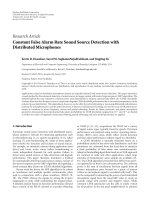
Example 1. Suppose that there are two nodes (Node 1 and
Node 2) with two readings/symbols, s
1
and s
2
for each.
The network is two-hop from Node 1 to Node 2 and then
to Sink (see Figure 1).Thegoalistodeliverboths

1
and
s
2
to the sink. Without combining s
1
and s
2
at Node 2,
3 hops are needed. We can do it in two hops if Node 2
Node 1 Node 2
SinkNode 1 Node 2
Sink
NeMo
s
1
s
1
s
1
s
2
x = f (s
1
, s
2
)
Traditional
Figure 1: A two-node example.
can transmit a combination of s

1
and s
2
, x = f (s
1
, s
2
),
in one slot. One question is: given two symbols, can we
find an efficient approach to combine them as one symbol
by guaranteeing identifiability at the sink side? For example,
for BPSK modulated symbols s
1
and s
2
, that is, s
1
, s
2
∈
{±
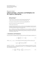
1}, when simple “adding” x = s
1
+ s
2
is applied, the
possible values of x (known as constellation) are shown in
the right subfigure of Figure 2. The (s
1
, s

2
) pair to generate
x is depicted under the corresponding point of x. From the
figure, it is ready to see that the unique recovery of original
readings is not guaranteed. For example, if x
= 0, the sink
does not know which pair among (0, 0), (
−1, 1), and (1, −1)
was sent from Node 1 and Node 2. However, if we “smartly”
combine s
1
and s
2
as x = s
1
+ e
jπ/4
s
2
, the constellation of x
is shown in the left subfigure of Figure 2. From the figure,
we can see that one unique x is designated to every pair of
s
1
and s
2
. That means when the sink receives x,itcaneasily
recover the original two symbols s
1
and s

2
. This shows that
if we combine two symbols “smartly,” symbol recovery is
guaranteed.
Mathematically, we formulate the problem as follows.
Suppose that s
2
is the local symbol at Node 2 and s
1
is a
symbol newly received at Node 2. After linear combination,
the symbol transmitted from this node to another node or
sink is
x
= λ
(
θ
1
s
1
+ θ
2
s
2
)
,
(1)
where λ is the power normalizer, and θ
1
and θ

2
are two
coefficients which are specified by modulation schemes. In
general, we have
x
= λ
D

n=1
θ
n
s
n
= λθs
T
,
(2)
where θ
= [θ
1
···θ
D
]ands = [s
1
···s
D
]. The remaining
question is how to choose
{θ
n

} so that {s
n
} can be uniquely
recovered from x. This may look like an ill-posed problem—
given one equation, how can one solve two or more
unknowns? The key is that
{s
n
} are not real or complex
numbers, but belong to some lattice (e.g., all QAM symbols
belong to complex Gaussian integer lattice). By appropriately
choosing
{θ
n
}, it can be guaranteed that {s
n
}will be uniquely
identified from x. We give the detailed design in the following
sections.
4. Design of NeMo
In this section, we briefly introduce algebraic number theory
and describe our NeMo design based on it.
4 EURASIP Journal on Wireless Communications and Networking
(0,1)
(0,
−1)
(1,0)
(
−1,0)
(1,1)

(
−1,−1)
(1,
−1)
(−1,1)
(0,0)
(0,1)
(0,
−1)
(1,0)
(
−1,0)
(1,1)
(
−1,−1) (1,−1)
(
−1,1)
(0,0)
Re
Im
Im
Re
Figure 2: Constellation at the sink in a two-node example.
4.1. Terminology and Notation. In the following, we summa-
rize some terminologies and corresponding notations which
will be used in the rest of the paper.
Symbol. We adopt s
k
’s to denote the originally modulated
symbols (before nodes exchange information), for example,

M-ary QAM. We call them OM symbols. Multiple OM
symbols can be modulated by NeMo into another symbol x
k
called an NM symbol.
Deg ree of an NM Symbol. The degree of an NM symbol x
is the number of OM symbols employed to generate this
symbol and is denoted as d.
Maximum Degree of an NM Symbol. Due to computational
power and memory size constraints, the degree of NM
symbols is usually upper bounded. The maximum degree
allowed is denoted as d
max
.
Neighbor. The nodes within the transmission range of a node
are called neighbors of this node.
Node ID. Node ID is a unique identity of a certain node in
the network. It can be an IP address, or a geographic location.
Symbol Overlap. If two NM symbols contain some common
OM symbols, we say these two symbols have some overlap.
Degree of a Modulator. It is defined as the length of the vector
as in (2) from which the coefficients θ
n
’s are drawn. W e will
see that the degree of a modulator is NOT always equal to the
degree of the corresponding NM symbol.
4.2. Algebraic Number Theory for NeMo. Before we pursue
the detailed modulation scheme, we need to introduce some
basics of algebraic number theory which will be used to
design NeMo.
Euler N umbers. GivenanintegerP, the Euler number φ(P)

of P is the cardinality of the set
{q :gcd(q, P) = 1, q ∈
[1, P)}, where gcd stands for the greatest common divisor.
As we mentioned, the key point of designing θ in (2)isto
make sure that when the OM symbols are linearly combined
as an NM symbol, they can still be uniquely demodulated.
There are different ways to design θ. Here we are providing
Table 1: Design of α = e
j2πq/P
.
D2345678910
P8916253649321850
a systematic and genera l way based on algebraic number
theory. For a given number of OM symbols D, the design
of has the following special structure
θ
=

1α ···α
D−1

,(3)
where α is a scalar which will be designed as follows. The
general design of α only depends on the modulator’s degree.
It does not depend on the original modulation size (say 4-
QAM or 16-QAM).
For a given modulator degree D, select an integer P which
is a multiple of D and φ(P)
= 2mD,wherem is a positive
integer. The generator α (and thus θ in (3)) can be designed

as
α
= e
j2πq/P
,
(4)
where q is selected from [1, P/D) such that gcd(q, P)
= 1,and
j
=
√
−1.
In the following, we provide one example to illustrate the
design of α.
Example 2. If D
= 2
k
, k ∈ N ∪{0}, then we can select P =
2
k+2
= 4D, and the Euler number φ(P) = 2D.Wecanchoose
q
= 1 such that gcd(q, P) = 1. Hence, α = e
j2π/P
.
Note that the choice of α is not unique. Different α
choices for the same size D may provide different perfor-
mance in physical layer (see, e.g., [33]), but all of them
achieve the same symbol identifiability. In Tabl e 1, we list the
design of α with some commonly used values of D. Although

the choice of q is nonunique, in the following, we adopt the
universal choice for all D,thatis,q
= 1.
4.3. The Basics of NeMo. Now we are ready to g o into the
design of NeMo. Note that, for simplicity we assume (i) each
packet sent by a node consists of a packet header which
includes the necessary information for network modulation
(see Section 6 for its design) and one NM/OM symbol as the
payload (the algorithm can be easily extended to multiple
symbols), and (ii) time is divided into rounds as in [ 13]. In
each round, a pair of nodes completes a packet exchange if no
EURASIP Journal on Wireless Communications and Networking 5
collision happens. The basic procedure is divided into three
stages and works as follows.
Initialization. Everynodehasonepacketreadyifany.
Exchange. In each round, each node tr ansmits its packet
with probability p.
(a) If a node decides to transmit the packet, it will
randomly select a neighbor to forward the packet.
The selected neighbor will receive the packet if it
does not transmit in the meanwhile (recall that we
assume half-duplex channel.). Otherwise the packet
is dropped and the rest of the round becomes idle.
Collision may also happen if a node is chosen for
exchange by more than one neighboring nodes at
the beginning of a round. Therefore, to summarize,
for one node to successfully receive a packet from
another node, three conditions must be met: (i)
this node decides not to transmit; (ii) it is selected
by another node to forward packets; and (iii) it is

not selected by more than one node (if collision is
considered).
(b) T hose nodes which successfully received packets will
forward their stored packets back to the correspond-
ing nodes to complete an exchange round.
Packet Processing. When a node receives a packet from its
neighbor, it will first check the packet header. If the packet
is completely new, that is, there is no overlap with the
node’s currently stored packet, the node will combine it into
the stored packet (i.e., network modulation). If the newly
received packet has some overlap with the stored one (judged
from the packet header), then the newly received packet will
be stored to replace the old one. In this case, the transmission
pair of two nodes just exchanges their packets.
It is not hard to see that exchanging may bring some
information loss if an old packet is replaced by the new one
even w hen the old one has new OM symbols. However, here
we consider a resource constrained environment (e.g., sensor
networks) so that intermediate nodes may not be able to afford
demodulating every NM symbol. We will discuss the variation
in Section 4.6 when nodes can afforduptoacertainlevel
of demodulation cost. If the node is the sink, then it will
demodulate the packet and save the data.
The aforementioned procedure works iteratively and
after some rounds the full data persistence wil l be achieved at
the sink. Next, we will describe how to process and modulate
incoming packets in detail.
4.4. Network Modulation. Suppose that a node has an NM
symbol x
1

of degree d
1
in the memory and receives a new
NM symbol x
2
of degree d
2
. The node will check the packet
header first for symbol overlap. If they have overlap, the
node’s old packet will be replaced by the new one. If they
have no overlap, the node will perform NeMo a s follows.
Case 1. If d
1
= d
2
= 1 (i.e., both are OM symbols), then the
modulation step is the same as the one in (2)withD
= 2.
Case 2. If d
1
or d
2
is greater than 1, we need to check the
degrees of modulator for x
1
and x
2
. Suppose that the degree
of the modulator of x
1

is D
1
and that of x
2
is D
2
≥ D
1
, the
new NM s ymbol is then generated as
x
= λ

α
1/2
2
x
1
+ x
2

,(5)
where α
2
is the generator of x
2
. After modulation, x becomes
an NM symbol with the degree of the modulator D
= 2D
2

,
but it only contains d
1
+ d
2
nonzero OM symbols.
The proof for the symbol recovery of nonregenerative
NeMo is given as follows. First, based on Cases 1 and 2,one
can verify that all NM symbols have θ’s size D
= 2
k
, k ∈
N ∪{
0}, recursively.
Second, based on Example 2 in Section 4.2, the generator
α for θ is e
j2π/P
and P = 2
k+2
provided D = 2
k
. Given two
degrees D
1
= 2
m
and D
2
= 2
n

,wherem ≤ n, x
1
and x
2
can
be represented as
x
1
=
d
1

k=1
α
k−1
1
s
1,k
,
x
2
=
d
2

k=1
α
k−1
2
s

2,k
=
d
2

k=1

α
1/2
2

2(k−1)
s
2,k
,
(6)
where α
1
= e
j2π/2
m+2
and α
2
= e
j2π/2
n+2
. Because we have
α
1/2
2

= e
j2π/2
n+3
,
α
1/2
2
x
1
=
d
1

k=1
e
j2π(2
n−m+1
(k−1)+1)/2
n+3
s
1,k
=
d
1

k=1

α
1/2
2


2
n−m+1
(k−1)+1
s
1,k
.
(7)
Combining (7)and(6), by defining a new generator as α
=
e
j2π/2
n+3
, we obtain that x actually is a linear combination
of x
1
and x
2
with modulator degree 2D
2
. According to
Example 2 in Section 4.2, this new α guar a ntees identifiabil-
ity. Note that the degree of the modulator is greater than the
degree of the NM symbol here.
Next, we will illustrate how the sink demodulates the
received packets to recover original OM symbols.
4.5. Network Demodulation. After explaining the modula-
tion schemes of NeMo, we now define the demodulation of
NeMo, that is, how to recover OM symbols from the received
NM symbols at the sink.

Let us define an important concept—the effective degree
of an NM symbol first. The set of demodulated OM symbols
stored at the sink is denoted as X.AnewlyreceivedNM
symbol x has degree d.Theeffective degree of x,denoted
by d
e
, is defined as the number of OM symbols that are
contained in x but not present in X. The node IDs of
associated OM symbols in x are contained in the packet
header of x (see Section 6), we can compute the effective
degree d
e
by simply comparing with the set X. Note that the
packet header stores all the necessary information so that the
6 EURASIP Journal on Wireless Communications and Networking
modulation coefficients θ
k
’s can be derived and the adopted
coefficients are known (see Section 6.1 for details).
The demodulation proceeds as follows.
(i) If d
e
= 0, the sink simply discards the packet with
NM symbol x since all the OM symbols contained in
x are known.
(ii) If d
e
= 1, the only unknown OM symbol can
be obtained by subtracting other demodulated OM
symbols from x.

(iii) If d
e
> 1, we first cancel the known OM symbols
from x and obtain an NM symbol modulated by
d
e
unknown symbols finally. Then, by exhaustively
searching over all possible d
e
× 1OMsymbolvectors
which have been saved in a look-up table, we can
determine the rest unknown OM symbols. Due to
the design of θ in Section 4.2,ad
e
× 1OMsymbol
vector can be uniquely determined given only one
NM symbol.
Note here, the demodulation of NeMo is different from
the decoder of the GC in [13]. Instead of discarding the
packets which contain more than one unknown symbol as in
GC, NeMo is able to demodulate any number of unknown
OM symbols through a look-up table. The demodulation
complexity of NeMo is mainly determined by searching the
look-up table. Suppose that the size of the constellation of
OM symbol is M. Then, the complexity of the exhaustive
search is O(M
d
e
). The constellation size for OM symbols is
typically small, for example, constellation size 2 (BPSK) and

4 (QPSK) are usually adopted. Therefore, the demodulation
complexity is mainly determined by the distribution of
the effective degree of received NM symbol. Later we will
use simulation to illustrate the distribution of the effective
degrees at the sink.
4.6. Regenerative NeMo. So far NeMo requires no demod-
ulationateachnode.Thus,inthefollowing,wenameit
nonregenerative NeMo. However, this may be too pessimistic
in some scenarios and cannot increase persistence “efficiently
and agg ressively” since it discards overlapping NM symbols
even when they contain new OM symbols. In the foll owing,
we propose a variation of NeMo, namely regenerative NeMo,
which is able to exploit the tradeoff between computational
resources and p erformance.
In contrast to nonregenerative NeMo, in regenerative
NeMo nodes will demodulate the NM symbol in each incom-
ing packet into OM symbols (the demodulation procedure is
the same as the one described in Section 4.5)andonlykeep
the ones which have not been stored at the node. Note that
here the nodes only store OM symbols. When a node decides
to exchange packets, it w ill modulate all the OM symbols it
stores into an NM symbol and send it to the randomly picked
neighbor as
x
= λ
⎛
⎝
d

k=1

θ
k
s
k
⎞
⎠
,(8)
where θ
k
is the kth entry of a vector with length d, λ is the
power normalizer, and s
k
’s are the selected OM symbols.
Note that the demodulation complexity is determined
by the degree of the NM symbols d. Therefore, a nonsink
node may not be able to afford demodulating NM symbols
with unbounded degrees and have to set a constraint on the
maximal degree (denoted by d
max
) of an NM symbol. With a
d
max
setting, the procedure of regenerative NeMo is modified
as follows.
Suppose that a node receives an NM symbol x with
effective degree d
e
and it has m (1 ≤ m ≤ d
max
)OMsymbols

stored (including the local reading).
(i) If d
e
>d
max
, the node will discard the arrival
since it does not have enough resource to afford
demodulation of x.
(ii) If d
e
= d
max
, the node demodulates x into d
e
new
OM symbols and then randomly replaces one OM
symbol among the d
e
OM symbols received with its
local reading. These d
max
OM symbols will be saved
in the memory and other symbols in the memory will
be discarded.
(iii) If d
e
<d
max
and d
e

+ m>d
max
, after demodulation,
the node will randomly pick d
max
− d
e
− 1symbols
from the m
−1 nonlocal OM sy mbols, and save them
with the local reading and d
e
newly received OM
symbols. The other OM sy mbols in the memory are
discarded.
(iv) Otherwise (d
e
+ m ≤ d
max
), the node just saves d
e
+ m
OM symbols in the memory.
In any case, the node only stores up to d
max
OM symbols
in its memory. Whenever there is a chance for transmission,
the node just modulates the OM symbols in its memory into
one NM symbol as in (8) and sends it out.
In summary, the general rules for regenerative NeMo

are: (i) giving the newly received OM symbols and local
reading higher priority to be stored and transmitted in the
next round so that the new data have more chances to be
circulated as soon as possible; and (ii) discarding the old OM
symbols in the memory in order to limit storage space usage
and search complexity.
We can further demodulate a subset of the incoming
NM symbols selectively (e.g., random selection or thresh-
olding on the degree of NM symbol) in order to achieve
different tradeoffs between computational complexity a nd
performance in different environments. In this sense, the
nonregenerative version can be viewed as a special case of
regenerative NeMo .
5. Performance Evaluations
We have introduced the proposed NeMo design with some
assumptions described in Section 3.1. In this section, we
adopt computer simulations to evaluate the performance of
NeMo. For the sake of comparison, the performance of the
GC in [13 ] is also provided.
EURASIP Journal on Wireless Communications and Networking 7
0 50 100 150 200
0
1
0.1
0.2
0.3
0.4
0.5
0.6
0.7

0.8
0.9
Number of exchange rounds
Data persistence
Optimal
Optimal, d
max
= 64
Optimal, d
max
= 8
Optimal, d
max
= 1
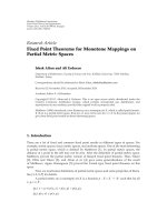
Figure 3: Optimal performance of NeMo with different d
max
.
5.1. Optimal Case. Letusfirstevaluatetheoptimalcases
for NeMo, that is, the upper bound of the persistence
performance. As shown in (5)and(8), NeMo combines two
NM symbols with degrees d
1
and d
2
to generate a new NM
symbol of degree d
1
+ d
2
. Each node aggressively increases

the degree of its NM symbol no matter nonregenerative
or regenerative NeMo is adopted. Suppose at the current
exchange round, all NM symbols at the nodes of the network
have degree d (or d OM symbols). Then after one exchange
round, the degree of all NM symbols will be increased to as
high as 2d when the new arrival contains completely new
symbols (denoted by optimal case). Assume at the beginning
(round 0), all nodes only have one OM symbol (or can
be seen as NM symbol of degree 1), the degree of all the
NM symbols will become 2
k
after k exchanges under the
optimal case. Therefore the maximal number of OM symbols
recovered at the sink after K exchange rounds is

K−1
k=0
2
k
=
2
K
− 1. Considering at most N OM symbols exist in an N-
node network, the upper bound of the persistence after K
rounds is thus min((2
K
− 1)/N,1).
If we bound the degree of NM symbols at each node by
d
max

, the upper bound on the persistence after K exchanges
becomes
min
⎛
⎝
2
log
2
d
max
+1
− 1+

K − 1 −

log
2
d
max

d
max
N
,1
⎞
⎠
.
(9)
In Figure 3, we plot the optimal persistence curves with
different d

max
for a network of N = 500 nodes. Different
from GC, the optimal persistence curves with d
max
can
increase faster than linear with slope 1/N.Forexample,when
d
max
= 2,thepersistencerateis(2K − 1)/N which increases
with slope 2/N.
200 400 600 800 1000
Non-reg NeMo, t
s
= 150
Non-reg NeMo, t
s
= 500
Reg NeMo, t
s
= 150
Reg NeMo, t
s
= 500
Reg NeMo, d
max
= 6, t
s
= 150
Reg NeMo, d
max

= 6, t
s
= 500
GC, scheduled sink, t
s
= 150
GC, scheduled sink, t
s
= 500
0
0
1
0.1
0.2
0.3
0.4
0.5
0.6
0.7
0.8
0.9
Number of exchange rounds
Data persistence
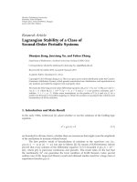
Figure 4: The effects of synchronousness.
The numerical evaluation setup for our NeMo tech-
nique is described as follows. The network is generated by
randomly distributing N
= 500 nodes in a 1 × 1square
area. One sink node is also randomly placed in the network
to collect the information but does not generate its own

reading. Differing from the related works [13, 22, 25], we
consider the sink as a normal node which does not send
out any packets. Since no node knows where the sink is, the
sink will not send out requests to its neighbors but simply
wait for random deliveries. The radius of the neighborhood
for each of these 501 nodes is R
= 0.3. BPSK modulation
is employed for OM symbols generated at each node. Also,
symmetric link is assumed between each pair of nodes
within the transmission range. On MAC layer, we adopt
slotted transmissions (i.e., the time is divided into exchange
rounds), and collisions are possible at each node but the
sink can resolve collisions. The probability that each node
transmits its packet at the beginning of each exchange round
is fixed as p
= 0.5.
Based on this network setup, we compare the data
persistence obtained by simulating our NeMo, GC, and
no coding on the network. No coding is a scheme in
which nodes exchange an OM symbol or a codeword
without any further modulation or coding. Because the
network is random and the packet forwarding is random,
the persistence actually is a random number. Therefore, we
illustrate the persistence in both average (as in all other
references) and outage performance which are important
to quantify the statistical property of persistence. More
than 100 realizations of the random network are simulated
to obtain the average persistence performance, while over
1500 realizations are simulated to depict outage persistence
curves.

8 EURASIP Journal on Wireless Communications and Networking
5.2. Average Persistence
Synchronization Issue. When the sensor nodes are deployed
in emergent scenarios, such as fires, floods, or earthquakes,
they must start collecting and transmitting data quickly,
having little chance to synchronize among themselves. Also
different sensors may get their readings at different times.
Thus, here we study the effects of synchronousness. For the
same simulation setup as Section 5.1, we set the starting
timeofeverynodetoberandomlyselectedfrom1tot
s
.
Figure 4 shows the persistence as a function of exchange
rounds for n onregenerative NeMo, regenerative NeMo (no
d
max
and d
max
= 6), and GC (with a scheduled sink) when
the nodes are not synchronized (t
s
= 500 and t
s
= 150).
We can see the performance of GC degrades dramatically
though we adopted “scheduled sink” as in [13]. Again, this is
because the optimal degree distribution, which is hard-coded
into the nodes before their deployment, cannot maximize
the decoding probability at the sink while the degree of a
codeword is increased. However, NeMo does not have any

requirement on synchronization and is much less affected by
the asynchronism.
Collision Effects. As in most related works such as [13, 22,
25], a full-duplex network with perfect collision resolution
is considered, for example, one node can exchange with
multiple nodes at the same time. Here, we use this full-duplex
scenario as a benchmark on the performance study. We plot
the data persistence of nonregenerative NeMo, regenerative
NeMo (no d
max
and d
max
= 6, 10), and the GC in Figure 5(a).
From the figure, we observe that the data persistence of GC
cannot reach one if the sink follows the same protocol as
a normal node (“GC, normal sink”). This is because the
sink is not always chosen by the neighbors to exchange
packets and thus the optimal degree distribution proposed
in [13] is violated. However, NeMo still reaches persistence
1 fast even with this normal sink. Even when GC performs
scheduling at the sink (“GC, scheduled sink”) as in [13],
NeMooutperformsGCwithmuchfasterconvergencespeed.
Regenerative NeMo converges faster than nonregenerative
NeMo because it more aggressively collects new symbols at
the expense of higher complexity. Regenerative NeMo with a
degree constraint d
max
= 6, 10 (with a normal sink), which
is more practical given resource constrained networks, also
performs much better than GC (with a normal sink) and no

coding scheme.
Now, we come back to the more practical setup—half-
duplex transmission with collision. Figure 5(b) compares
different schemes where collisions may happen in every
node (including sink). Compared with collision resolution
case, the persistence curves converge slower than the case in
Figure 5(a). NeMo is quite robust to collision. Usually, the
“perfect no collision” case in Figure 5(a) is too optimistic,
while the “collision at every node” case in Figure 5(b) is too
pessimistic. In Figure 5(c), we consider that only the sink is
capable to resolve collisions while other nodes cannot. Here,
we can see that NeMo performs similarly to the other two
cases and outperforms GC. In the following, we just adopt
this network setup unless otherwise mentioned.
5.3. Outage Analysis. To show the bandwidth efficiency of
our designs, we now investigate the outage performance.
The outage probability is defined as the probability that the
network persistence is less than a certain threshold. We consider
nonregenerative and regenerative NeMo, and plot the outage
probability versus exchange rounds in Figure 6 by fixing the
threshold persistence as 90%. We do not plot the outage
curve for GC because it cannot reach 90% persistence as we
can see in Figure 5(c). For the fixed threshold persistence,
the design represented by the curve on the left has better
outage performance than the one associated with the curve
on the right, since the left curve achieves zero outage
probability with fewer exchanges. From Figure 6, we find that
regenerative NeMo with d
max
= 10 has the worst outage

performance. This is because the NM symbol degrees are
limited by d
max
, and thus introduce a large “tail” in the pdf
of persistence. It is clear that regenerative NeMo (no d
max
)
achieves the best outage performance (i.e., decay fastest)
since the nodes decode received NM symbols and retain the
new information, while in nonregenerative NeMo some new
information will be dropped.
5.4. Complexity Analysis. Usually, network nodes (e.g., sen-
sors) have limited computing power. In NeMo, nodes need
to perform modulations and/or demodulations described
in Section 4. If the modulation/demodulation complexity is
high, the node may lack t imely response and be drained fast.
In this subsection, we analyze the complexity of modulation
and demodulation schemes at the sink and the other nodes.
The complexity is evaluated by counting the number of arith-
metic operations required for modulation/demodulation.
5.4.1. At the Sink. Effective degree is an important indicator
on the complexity of demodulation. We first plot the cdf of
the effective degrees of received NM symbols at the sink in
Figure 7(a).TheX-axis represents the effective degree and
Y-axis denotes the corresponding percentage of the received
symbols which have effective degrees less than or equal to
this degree. From the figure, we can see that the probability
to demodulate a symbol with high effective degree is really
low, since for most packets (>90% for nonregenerative NeMo
and >85% for regenerative NeMo) received at the sink the

degree is less than or equal to 5. The reason that regenerative
NeMo has higher effective degree than nonregenerative
NeMo is that regenerative NeMo increases the degree more
aggressively. Furthermore, we find that upper bounding the
degree of NM symbols by d
max
= 6 can further reduce
the percentage of high degrees. Therefore, we claim that the
complexity of demodulation scheme of NeMo is fairly low.
The sink node demodulates incoming packets and stores
the demodulated OM symbols in the memory. These OM
symbols are used to cancel the effect of known symbols
on the received NM symbol x of degree d to get a new
NM symbol x
e
of effective degree d
e
. This requires d − d
e
adding and multiplying operations. Then, we compare all
possible M
d
e
vectors with x
e
to find a unique symbol vector,
where M is a constellation size. For each comparison, the
sink performs d
e
adding and multiply ing operations. Thus,

EURASIP Journal on Wireless Communications and Networking 9
Non-reg NeMo
Reg NeMo
Reg NeMo, d
max
= 10
Reg NeMo, d
max
= 6
GC, normal sink
GC, scheduled sink
No coding
200 400 600 800 10000
0
1
0.1
0.2
0.3
0.4
0.5
0.6
0.7
0.8
0.9
Number of exchange rounds
Data persistence
(a)
200 400 600 800 10000
0
1

0.1
0.2
0.3
0.4
0.5
0.6
0.7
0.8
0.9
Number of exchange rounds
Data persistence
Non-reg NeMo
Reg NeMo
Reg NeMo, d
max
= 10
Reg NeMo, d
max
= 6
GC
(b)
200 400 600 800 10000
0
1
0.1
0.2
0.3
0.4
0.5
0.6

0.7
0.8
0.9
Number of exchange rounds
Data p
ersistence
Non-reg NeMo
Reg NeMo
Reg NeMo, d
max
= 10
Reg NeMo, d
max
= 6
GC
(c)
Figure 5: (a) Collisions are resolved at every node; (b) collisions happen at every node; (c) collisions happen at nodes except sink.
d
e
× M
d
e
+(d − d
e
) operations are needed to demodulate
one NM symbol at the sink. The demodulation complexity at
the sink for different d
max
when BPSK is employed is plotted
in Figure 7(b).Asd

max
becomes large, the sink receives
NM symbols with higher degree and hence the complexity
becomes higher due to exhaustive search for demodulation.
5.4.2. At the Other Nodes. Non-regenerative NeMo does not
require to demodulate at each node. The demodulation
complexity of regenerative NeMo is the same as that at
the sink. Typically, the normal nodes have less computing
resource than the sink so that they will have more limited
degree constraint.
Next we compare the modulation complexity for regen-
erative and nonregenerative NeMo. For regenerative NeMo,
the modulation complexity depends on the number of OM
symbols in the memory of the node. As shown in (8), d
multiplications and d
−1 additions are required to modulate
d OM symbols. For nonregenerative NeMo, suppose that
we want to modulate two NM symbols each of which is
of degree d
1
and d
2
, respectively. According to (5), the
node only needs 1 adding and multiplying operation no
10 EURASIP Journal on Wireless Communications and Networking
200 400 600 800 10000
Number of exchange rounds
10
−2
10

−1
10
0
Outage Probability (log scale)
Non-reg NeMo, 90%
Reg NeMo, 90%
Reg NeMo, d
max
= 10, 90%
Figure 6: Outage performance.
matter what d
1
and d
2
are. The node performs 1 additional
adding and multiplying operation when it adds its own
information. Figure 7(c) plots the complexity curves for both
regenerative and nonregenerative versions. We find they are
close to each other and climb up slowly with the increase
of d
max
. Figure 7(c) also includes a demodulation curve for
comparison. We can see that the complexity of modulation is
orders of magnitude smaller than that of demodulation. This
confirms the intuition that regenerative NeMo consumes
more computing resource and the NM degree needs to be
limited.
6. Implementation Issues
To this point, we have presented the NeMo under the ideal
case with the assumptions in Section 3.1. To implement

NeMoinarealnetwork,wehavetodealwithanumber
of limitations and requirements arisen from a resource-
constrained environment. In this section, we carefully inves-
tigate and evaluate the major implementation issues includ-
ing limited communication and storage usage, and node
failure, making NeMo feasible for real world applications.
6.1. Packet Overhead. As stated in Section 4,nodesexchange
packets with each other, and a packet includes a packet
header and an NM symbol as the payload. Since the
processing of received packets are different for regenerative
and nonregenerative NeMo, the corresponding design of the
packet header is also different.
For nonregenerative NeMo, to determine the coefficients
that are adopted to modulate the NM symbol, the packet
header must include the information to design the vector θ
in (3) and the positions of coefficients adopted, since not
all the elements of θ are used to modulate OM symbols.
Table 2: Average packet overhead (in bits).
N = 500 N = 1000
nonreg NeMo 704 1168
Reg NeMo 394 751
Reg NeMo (d
max
= 6) 64 71
GC (persistence 35%) 428 667
Because θ is uniquely determined by the modulator degree
D as shown in Section 4.2 and D is always selected as 2
k
for nonregenerative NeMo, we only need log
2

(log
2
D)bitsin
the header to determine D (and thus θ). To indicate which
elements of θ are used, we can put the indices of all the
adopted coefficients into the header, requiring dlog
2
D bits.
Notice that in this way we record the ordering information
of the used elements, which is important for demodulation
at the sink. Alternatively, we can have a D-bit bit-map to
indicate whether an element of θ is adopted (e.g ., “1” at the
nth bit means the nth element is adopted). But this way loses
the ordering information. The node ID overhead is the same
as the one in GC [13].
In general, the header design is not unique [13], we use
the first two bits of the header to signify which format is used
in this packet. Besides, we use the following 4 bits to represent
D,whichcansupportamaximumD as 2
16
− 1. The next
log
2
N bits (or log
2
d
max
bits if d
max
is set) are dedicated to

signify the degree of the packet.
For regenerative NeMo, we do not need to provide the
information of modulation coefficients, since the coefficients
are uniquely determined by the degree of the packet.
Therefore, only the node IDs are needed. So we only need
to record the sequence of the related source node IDs in the
packet header.
We simulate random networks in a 1
× 1squarearea
with the radius of the neighborhood of a node R
= 0.3and
compare the average length of packet headers for GC and
NeMo.TheaverageinbitsisprovidedinTable 2. For all the
schemes, the sink works as a normal node (not scheduled
sink) as we described before. The average packet overhead
for NeMo is obtained when persistence 1 is achieved, while
GC only achieves around 35% during the same time period.
From Table 2, we can see that for all the schemes, the
larger the network size, the longer the packet header. This
is due to the increase of symbols in the modulation/coding.
Among them the nonregenerative NeMo requires the longest
header because both the source node IDs and the coefficients
information need to be recorded. Furthermore, for the
regenerative NeMo, the d
max
setting suppresses the increase
of the packet overhead a lot since the number of both source
nodes and coefficients is upper bounded. We also find that
with d
max

= 6 the header does not increase much (from
64 to 71) when the network size is doubled. This is because
the length becomes same for every tr a nsmission after the
degree of an NM symbol reaches d
max
. Compared to GC,
our nonregenerative NeMo has longer packet header in the
time period of the simulation. However, considering the low
persistence rate and much longer time GC requires to achieve
EURASIP Journal on Wireless Communications and Networking 11
051015
65
70
75
80
85
90
95
100
e
Non-reg NeMo
Reg NeMo
Reg NeMo, d
max
= 6
(d
e
≤ e)(%)
(a)
0 5 10 15 20 25 30

10
3
10
4
10
5
10
6
10
7
10
8
10
9
d
max
Number of arithmetic operations
(log scale)
Non-reg NeMo
Reg NeMo
(b)
0 5 10 15 20 25 30
d
max
Number of arithmetic operations
(log scale)
10
0
10
2

10
4
10
6
10
8
Reg NeMo, demodulation complexity
Reg NeMo, modulation complexity
Non-reg NeMo, modulation complexity
(c)
Figure 7: (a) Distribution of the effective degrees; (b) complexity at the sink; (c) complexity at each node.
the persistence 1, the nonregenerative NeMo actually has the
less total overhead.
6.2. Waveform Storage and Noise Effect. To ma ke NeMo w or k
well in a resource-constrained system, memory usage is
an important issue. Usually the distributed devices (e.g., a
sensor) only have very limited memory space such that not
all the received information can be stored. In other words,
for practical implementation in a real network, we want the
memory usage to be as few as possible. In the following,
we discuss how the node stores its packet to maximize the
efficiency of memory usage.
For nonregenerative NeMo, besides the coefficient and
node ID information for constructing the packet header
(discussed in Section 4.1 ) when transmitting, we need to
store the NM symbol to be transmitted (as the payload).
As shown in (5), NM symbols are complex numbers so
that we need to apply finite bits with either floating-point
arithmetic or fixed-point arithmetic to represent them.
Although the precision is low, the fixed-point representation

is usually preferred because of its simplicity on hardware
implementation. Note that, no matter which representation
is adopted, quantization noise is introduced. Furthermore,
packet errors may be introduced and propagate in the
12 EURASIP Journal on Wireless Communications and Networking
0 100 200 300 400 500 600 700 800
0
0.02
0.04
0.06
0.08
0.12
0.1
Number of exchange rounds
Error rate of recovered OM symbo
ls
Non-reg NeMo d
max
= 6w/[4, 4]
Non-reg NeMo d
max
= 6w/[5, 5]
Non-reg NeMo d
max
= 6w/[6, 6]
Figure 8: Effect of finite-bit storage on NeMo.
network. We will show that only with a small number of bits,
the NeMo works very well numerically.
The network setup is the same as that in Section 5.
We adopt fixed-point arithmetics with G integer bits and

F fractional bits to store NM symbols in the memory.
Figure 8 depicts the error rate of recovered OM symbols at
the sink as a function of exchange rounds when d
max
=
6 for nonregenerative NeMo. Three curves are plotted for
(G, F) combinations (4, 4), (5, 5), and (6, 6), respectively. We
find that for (4, 4) and (5, 5) combinations, the error rate
increases quickly in the first a few rounds and keeps the same
level after that. This means the quantization error does not
deteriorate over time. We also find that with the increase of
memory usage, the error rate decreases dr amatically. When
the fixed-point representation with (6, 6) combination is
adopted, the performance is the same as that of the ideal case,
that is, no error happens at the sink. Similar claims hold for
regenerative NeMo .
Here, we reveal tradeoffs of NeMo on persistence rate,
memory usage, and complexity. If more bits are adopted,
the memory usage and complexity are higher, but persistence
rate is also higher. The trigger of these tradeoffsisd
max
. These
also show that NeMo is independent from physical layer
modulation once the waveforms are stored and operated as
bits. Therefore, the selection of d
max
should depend on the
network resources (e.g., complexity, delay constraint), but
not on the physical layer noise and link quality.
6.3. Node Failure. We want to make our scheme effective

and robust in a resource-constrained and disaster-prone
environment. Here we evaluate our NeMo in two types of
scenarios: (i) random failure, where every node randomly
dies due to the limited resource (e.g., battery power); and
(ii) regional failure, where the network or its par t s may be
0 100 200 300 400 500 600
Number of exchange rounds
Data persistence
Non-reg NeMo, t
r
= 100
Non-reg NeMo, t
r
= 20
Reg NeMo, t
r
= 100
Reg NeMo, t
r
= 20
Reg NeMo, d
max
= 6, t
r
= 100
Reg NeMo, d
max
= 6, t
r
= 20

0
1
0.2
0.4
0.6
0.8
(a)
0.15 0.2 0.25 0.3 0.35 0.4 0.45 0.5 0.55
0
1
0.2
0.4
0.6
0.8
Radius of disaster impact
Maximum persistence achieved
Non-reg NeMo, t
r
= 100
Non-reg NeMo, t
r
= 10
Reg NeMo, t
r
= 100
Reg NeMo, t
r
= 10
Reg NeMo, d
max

= 6, t
r
= 100
Reg NeMo, d
max
= 6, t
r
= 10
(b)
Figure 9: (a) Random failure when t
r
= 20 and 100; (b) Regional
failure when t
d
= 10 and 100.
destroyed or affected in some way. For example, in the event
of fire, flood, or earthquake, the nodes in a certain region
may stop functioning simultaneously.
6.3.1. Random Failure. Since transmissions consume much
more power than receptions we assume the battery energy
will be used up after a certain number of transmissions
(denoted by t
r
). The simulation setup is the same as that in
Section 5. t
r
is set to 20 and 100, respectively. The persistence
under this scenario is plotted in Figure 9(a). From the
figure, we can see that when t
r

= 100, the NeMo (both
EURASIP Journal on Wireless Communications and Networking 13
Reg NeMo
GC
200 400 600 800 10000
0
1
0.1
0.2
0.3
0.4
0.5
0.6
0.7
0.8
0.9
Number of exchange rounds
Data persistence
Non-reg NeMo
Figure 10: Average persistence from experiments.
Table 3: CPU time (in seconds).
Persistence 95% 35% 10%
Nonreg NeMo 55.07 3.55 0.84
Reg NeMo 38.77 4.76 1.65
GC N/A 1.5 0.25
nonregenerative and regenerative) is not impacted much
since they converge very fast (close to persistence 1 before 100
rounds). When t
r
= 20, the achieved persistence decreases

since a portion of symbols have not obtained the opportunit y
to propagate to the active areas. The d
max
constraint worsens
the performance.
6.3.2. Regional Failure. We simulate this scenario by dis-
abling part of the network a t the time of disaster. Suppose
that t
d
is the exchange round when the disaster happens, and
the nodes within distance r from a randomly located disaster
center will stop functioning and all the links connecting
them fail together. In Figure 9(b), we plot data persistence
as a function of the disaster radius r for t
d
= 10 and 100,
respectively. Similar to the observed in the random case,
when t
d
= 100, both regenerative and nonregenerative NeMo
(their curves are overlapped in the figure.) achieve the per fect
persistence regardless of the disaster radius due to the fast
convergence speed of NeMo. But if there is d
max
constraint,
the achieved persistence decreases when the disaster radius
increases. Again, we observe that more symbols are recovered
at the sink for a disaster that happened at t
d
= 100 than that

at t
d
= 10.
7. Experiment Results
We carry out an experiment with the software-defined
radio (SDR) to demonstrate the feasibility of NeMo in
practice. Both the transmitter and the receiver of SDR
are implemented by RFX2400 daughterboards as in [34],
which is a Universal Software Radio Peripheral (USRP) [35].
Channel coding is not applied in this experiment. Signal
processing modules such as modulation and demodulation
are implemented in Mat l a b . The square-root raised cosine
pulse shaping filter is adopted, and the symbol duration
is T
c
= 5T
e
,whereT
e
= 1 μs is the sampling period.
Complex samples are passed to the transmitter, where they
are converted to an analog signal by the dig ital to analog
converter, upconverted to the carrier frequency 2422 MHz,
and then transmitted through a wireless channel. This
process is inverted at the receiver.
For the network setup, 500 sensors/nodes and one sink
node are placed randomly in a 1
× 1squareareaasin
Section 5. The r adius of the neighborhood of each node
is R

= 0.3.TheOMsymbolsgeneratedateachnodeis
BPSK modulated as 1 or
−1. The slotted transmissions with
collisions are considered. The probability that each node
transmits its packet at the beginning of each exchange round
is fixed as 0.5. We set d
max
= 6 for both nonregenerative
and regenerative NeMo and assume that the sink operates
as a normal node. Here we also give nonregenerative NeMo
an upper bound on the modulation degree due to the
unavoidable noise effect in the real environment.
The communications among the 500 nodes are simulated
in Mat l a b, while the tr ansmission from one neighbor
(transmitter) to the sink (receiver) is implemented using
two RFX2400 daughterboards. The average persistence of
nonregenerative NeMo and regenerative NeMo is depicted in
Figure 10. The performance of GC is also given as a reference.
From the figure, we can see that both regenerative and non-
regenerative NeMo approach persistence 1 (even with d
max
=
6) in a practical environment quickly, while GC only collects
around 35% information. This confirms our observation
in simulation. We also compare the complexity of NeMo
andGCinTa ble 3 by measuring the CPU time required to
achieve persistence 95%, 35%, and 10%, respectively. Note
that the computational time to generate the network and
the neighbor list is not included. From the table we can
see that regenerative NeMo in general consumes more time

than nonregenerative NeMo because of the demodulation
complexity at each node. GC requires less time to achieve
low persistence thanks to its binary operations. As persistence
increases, GC becomes comparable with NeMo since NeMo
reaches higher persistence faster. In addition, GC never
reaches persistence higher than 35%.
8. Conclusion
In this paper, we have proposed a new approach—network
modulation (NeMo) to significantly enhance data persis-
tence for large-scale distributed systems. Based on algebraic
number theory, NeMo mixes data at intermediate network
nodes and meanwhile guarantees the symbol recovery at
the sink(s). In contrast to other existing methods, NeMo
works for asynchronous nodes in heterogeneous networks,
and also boosts data persistence over linear convergence
14 EURASIP Journal on Wireless Communications and Networking
speed. We have evaluated NeMo with different performance
criteria (such as modulation and demodulation complexity,
convergence speed, and memory usage). Both simulation
and experiment results show effectiveness of NeMo. NeMo
reveals a new regime for random network transmissions.
Some future research directions include enhancing network
lifetime by taking into account nodes with finite energy,
designing NeMo for nodes with unequal importance and/or
mobility, and investigating NeMo over wireless fading envi-
ronments.
References
[1] W. R. Heinzelman, J. Kulik, and H. Balakrishnan, “Adaptive
protocols for information dissemination in wireless sensor
networks,” in Proceedings of the 5th Annual ACM/IEEE

International Conference on Mobile Computing and Networking
(MOBICOM ’99), pp. 174–185, Seattle, Wash, USA, August
1999.
[2] J. N. Al-Karaki and A. E. Kamal, “Routing techniques in wire-
less sensor networks: a survey,” IEEE Wireless Communications,
vol. 11, no. 6, pp. 6–27, 2004.
[3] C. Perkins and P. Bhagwat, “Highly dynamic destination-
sequenced distance-vector routing (DSDV) for mobile com-
puters,” in Proceedings of the ACM Conference on Applica-
tions, Te chnologies, Architectures, and Protocols for Computer
Communication (SIGCOMM ’94), pp. 234–244, London, UK,
August-September 1994.
[4] D. Johnson and D. Maltz, “Dynamic source routing in ad-
hoc wireless networks,” in Proceedings of the ACM Conference
on Applications, Technologies, Architectures, and Protocols for
Computer Communication (SIGCOMM ’96), pp. 153–181,
Stanford, Calif, USA, August 1996.
[5] C. Perkins and E. M. Royer, “Ad-hoc on-demand distance
vector routing,” in Proceedings of the 2nd IEEE Workshop on
Mobile Computing Systems and Applications, pp. 90–100, New
Orleans, La, USA, February 1999.
[6] B. Karp and H. T. Kung , “GPSR: greedy perimeter stateless
routing for wireless networks,” in Proceedings of the 6th Annual
International Conference on Mobile Computing and Networking
(MOBICOM ’00), pp. 243–254, Boston, Mass, USA, August
2000.
[7] S. M. Das, H. Pucha, and Y. C. Hu, “MicroRouting: a
scalable and robust communication paradigm for sparse ad
hoc networks,” in Proceedings of the 19th IEEE International
Parallel and Distributed Processing Symposium (IPDPS ’05),

Denver, Colo, USA, April 2005.
[8] S.Acedanski,S.Deb,M.M
´
edard, and R. Koetter, “How good
is random linear coding based distributed networked storage?”
in Proceedings of the 1st Workshop on Network Coding, Theory,
and Applications, Riva del Garda, Italy, April 2005.
[9] A.G.Dimakis,P.B.Godfrey,M.J.Wainwright,andK.Ram-
chandran, “Network coding for distributed storage systems,”
in Proceedings of the 26th IEEE International Conference on
Computer Communications (INFOCOM ’07), pp. 2000–2008,
Anchorage, Alaska, USA, May 2007.
[10] A. G. Dimakis, J. Wang, and K. Ramchandran, “Unequal
growth codes: intermediate performance and unequal error
protection for v ideo streaming,” in Proceedings of the IEEE
Workshop on Multimedia Signal Processing, pp. 107–110,
Chania, Greece, October 2007.
[11] A. G. Dimakis, V. Prabhakaran, and K. Ramchandran, “Ubiq-
uitous access to distributed data in large-scale sensor networks
through decentralized erasure codes,” in Proceedings of the 4th
International Symposium on Information Processing in Sensor
Networks (IPSN ’05), pp. 111–117, Los Angeles, Calif, USA,
April 2005.
[12] A. Jiang, “Network coding for joint storage and transmission
with minimum cost,” in Proceedings of the IEEE International
Symposium on Information Theory (ISIT ’06), pp. 1359–1363,
Seattle, Wash, USA, July 2006.
[13] A. Kamra, V. Misra, J. Feldman, and D. Rubenstein, “Growth
codes: maximizing sensor network data persistence,” in Pro-
ceedings of the ACM Conference on Applications, Technologies,

Architectures, and Protocols for Computer Communication
(SIGCOMM ’06), pp. 255–266, Pisa, Italy, September 2006.
[14] J. W. Byers, M. Luby, M. Mitzenmacher, and A. Rege, “A digital
fountain approach to reliable distribution of bulk data,” in
Proceedings of the ACM Conference on Applications, Technolo-
gies, Architectures, and Protocols for Computer Communication
(SIGCOMM ’98), pp. 56–67, Vancouver, Canada, August-
September 1998.
[15] C. E. Shannon, “A mathematical theory of communication,”
Bell System Technical Journal, vol. 27, pp. 379–423, 623–656,
1948.
[16] R. Ahlswede, N. Cai, S Y. R. Li, and R. W. Yeung, “Network
information flow,” IEEE Transactions on Information Theory,
vol. 46, no. 4, pp. 1204–1216, 2000.
[17] S Y. R. Li, R. W. Yeung, and N. Cai, “Linear network coding,”
IEEE Transactions on Information Theory,vol.49,no.2,pp.
371–381, 2003.
[18] T.Ho,R.Koetter,M.M
´
edard, D. Karger, and M. Effros, “The
benefits of coding over routing in a randomized setting,” in
Proceedings of IEEE International Symposium on Information
Theory (ISIT ’03), pp. 227–234, Yokohama, Japan, June-July
2003.
[19] D. Wang, Q. Zhang, and J. Liu, “Partial network coding: theory
and application for continuous sensor data collection,” in
Proceedings of the 14th IEEE International Workshop on Quality
of Service (IWQoS ’06), pp. 93–101, New Haven, Conn, USA,
June 2006.
[20] S. Katti, D. Katabi, W. Hu, H. Rahul, and M. M

´
edard,
“The importance of being opportunistic: practical network
coding for wireless environments,” in Proceedings of the
Annual Allerton Conference on Communication, Control, and
Computing, Allerton, Ill, USA, September 2005.
[21] S. Katti, H. Rahul, W. Hu, D. Katabi, M. M
´
edard, and
J. Crowcroft, “XORs in the air: practical wireless network
coding,” in Proceedings of the ACM Conference on Applica-
tions, Te chnologies, Architectures, and Protocols for Computer
Communication (SIGCOMM ’06), pp. 243–254, Pisa, Italy,
September 2006.
[22] D. Munaretto, J. Widmer, M. Rossi, and M. Zorzi, “Network
coding strategies for data persistence in static and mobile
sensor networks,” in Proceedings of the International Workshop
on Wireless Networks: Communication, Cooperation and Com-
petition, pp. 1–8, Limassol, Cyprus, April 2007.
[23] J. Liu, Z. Liu, D. Towsley, and C. H. Xia, “Maximizing the data
utility of a data archiving & querying system through joint
coding and scheduling,” in Proceedings of the 6th International
Symposium on Information Processing in Sensor Networks
(IPSN ’07), pp. 244–253, Cambridge, Mass, USA, April 2007.
[24] Y. Lin, B. Li, and B. Liang, “Differentiated data persistence
with priority random linear codes,” in Proceedings of the IEEE
EURASIP Journal on Wireless Communications and Networking 15
International Conference on Distributed Computing Systems
(ICDCS ’07), pp. 47–47, Toronto, Canada, June 2007.
[25] S. Karande, K. Misra, and H. Radha, “Natural growth

codes: partial recovery under random network coding,” in
Proceedings of the 42nd Annual Conference on Information
Sciences and Systems (CISS ’08), pp. 540–544, Princeton, NJ,
USA, March 2008.
[26] R. Koetter and M. M
´
edard, “An algebraic approach to network
coding,” IEEE/ACM Transactions on Networking, vol. 11, no. 5,
pp. 782–795, 2003.
[27] J. Ebrahimi and C. Fragouli, “Algebraic algorithms for vec-
tor network coding,” 2010, fl.ch/record/
144144.
[28] S. B. Wicker, Reed-Solomon Codes and Their Applications, IEEE
Press, Piscataway, NJ, USA, 1994.
[29] M. Luby, “LT codes,” in Proceedings of the IEEE Symposium on
the Foundations of Computer Science (FOCS ’02), pp. 271–271,
Vancouver, Canada, November 2002.
[30] R. G. Gallager, “Low-density parity-check codes,” IEEE Trans-
actions on Information Theory, vol. 8, no. 1, pp. 21–28, 1962.
[31] C. Berrou, A. Glavieux, and P. Thitimajshima, “Near Shannon
limit error-correcting coding and encoding: turbo-codes,” in
Proceedings of the IEEE International Conference on Commu-
nications (ICC ’93), pp. 1064–1070, Geneva, Switzerland, May
1993.
[32] L. Li, R. Alimi, R. Ramjee et al., “Superposition coding for
wireless mesh networks,” in Proceedings of the 13th Annual
ACM Internat ional Conference on Mobile Computing and
Networking (MobiCom ’07), pp. 330–333, Montreal, Canada,
September 2007.
[33] Y. Xin, Z. Wang, and G. B. Giannakis, “Space-time diversity

systems based on linear constellation precoding,” IEEE Trans-
actions on Wireless Communications, vol. 2, no. 2, pp. 294–309,
2003.
[34] S. Katti, S. Gollakota, and D. Katabi, “Embracing wireless
interference: analog network coding,” in Proceedings of the
ACM Conference on Applications, Technologies, Architectures,
and Protocols for Computer Communication (SIGCOMM ’07),
pp. 397–408, Kyoto, Japan, August 2007.
[35] Ettus Research LLC, “Universal software radio peripheral,”
.