Báo cáo hóa học: "Research Article Efficient Vector-Based Forwarding for Underwater Sensor Networks" ppt

Hindawi Publishing Corporation
EURASIP Journal on Wireless Communications and Networking
Volume 2010, Article ID 195910, 13 pages
doi:10.1155/2010/195910
Research Article
Efficient Vector-Based Forwarding for
Underwater Sensor Networks
Peng Xie,
1
Zhong Zhou,
2
Nicolas Nicolaou,
2
Andrew See,
2
Jun-Hong Cui,
2
and Zhijie Shi
2
1
Intelligent Automation, Inc., Rockville, MD 20855, USA
2
Computer Science & Engineering Depart ment, Unive rsity of Connecticut, Storrs, CT 06269, USA
Correspondence should be addressed to Jun-Hong Cui,
Received 15 December 2009; Accepted 25 February 2010
Academic Editor: Qilian Liang
Copyright © 2010 Peng Xie et al. This is an open access article distributed under the Creative Commons Attribution License, which
permits unrestricted use, distribution, and reproduction in any medium, provided the original work is properly cited.
Underwater Sensor Networks (UWSNs) are significantly different from terrestrial sensor networks in the following aspects: low
bandwidth, high latency, node mobility, high error probability, and 3-dimensional space. These new features bring many challenges
to the network protocol design of UWSNs. In this paper, we tackle one fundamental problem in UWSNs: robust, scalable, and

energy efficient routing. We propose vector-based forwarding (VBF), a geographic routing protocol. In VBF, the forwarding path
is guided by a vector from the source to the target, no state information is required on the sensor nodes, and only a small fraction
of the nodes is involved in routing. To improve the robustness, packets are forwarded in redundant and interleaved paths. Further,
a localized and distributed self-adaptation algorithm allows the nodes to reduce energy consumption by discarding redundant
packets. VBF performs well in dense networks. For sparse networks, we propose a hop-by-hop vector-based forwarding (HH-
VBF) protocol, which adapts the vector-based approach at every hop. We evaluate the performance of VBF and HH-VBF through
extensive simulations. The simulation results show that VBF achieves high packet delivery ratio and energy efficiency in dense
networks and HH-VBF has high packet delivery ratio even in sparse networks.
1. Introduction
Recently, underwater sensor networks have emerged as a
very powerful technique for many applications in under-
water environments, including monitoring, measurement,
surveillance, and control [1–7]. Compared with traditional
techniques in these application scenarios, underwater sensor
networks enable people to perform underwater activities
more accurately and timely in much wider areas.
Even though underwater sensor networks (UWSNs)
share some common properties with terrestrial sensor net-
works, such as the large number of nodes and the limited
energy supplies, UWSNs are significantly different from
terrestrial sensor networks in many aspects: low bandwidth,
high latency, node mobility (resulting in high network
dynamics), high error probability, and three-dimensional
network topology. These new features bring many challenges
to the protocol design of UWSNs. In this paper, we tackle
one fundamental problem in UWSNs: robust, scalable, and
energy efficient routing. The unique features of UWSNs pose
great challenges on its routing protocol design and make
many existing routing protocols for terrestrial networks
unsuitable.

1.1. Unique Features of UWSNs. UWSNs are significantly
different from any terrestrial sensor networks in terms of the
following aspects.
(i) Low Bandwidth and High Latency in UWSNs.
Acoustic channels (instead of RF channels) are used
as the communication method since radio does not
work well in water. The propagation speed of acoustic
signals in water is about 1.5
× 10
3
m/sec, which
is five orders of magnitude lower than the radio
propagation speed (3
× 10
8
m/sec). Moreover, the
available bandwidth of underwater acoustic chan-
nels is limited and dramatically depends on both
transmission range and frequency. According to [8],
nearly no research and commercial system can exceed
2 EURASIP Journal on Wireless Communications and Networking
40 km
×kbps as the maximum attainable Range×Rate
product.
(ii) UWSNs Are Highly Dynamic. The underwater sen-
sor networks we target are highly mobile networks
where sensor nodes are not fixed and they will float
with water currents. From empirical observations,
underwater objects may move at the speed of 2-
3 knots (or 3–6 kilometers per hour) in a typical

underwater condition [6, 7]. This kind of mobility
results in a highly dynamic network topology.
(iii) UWSNs Are Highly Error-Prone.Underwateracous-
tic communication channels are significantly affected
by many factors such as signal attenuation, noise,
multipath, Doppler spread, and even water temper-
ature. All these factors cause high bit-error and delay
variance. Thus, communication links in UWSNs are
highly error-prone. Moreover, sensor nodes are more
vulnerable in harsh underwater environments. Com-
pared with their terrestrial counterparts, underwater
sensor networks have a higher node-failure rate and
packet-loss probability.
(iv) UWSNs Are Three-Dimensional. UWSNs are usu-
ally deployed in a three-dimensional space. This is
different from the 2-dimensional deployment of most
terrestrial sensor networks.
These characteristics of UWSNs bring up many new
challenges and make the existing routing protocols for
terrestrial sensor networks unsuitable here. For UWSNs, the
routing protocols should be able to handle the node mobility
and the unreliable communication links with high energy
efficiency.
1.2. Routing Challenges in UWSNs. UWSNs are highly
dynamic networks, which makes existing routing protocols
for stationary or quasistationary networks unsuitable. In
UWSNs, the mobility speed of nodes is around 1–3 meter
per second, the acoustic signal propagate at 1500 meter/s,
and the transmission range of the sensor nodes is less than
1 km. The low propagation speed of the acoustic signal and

relatively highly mobile nodes cause the network topology
change dramatically and dynamically. For example, when
the distance between the sender and the receiver is large,
it is possible that the network topology changes during
the time the data packet traverses the networks. Many
existing protocols for terrestrial networks are for relatively
stable network topology. Generally, these protocols fall into
two categories: proactive routing and reactive routing. In
proactive routing protocols such as OLSR [9], TBRPE [10],
andDSDV[11], routes need to be found and maintained
prehand, which is quite expensive for UWSNs. On the
other hand, in reactive protocols such as AODV [12]and
DSR [13], the route discovery process is triggered by the
communication demand at sources. In the phase of route
discovery, the source seeks to establish a route toward the
destination by flooding a route request message, which
would be very costly in dynamic networks. Thus, these
protocols are not suitable for UWSNs.
In UWSNs, nodes are usually powered by battery; thus
energy efficiency is one of the major design concerns. Many
energy efficient routing protocols for the terrestrial sensor
networks, such as Directed Diffusion [14], Two-Tier-Data
Dissemination (TTDD) [15], and GRAB [16], can not
be applied in UWSN since they are mainly designed for
stationary networks. Not much work has been done on the
energy efficient routing protocols for such highly dynamic
networks as UWSNs.
In addition, the unstable acoustic channel condition
and the dynamic network topology of UWSNs make the
conventional single path forwarding protocols very unre-

liable. Multipath routing [17, 18] which uses multiple
paths simultaneously for data transmission is a promising
technology here.
1.3. Contributions. We propose a novel routing protocol,
called vector-based forwarding (VBF), to address the routing
problem in UWSNs. VBF is an essentially geographic routing
protocol, which is robust, scalable, and energy efficient. In
VBF, the forwarding path is the vector from the source to
the destination. No state information is required on the
sensor nodes and only a small fraction of the nodes in
the networks are involved in routing. Moreover, packets are
forwarded along redundant and interleaved paths from the
source to the destination; it is robust against packet loss
and node failure. To enhance the performance of VBF in
sparse networks, we propose a variant of VBF, called hop-
by-hop VBF (HH-VBF). In HH-VBF, the forwarding path
is the vector from forwarding nodes to the target instead of
the one from the source to the target. HH-VBF is capable
of finding a forwarding path even in a very sparse network.
Further, we develop localized and distributed self-adaptation
algorithms to improve the performance of VBF and HH-
VBF. The self-adaptation algorithms allow the nodes to
weigh the benefit to forward packets and reduce energy
consumption by discarding low benefit packets. We evaluate
the performance of VBF and HH-VBF through extensive
simulations.
The rest of this paper is organized as follows. We first
briefly review some related work in Section 2.Then,we
present our VBF and HH-VBF protocol in Section 3.After
that, we evaluate VBF and HH-VBF through simulations in

Section 4. Finally, we conclude the paper in Section 5.
2. Related Work
In this section, we will review related work in both terrestrial
networks and underwater networks.
2.1. Routing in Terrestrial Wireless Networks. Energy effi-
ciency has long been recognized as one of the most important
properties for terrestrial wireless networks. Many energy
efficient routing protocols such as Directed Diffusion [14],
Two-Tier Data Dissemination [15], GRAdient [16], Rumor
routing [19], and SPIN [20], which aim for high energy
efficiency, have been proposed in the last few years for
terrestrial wireless networks. These protocols can achieve
EURASIP Journal on Wireless Communications and Networking 3
high energy efficiency in the terrestrial networks. However,
they depend on the relatively stable neighborhood to form
the routing path. If applying these protocols in UWSNs,
it would be costly to maintain and recover the frequently
broken routing path due to the node mobility.
Geographic routing protocols, which leverage the posi-
tion information of each node to determine the forwarding
path, have been investigated extensively for terrestrial wire-
less networks [21–26]. In [21], GPSR protocol, which always
selects the node geographically closest to the destination
of the target, is proposed. If GPSR cannot find any node
closer to the destination of the packet than the forwarder,
it adopts right-hand rule to forward the packet. Beacon-less
routing algorithm (BLR) in [22] selects the next hop through
Dynamic Forwarding Delay (DFD). Upon receiving a packet,
each node computes its DFD value determined by its posi-
tion. The node with the least DFD value forwards the packet.

The Contention-based forwarding (CBF) protocol proposed
in [23] selects the next hop by area-based suppression. In
CBF, only nodes in an area called suppression area contend
to forward the packet. The routing protocols proposed in
[24, 25] take not only the position but also the quality of the
link into consideration in selection of the next hop.
Since geographic routing protocols do not rely on the
stable neighborhood to find the forwarding path, it is a
very promising technique to address the routing issues
in networks with dynamic topology. Our proposed VBF
protocol is a kind of geographic routing protocols which is
adapted to the unique underwater environment.
2.2. Routing in Underwate r Networks. Much research work
has been done in the last few years on the routing protocols
for underwater networks. The challenges and state-of-art
for the routing protocols in underwater networks have been
discussedindetailin[5, 6]. A pioneering work is done in
[27] on the routing protocol for underwater networks. In
this work, a central master node is used to probe the network
topology and do the route establishment. The authors of [28]
propose a centralized routing algorithm for delay sensitive
application and a distributed routing algorithm for delay-
insensitive applications in three-dimensional underwater
networks. In [29], the authors propose a novel method to
improve the efficiency of the flood-based routing protocol
in underwater sensor networks. Focus beam routing appears
in [30], which dynamically establishes a route as the data
packet traverses the network towards its final destinations.
An adaptive routing protocol for underwater Delay Tolerant
Networks (DTN) has been proposed in [31], which divides

the network into multiple layers and every node adaptively
finds its routes to the upper layer according to its past
memory.
Different from all the above work, our VBF takes
advantages of the location information to form one or
multiple routing pipes from the source to the destination.
Multiple routes might be used simultaneously in VBF to
improve the reliability. At the same time, the self-adaption
algorithm in VBF can greatly improve the energy efficiency.
Thus, our VBF can achieve a good balance between the
reliability and energy efficiency.
3. Vector-Based Forwarding Protocol (VBF)
In this section, we present our vector-based forwarding
(VBF) protocol and its enhanced version, hop-by-hop
vector-based forwarding (HH-VBF) protocol in details.
3.1. Overview of VBF. In sensor networks, energy constraint
is a crucial factor since sensor nodes usually run on battery,
and it is impossible or difficult to recharge them in most
application scenarios. In underwater sensor networks, in
addition to energy saving, the routing algorithms should be
able to handle node mobility in an efficient way.
Vector-Based Forwarding (VBF) protocol meets these
requirements successfully. We assume that each node in VBF
knows its position information, which is provided by some
location algorithms [32–37]. If there is no such localization
service available, a sensor node can still estimate its relative
position to the forwarding node by measuring its distance to
the forwarder and the angle of arrival (AOA) and strength of
the signal by being armed with some hardware device. This
assumption is justified by the fact that acoustic directional

antennae are of much smaller size than RF directional
antennae due to the extremely small wavelength of sound.
Moreover, underwater sensor nodes are usually larger than
land-based sensors, and they have room for such devices. In
this work, we assume that the position information can be
calculated by measuring the AOA and strength of the signal.
In VBF, each packet carries the positions of the sender,
the target, and the forwarder (i.e., the node which transmits
this packet). The forwarding path is specified by the routing
vector from the sender to the target. Upon receiving a
packet, a node computes its relative position to the forwarder.
Recursively, all the nodes receiving the packet compute their
positions. If a node determines that it is sufficiently close
to the routing vector (e.g., less than a predefined distance
threshold), it puts its own computed position in the packet
and continues forwarding the packet; otherwise, it simply
discards the packet. In this way, all the packet forwarders in
the sensor network form a “routing pipe”: the sensor nodes
in this pipe are eligible for packet forwarding, and those
which are not close to the routing vector (i.e., the axis of
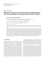
the pipe) do not forward. Figure 1 illustrates the basic idea
of VBF. In the figure, node S
1
is the source, and node S
0
is
the sink. The routing vector is specified by
−−→
S
1

S
0
.Datapackets
are forwarded from S
1
to S
0
. Forwarders along the routing
vector form a routing pipe with a precontrolled radius (i.e.,
the distance threshold, denoted by W in this paper).
As we can see, like all other source routing protocols, VBF
requires no state information at each node. Therefore, it is
scalable to the size of the network. Moreover, in VBF, only
the nodes along the forwarding path (specified by the routing
vector) are involved in packet routing, thus saving the energy
of the network.
3.2. The Basic VBF Protocol. VBF is a source routing protocol
where each packet carries simple routing information. In a
packet, there are three position fields, SP, TP, and FP, that is,
the coordinates of the sender, the target, and the forwarder.
4 EURASIP Journal on Wireless Communications and Networking
Not close to
the vector
→
no forward
W
S
1
Figure 1: A high-level view of VBF for UWSNs.
In order to handle node mobility, each packet contains a

RANGE field. When a packet reaches the area specified by its
TP, this packet is flooded in an area controlled by the RANGE
field. The forwarding path is specified by the routing vector
from the sender to the target. Each packet also has a RADIUS
field, which is a predefined threshold used by sensor nodes to
determine if they are close enough to the routing vector and
eligible for packet forwarding.
3.2.1. Sink-Initiated Query. There are two types of queries.
One is location-dependent query. In this case, the sink is
interested in some specific area and knows the location of
the area. The other type is location independent query, when
the sink wants to know some specific type of data regardless
of its location. For example, the sink wants to know if
there exist abnormal high temperatures in the network. Both
of these two types of queries can be routed effectively by
VBF.
For location dependent queries, the sink is interested in
some specific area; so it issues an INTEREST query packet,
which carries the coordinates of the sink and the target in
the sink-based coordinate system. Each node which receives
this packet calculates its own position and the distance to the
routing vector. If the distance is less than RADIUS (i.e., the
distance threshold), then this node updates the FP field of the
packet and forwards it; otherwise, it discards this packet. For
location-independent queries, the INTEREST packet may
carry some invalid positions for the target. Upon receiving
such packets, a node first checks if it has the data which the
sink is interested in. If so, the node computes its position in
the sink-based coordinate system, generates data packets, and
sends back to the sink. Otherwise, it updates the FP field of

the packet and further forwards it.
3.2.2. Source-Initiated Query. In some application scenarios,
the source can initiate the query process. VBF also sup-
ports such source
initiated query. If a source senses some
events and wants to inform the sink, it first broadcasts a
DATA
READY packet. Upon receiving such packets, each
node computes its own position in the source-based coor-
dinate system, updates the FP field, and forwards the packet.
Once the sink receives this packet, it calculates its position
in the source-based coordinate system and transforms the
position of the source into its own coordinate system. Then
the sink can decide if it is interested in such data. If so, it may
send out an INTEREST packet to the area where the source
resides.
Handling Source Mobility. Since the source node keeps
moving, its location calculated based on the old INTEREST
packet might not be accurate any more. If no measure is
taken to correct the source location, the actual forwarding
path might get far away from the expected one; that is, the
destination of the data forwarding path most probably misses
the sink. We propose the following sink-assisted approach to
solve this problem.
The source keeps sending packets to the sink, and the
sink can utilize the source location information carried in the
packets to determine if the source moves out of the targeted
scope. For example, if the sink calculates its position as P
c
=

(x
c
, y
c
, z
c
) based on the coordinates of the source, P
source
=
(x
source
, y
source
, z
source
), and its real position is P = (x, y, z),
then the sink can calculate the relative position of the sink to
the source as (δ
x
, δ
y
, δ
z
) = (x
c
−x
source
, y
c
−y

source
, z
c
−z
source
).
Therefore, the real position of the source is P

source
= (x −
δ
x
, y−δ
y
, z−δ
z
). By comparing P
source
and P

source
, the sink can
decide if the source moves out of the scope of the interested
area. If so, the sink sends the SOURCE
DENY packet to the
source using P

source
. Once the source gets such packets, it
stops sending data. At the same time, the sink initiates a new

INTEREST query and finds a new source.
3.3. The Self-Adaptation Algorithm for VBF. In the basic VBF
protocol, all the nodes inside the routing pipe are qualified to
forward packets. In dense networks, too many nodes might
be involved in the data forwarding process. To save energy, it
is desirable to adjust the forwarding policy based on the node
density. However, due to the mobility of the nodes in the
network, it is infeasible to determine the global node density.
Moreover, it is inappropriate to measure the density at the
transmission ends (i.e., the sender and the target) because of
the low propagation speed of acoustic signals. We propose
a self-adaptation algorithm for VBF to allow each node to
estimate the density in its neighborhood (based on local
information) and forward packets adaptively.
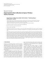
Desirableness Factor. We introduce the notion of desirable-
ness factor to measure the “suitableness” of a node to forward
packets.
Definition 1. Given a routing vector
−−→
S
1
S
0
,whereS
1
is
the source and S
0
is the sink, for forwarder F, the VBF
desirableness factor, α,ofanodeA,isdefinedasα

= p/W +
(R
−d ×cos θ)/R,wherep is the distance of A to the routing
vector
−−→
S
1
S
0
, d is the distance between node A and node F,
and θ is the angle between vector
−−→
FS
0
and vector
−→
FA. R is the
transmission range and W is the radius of the “routing pipe”
(i.e., the distance threshold).
EURASIP Journal on Wireless Communications and Networking 5
Source (S
1
)
Sink (S
0
)
W
W
R
F

p
d
A
(a)
Source (S
1
)
Sink (S
0
)
W
W
B
F
D
A
(b)
Figure 2: VBF illustration: (a) Desirableness Factor; (b) VBF with Self-Adaptation.
Figure 2(a) depicts the various parameters used in the
definition of desirableness factor. From the definition, we see
that for any node close enough to the routing vector, that is,
0
≤ p ≤ W, the desirableness factor of that this node is in the
range of [0, 3]. For a node, if its desirableness factor is large,
it means that either its distance to the routing vector is large
or it is not far away from the forwarder. In other words, it is
not desirable for this node to continue forwarding the packet.
On the other hand, if the desirableness factor of a node is 0,
then this node is on both the routing vector and the edge of
the transmission range of the forwarder. We call this node as

the optimal node, and its position as the best position.Forany
forwarder, there is at most one optimal node and one best
position. If the desirableness factor of a node is close to 0, it
means this node is close to the best position.
The Algorithm. We propose a self-adaptation algorithm
based on the concept of desirableness factor. This algorithm
aims to select the most desirable nodes as forwarders. In this
algorithm, when a node receives a packet, it first determines
if it is close enough to the routing vector. If yes, the node then
holds the packet for a time period related to its desirableness
factor. In other words, each qualified node delays forwarding
the packet by a time interval T
adaptation
, which is calculated as
follows:
T
adaptation
=
√
α
×T
delay
+
R
−d
v
0
,
(1)
where T

delay
is a predefined maximum delay, v
0
is the
propagation speed of acoustic signals in water, that is,
1500 m/s, and d is the distance between this node and the
forwarder. In the above equation, the first term reflects the
waiting time based on the node’s desirableness factor: the
more desirable (i.e., the smaller the desirableness factor), the
less time to wait. The second term represents the additional
time needed for all the nodes in the forwarder’s transmission
range to receive the acoustic signal from the forwarder.
During the delayed time period T
adaptation
,ifanode
receives duplicate packets from n other nodes, then this
node has to compute its desirableness factors relative to
these nodes, α
1
, , α
n
, and the original forwarder, α
0
.If
min(α
0
, α
1
, , α
n

) <α
c
/2
n
,whereα
c
is a predefined initial
value of desirableness factor (0
≤ α
c
≤ 3), then this node
forwards the packet; otherwise, it discards the packet.
Essentially, the above self-adaptation algorithm gives
higher priority to the desirable node to continue broadcast-
ing the packet, and it also allows a less desirable node to have
chances to reevaluate its “importance” in the neighborhood.
After receiving the same packets from its neighbors, the less
desirable node can measure its importance by computing
its desirableness factor relative to its neighbors. If there
are many more desirable nodes in the neighborhood, we
exponentially reduce the probability of this node to forward
the packet. That is, it is useless for this node to forward
the packet anymore since many other more desirable nodes
have forwarded the packet. In fact, if a node receives more
than two duplicate packets during its waiting time, it is most
likely that this node will not forward the packet no matter
what initial value α
c
takes. In this way, we can reduce the
computation overhead by skipping the reevaluation of the

desirableness factor.
From (1), we can see that the optimal node does not defer
forwarding packets in the self-adaptation algorithm. Thus,
we have the following lemma.
Lemma 2. If there exists an optimal path from the sender to the
target, that is, each node in the path is the optimal node for its
upstream node, then the self-adaptation algorithm selects this
path and entails no delay.
An Example. We illustrate VBF with self-adaptation in
Figure 2(b). In this figure, the forwarding path is specified
as the routing vector
−−→
S
1
S
0
from the source S
1
to the sink S
0
.
The node F is the current forwarder. There are three nodes,
namely, A, B,andD in its transmission range. Node A has the
smallest desirableness factor among these nodes. Therefore,
A has the shortest delay time and sends out the packet first.
As shown in this figure, node B is most likely to discard the
packet because it is in the transmission range of A and it has
to reevaluate the benefit to send the packet. Node D is out
of the transmission range of A; therefore, it also forwards the
packet.

6 EURASIP Journal on Wireless Communications and Networking
3.4. Summary of VBF. We have described the basic VBF
routing protocol and the self-adaptation algorithm. We can
see that VBF addresses the mobility of nodes in the network
effectively. The positioning of nodes is performed locally and
no global synchronization required. VBF has no requirement
for stable forward path. VBF is an energy efficient and
scalable protocol. (1) In VBF, no state information is required
for each node; therefore, it is scalable to the size of the
network. (2) In VBF, only the nodes close to the routing
vector are involved in packet forwarding, and all other nodes
are in idle state, thus saving energy. The self-adaptation
algorithm helps to further reduce energy consumption by
selecting more desirable nodes.
VBF is also robust and less computationally demanding.
(1) The success of data delivery is not dependent on the
stable neighborhood, but on the node density. If there exists
at least one path in the “routing pipe” specified by the
routing vector, then the packet can be successfully delivered.
(2) The computation demand on each node is appropriate
for routing on-demand since only simple vector-related
calculation is needed.
The routing pipe in VBF is determined by a predefined
radius. In sparse networks, if no nodes lie within this pipe,
then data packets cannot be forwarded to the sink even
though paths may exist outside the pipe. In basic VBF, these
paths will not be discovered and thus the delivery ratio will
be severely affected. To improve the performance of VBF in
sparse networks, we propose an enhanced version of VBF:
Hop-by-hop Vector-based Forwarding (HH-VBF).

3.5. VBF Enhancement: Hop-by-Hop Vector-Based Forwarding
(HH-VBF). In HH-VBF, we redefine the routing virtual pipe
to be a per-hop virtual pipe creation, instead of a unique
pipe from the source to the sink. This hop-by-hop approach
allows the expansion of the probability of finding a routing
path in comparison with VBF. Consider a node N
i
which
receives a packet from the source or a forwarder node S
j
.
Upon receipt of the packet, the node computes the vector
from the sender S
j
to the sink. In this way, the forwarding
pipe changes each hop in the network, giving the name hop-
by-hop vector-based forwarding (HH-VBF).Afterareceiver
computes the vector from its sender to the sink, it calculates
its distance to that vector. If this distance is smaller than the
predefined threshold, it is eligible to forward the packet. We
refer to such a node as a candidate forwarder for the packet.
As in VBF, each candidate forwarder maintains a self-
adaptation timer which depends on the desirableness factor.
The timer represents the time the node holds the packet
before forwarding it. We modify Definition 1 and get a new
definition of the desirableness factor for HH-VBF.
Definition 3. For a candidate forwarder F, the HH-VBF
desirableness factor, α

,ofanodeA,isdefinedas

α

=
(
R
−d × cos θ
)
R
,
(2)
where d is the distance between node A and node F,andθ
is the angle between
−−→
FS
0
and
−→
FA. R is the transmission range
and S
0
is the sink.
The self-adaption algorithm in HH-VBF is different from
that in the VBF. As we recall, due to the effective packet
suppression strategy adopted in VBF, only a few paths could
be selected to forward packets. This may cause problems
in sparse networks. To enhance the packet delivery ratio in
sparse networks, we introduce some redundancy control in
the self-adaption procedure for HH-VBF.
In HH-VBF, when a node receives a packet, it first holds
the packet for some time period proportional to its desirable-

ness factor (this is similar to VBF). Therefore, the node with
the smallest desirableness factor will send the packet first.
Following this way, each node in the neighborhood may hear
the same packet multiple times. HH-VBF allows each node
overhearing the duplicate packet transmissions to control the
forwarding of this packet as follows: the node calculates its
distances to the various vectors from the packet forwards to
the sink. If the minimum one of these distances is still larger
than a predefined minimum distance threshold β, this node
will forward the packet; otherwise, it simply drops the packet.
Obviously, the bigger β is, the more nodes will be allowed for
packet forwarding. Thus, HH-VBF can control forwarding
redundancy by adjusting β.
Each node that qualifies as a candidate forwarder delays
the packet forwarding by an interval T
adaptation
which is
computed the same way as in VBF. Then each node still uses
the self-adaptation algorithm to limit the redundant packets.
Compared with the basic VBF, HH-VBF has two signifi-
cant benefits: (1) more paths can be found for data delivery in
sparse networks; (2) HH-VBF is less sensitive to the routing
pipe radius (i.e., the distance threshold). Correspondingly,
we have the following two lemmas.
Lemma 4. Given the same routing pipe radius, if a packet is
routable in VBF, then it must be routable in HH-VBF.
Proof. If we can show that any routing-involved node in
VBF is also involved in routing in HH-VBF, then we prove
the lemma. Now, we assume that in HH-VBF, a node N
i

is
not involved in routing. This implies that in the network
no path leading from the source to N
i
gives the distance
threshold. Thus, the source-to-sink routing pipe of the basic
VBF protocol does not cover node N
i
; that is, N
i
is not
involved in routing. Using the contradiction method, we
prove the lemma.
Lemma 4 indicates that HH-VBF is at least as reliable as
VBF.
Lemma 5. The valid range of routing pipe radius of HH-VBF
is [0, R], while the valid range of VBF is [0, D],whereR is the
node transmission range, and D is the network diameter (here
one assumes that all nodes have the same transmission range).
Proof. In HH-VBF, each node makes packet forwarding
decisions based on its distance to the vector from its
forwarder to the sink. If the distance is smaller than the
predefined pipe radius, the node will forward the packet;
otherwise it will discard the packet. In this way, when the pipe
radius is bigger than the transmission range of the forwarder,
EURASIP Journal on Wireless Communications and Networking 7
those nodes which are outside the transmission range while
still lie in the routing pipe are useless since they can not
hear the packets from the forwarder. Thus, the valid range
of routing pipe radius of HH-VBF is [0,R], where R is the

transmission range.
In VBF, each node makes packet forwarding decisions
based on its distance to the vector from the source to the
sink. When the pipe radius is bigger than the transmission
range, those nodes which are outside the transmission range
of one forwarder while still lie in the routing pipe may hear
packets from other forwarder. This means that they may be
still eligible for packet forwarding. Thus, theoretically there is
no upper limit for the pipe radius of VBF, while in practice,
the valid range of routing pipe radius of VBF is [0, D], where
D is the network diameter.
In VBF, the bigger the pipe radius, the higher successful
data delivery ratio VBF can achieve, and the more optimal
the paths VBF can select. Thus, for networks with different
node densities, a proper pipe radius should be carefully
chosen. While for HH-VBF, from Lemma 5, we can see that
the biggest value of the pipe radius is R, which will clearly
yield the highest successful data delivery ratio. Thus, in HH-
VBF, we can eliminate the trouble of tuning the pipe radius
by simply choosing the transmission range R.
4. Performance Evaluation
In this section, we evaluate the performance of VBF and HH-
VBF through extensive simulations in NS-2.
4.1. Simulation Settings. In our simulations, sensor nodes are
randomly distributed in a 3D field of 1000 m
× 1000m ×
500 m. There are one data source and one sink. The source
is fixed at location (900, 900,500) near one corner of the
field at the floor, while the sink is at location (100, 100,0)
near the opposite corner at the surface. Besides the source

and the sink, all other nodes are mobile as follows: they can
move in horizontal two-dimensional space, that is, in the
X-Y plane (which is the most common mobility pattern in
underwater applications [36]). Each node randomly selects
a destination and moves toward that destination. Once the
node arrives at the destination, it randomly selects a new
destination and moves in a new direction. The sending rate
is set to be one packet per 10 seconds, which is low to reduce
interference among packets. For each simulation, the results
are averaged over 100 times, with a randomly generated
topology in each run. The total simulation time for each run
is 1000 seconds. We also implement a random access MAC
protocol for UWSNs in ns2. In this MAC protocol, when
a sender has packets to send, it first senses the channel. If
the channel is free, it sends out its packets. If the channel is
busy, it uses a back-off algorithm to contend the channel. The
maximum number of back-offsis4.
As to the parameter in the physical layer, we set the
parameters according to a commercial acoustic modem,
LinkQuest UWM1000 [38]: the bit rate is 10 kbps; the
transmission range is 100 meters; the energy consumptions
in sending mode, receiving mode and idle mode are 2 w,
0.75 w, and 8 mw, respectively. Further, we set the packet size
to 50 Bytes, the pipe radius to 100 meters for VBF, and the
predefined distance minimum threshold of HH-VBF, β to 75
meters.
Performance Metrics. We propose three metrics: success rate,
energy cost, and energy tax. Success rate is defined as the ratio
of the number of packets successfully received by the sink to
the number of packets generated by the source. Energy cost

is measured by the total energy consumption of all the nodes
in the network. Energy tax is defined as the average energy
consumption for each successfully received packet.
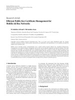
4.2. Impact of Density and Mobility. We first investigate
the impact of node density and mobility. In this set of
experiments, all the mobile nodes have the same speed. We
vary the mobility speed of each node from 0 m/s to 3 m/s
and the number of nodes from 500 to 4000. The simulation
results are plotted in Figures 3(a) and 3(b).
Figure 3(a) shows the success rate as the function of
the number of nodes and the speed of nodes. When the
node density is low, the success rate increases with density.
However, when more than 4000 nodes are deployed in the
space, the success rate remains above 90%. The success rate
decreases slightly when the nodes are mobile; however, it is
rather stable under different mobility speeds.
Figure 3(b) depicts the energy cost as the number of
nodes and the speed of nodes vary. The energy cost increases
when the number of nodes increases since more nodes are
involved in packet forwarding. For the same number of nodes
in the network, this figure also shows that the energy cost in
static networks is slightly less than that in dynamic networks.
However, the energy cost remains relatively stable as we vary
the mobility speed of nodes in the network.
This set of simulation experiments have shown that in
VBF, node speed has some impact on success rate and energy
cost, but not significantly. It demonstrates that VBF could
handle node mobility very effectively.
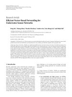
4.3. Impact of the Routing Pipe Radius. We test the impact
of the routing pipe radius (i.e., the distance threshold) in

this set of simulations. There are 2000 nodes in the network,
and their speed is fixed at 1.5 m/s. We vary the radius from 0
meters to 200 meters. The results are shown in Figures 4(b)
and 4(a).
From Figure 4(b), we can see that the success rate
increases as the radius is lifted; meanwhile, as shown
in Figure 4(a), more energy is consumed because more
qualified nodes forward the packets. The curve in Figure 4(b)
becomes flat when the radius exceeds 150 meters. This is
caused by the topology of the network and the positions of
the sink. The sink is located at the corner of a cube. It does
not help to improve the success rate further once the radius
exceeds some threshold since there are no nodes in routing
pipe near the sink.
As shown in the above figures, the routing pipe radius
does affect the given metrics greatly. In short, the bigger
8 EURASIP Journal on Wireless Communications and Networking
Success rate
0
0.2
0.4
0.6
0.8
1
Speed of nodes (m/s)
3
2
1
0
Number of nodes

1500
2000
2500
3000
3500
4000
(a) Impact of density and mobility on success rate
Energy consumption (Joul)
0
1
2
3
4
×10
4
Speed of nodes (m/s)
3
2
1
0
Number of nodes
1500
2000
2500
3000
3500
4000
(b) Impact of density and mobility on energy cost
Figure 3: The performance of VBF with varying density and mobility.
Energy consumption (joul)

1.6
1.8
2
2.2
2.4
2.6
2.8
3
×10
4
Radius
0 50 100 150 200
(a) Energy consumption versus routing pipe radius
Success rate
0
0.1
0.2
0.3
0.4
0.5
0.6
0.7
0.8
0.9
1
Radius
0 50 100 150 200
(b) Success rate versus routing pipe radius
Figure 4: The performance of VBF with varying routing pipe radius.
the radius is, the higher success rate VBF can achieve, the

more energy VBF consumes, and the more optimal path VBF
selects.
4.4. Effect of the Self-Adaptation Algorithm. In order to check
the effect of the self-adaptation algorithm, we implement two
versions of VBF, one is armed with self-adaptation algorithm,
and the other is not. We compare the performance of these
two implementations. In this set of simulation experiments,
the speed of each node is fixed at 1.5 m/s, and the routing
pipe radius is fixed at 100 m. The results are shown in Figures
5(a) and 5(b).
From Figure 5(a), we can see that even in a spare
network, VBF with self-adaptation algorithm spends only
half as much time as the one without self-adaptation algo-
rithm. When the number of nodes increases, the difference
between these two curves tends to increase, indicating that
the self-adaptation algorithm can save more energy when the
networks are densely deployed.
As shown in Figure 5(b), the success rate of VBF with
self-adaptation is slightly less than the one without self-
adaptation. However, the difference between these two
curves tends to dwindle as the number of nodes increases.
With more than 1000 nodes in the network, the difference
is less than 5%. This result shows that the side effect of the
self-adaptation algorithm diminishes in dense networks.
The results from this set of simulations show that the
self-adaptation algorithm can save energy effectively, espe-
cially for dense networks. Even though the self-adaptation
algorithm achieves this goal by introducing extra end-to-
end delay and slightly reducing success rate, the success rate
reduction is less than 10% in the sparse network case and

the extra end-to-end delay is also limited. Furthermore, these
side effects tend to disappear when the number of nodes
increases.
EURASIP Journal on Wireless Communications and Networking 9
Energy consumption
1
2
3
4
5
6
7
8
9
10
×10
4
Number of nodes
1500 2000 2500 3000 3500 4000
Self-adaption
Non-self-adaption
(a) Effects on energy consumption
Success rate
0
0.1
0.2
0.3
0.4
0.5
0.6

0.7
0.8
0.9
1
Number of nodes
1500 2000 2500 3000 3500 4000
Self-adaption
Non-self-adaption
(b) Effects on success rate
Figure 5: The performance of VBF with and without self-adaptation algorithm.
Success rate
0.7
0.75
0.8
0.85
0.9
0.95
1
Error probability
00.10.20.30.40.5
Packet-loss
Node-failure
Figure 6: The performance of VBF with varying packet loss and
node failure.
4.5. Robustness of VBF. In this set of simulations, we evaluate
the robustness of VBF against packet loss (or channel error)
and node failure. In the experiments, the number of nodes
is fixed at 1000, the radius is set 100 m, and the speed of
nodes is set 0 m/s. In order to increase the density of the
node deployment, we set the space to 500 m

×500m×500 m.
The source and the sink are located at (250.250,0) and
(250,250,500), respectively.
The simulation results are shown in Figure 6.Thex-axis
is the error probability, which has different meanings. For the
packet loss curve, node failure is set 0 and x-axis is packet
loss probability. For the node failure curve, packet loss is
fixed at 0 and the x-axisisnodefailureprobability.From
this figure, we can see that VBF is robust against both packet
loss and node failure. When the packet loss is as high as
50%, the success rate can still reach 90%. We also observe
that VBF is more robust against packet loss since the packet
in VBF is forwarded in interleaved forward paths. If a node
does not receive a packet from one forwarding node, this
node still has the chance to receive the same packet from
another forwarding node since the forwarding paths in VBF
are interleaved and redundant.
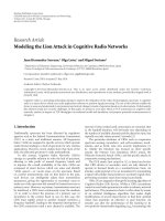
4.6. How HH-VBF Helps? In this simulation setting, we
compare the performance of VBF and HH-VBF in different
network scenarios and show that HH-VBF can greatly
improve the performance of VBF in sparse networks.
4.6.1. The Impact of Node Density. In this set of simulations,
we examine the impact of node density. We fix the node
speed at 0 (i.e., static networks) and change node density by
varying the number of nodes deployed in the field from 500
to 3000. The results for success rate, energy cost, and energy
tax are plotted in Figures 7(a), 7(b),and7(c),respectively.
From Figure 7(a), we can clearly observe the general
trend of success rate for both VBF and HHVBF: with the
increasing node density, the success rate is enhanced. This is

intuitive: for any node in the network, as the network density
becomes larger, more nodes will fall in its routing pipe (with
fixed radius as the transmission range). In other words, more
nodes are qualified for packet forwarding, as naturally leads
to higher success rate. Future, we can see that the success rate
of HH-VBF is significantly improved upon VBF, especially
when the network is sparse. This observation is consistent
with our early analysis: HH-VBF can find more paths for data
delivery in sparse networks.
10 EURASIP Journal on Wireless Communications and Networking
Success rate (%)
0
10
20
30
40
50
60
70
80
90
100
Number of nodes
500 1000 1500 2000 2500 3000
HH-VBF
VBF
(a) Success rate versus node density
Energy cost (J)
0
1

2
3
4
5
6
7
8
×10
4
Number of nodes
500 1000 1500 2000 2500 3000
HH-VBF
VBF
(b) Energy cost versus node density
Energy tax (J/pkt)
0
5
10
15
20
25
30
35
40
45
50
×10
2
Number of nodes
1000 1500 2000 2500 3000

HH-VBF
VBF
(c) Energy tax versus node density
Figure 7: The performance of HH-VBF with varying node density.
Figure 7(b) shows us that the energy cost of HH-VBF
is higher than that of VBF, and the gap becomes more
significant as the network gets denser. This is reasonable as
the higher the node density, the more paths HH-VBF can
find. We normalize the energy consumption, that is, compute
the energy tax, and the results are illustrated in Figure 7(c).
From this figure, we can observe that when the network is
sparse, the normalized energy cost of HH-VBF is greatly
lower than that of VBF. For example, when the number
of nodes is 1000, the energy tax of HH-VBF is 226 J/pkt,
while the energy overhead of VBF is as high as 4919 J/pkt.
This is mainly because the data delivery ratio of VBF is
extremely low (2% when the network size is 1000). This
further confirms that VBF is not good for sparse networks.
On the other hand, when the network gets denser, VBF shows
its advantage over HH-VBF: HH-VBF still tends to find more
paths, while the delivery ratio has reached the maximum. In
this case, more paths do not help to increase the success rate,
but more energy cost will be introduced.
4.6.2. The Impact of Node Mobility. In this set of simulations,
we explore how node mobility impacts the performance of
HH-VBF. We fix the network size at 1000 (a relatively sparse
network) and vary the node speed from 0 to 3 m/s. Figures
8(a), 8(b),and8(c) plot the results for the three metrics.
From Figure 8(a), we can observe that the node mobility has
different effects on the success rate of VBF and HH-VBF

when the node speed is low. By conducting many additional
EURASIP Journal on Wireless Communications and Networking 11
Success rate (%)
0
10
20
30
40
50
60
70
80
90
100
Speed of nodes (m/s)
00.511.522.53
HH-VBF
VBF
(a) Success rate versus node speed
Energy cost (J)
0
0.5
1
1.5
2
2.5
3
×10
4
Speed of nodes (m/s)

00.511.522.53
HH-VBF
VBF
(b) Energy cost versus node speed
Energy tax (J/pkt)
0
5
10
15
20
25
30
35
40
45
50
×10
2
Speed of nodes (m/s)
00.511.522.53
HH-VBF
VBF
(c) Energy tax versus node speed
Figure 8: The performance of HH-VBF with varying node speed.
simulation experiments, we find that this is mainly due to the
randomness of network topology generation. For VBF, when
node pattern changes from “static” to “mobile”, the mobility
actually helps to increase the chance that nonconnected paths
become connected, while for HH-VBF, since there are more
routing pipes in the network, light node mobility causes the

chance that nonconnected paths become connected smaller.
In fact, when the network is extremely sparse, for example,
the network size is 500 in our simulations, the impact of
light node mobility on HH-VBF has the same trend for
VBF: the success rate is slightly enhanced. In addition,
when we increase the number of simulation runs, the effect
of node mobility is decreased (due to space limit, these
results are not shown in in this paper). Furthermore, from
Figure 8(a), we can see that as the node speed gets higher,
the success rate of both VBF and HH-VBF becomes stable.
This indirectly confirms that experiencing more topologies
will help eliminate the difference caused by the topology
randomness.
Figures 8(b), 8(c),and8(a) together convey the major
information: both HH-VBF and VBF are robust to node
mobility, while HH-VBF has much better performance (in
terms of both success rate and energy tax) than VBF in sparse
networks.
To summarize, we evaluate the performance of VBF
under highly dynamic networks where almost all the nodes
are mobile. The results show that VBF addresses the node
mobility issue effectively and efficiently. In addition, these
results also show that self-adaptation algorithm contributes
significantly to save energy. Moreover, the simulation results
12 EURASIP Journal on Wireless Communications and Networking
show that VBF is robust against node failure and channel
error. Additionally, our simulation results also prove that
HH-VBF improves the success rate significantly and show
significant improvement in sparse networks.
5. Conclusions

In this paper, we have proposed a vector-based forwarding
(VBF) protocol to address the routing challenges in UWSNs.
VBF is scalable, robust, and energy efficient. (1) Packets
carry routing related information and no state information
is required at nodes. Thus, it is scalable in terms of network
size. (2) In VBF, only those nodes in the routing pipe
are involved in data forwarding. Therefore, it is energy
efficient. Moreover, our self-adaptation algorithm allows a
node to estimate its importance in its neighborhood and
thus adjust its forwarding policy to save more energy. (3)
VBF utilizes path redundancy (controlled by the routing
pipe radius) to provide robustness against packet loss and
node failure. To improve the performance of VBF in sparse
networks, we propose an enhanced version of VBF, hop-
by-hop vector-based forwarding (HH-VBF) protocol. HH-
VBF adopts multiple forwarding vectors in the networks
and, thus, improves the performance of VBF significantly in
sparse networks. Our simulation results have demonstrated
the promising performance of both VBF and HH-VBF.
Acknowledgments
This work is supported in part by the US National Science
Foundation under CAREER Grant no. 0644190, Grant
no. 0709005, Grant no. 0721834, Grant no. 0821597, and
the US Office of Navy Research under YIP Grant no.
N000140810864. Part of this work is presented in IFIP
Networking’06 [39].
References
[1] G. G. Xie and J. Gibson, “A networking protocol for underwa-
ter acoustic networks,” Tech. Rep. TR-CS-00-02, Department
of Computer Science, Naval Postgraduate School, Monterey,

Calif, USA, December 2000.
[2]J.G.Proakis,J.A.Rice,E.M.Sozer,andM.Stojanovic,
“Shallow water acoustic networks,” IEEE Communications
Magazine, vol. 39, no. 11, pp. 114–119, 2001.
[3]J.G.Proakis,E.M.Sozer,J.A.Rice,andM.Stojanovic,
“Shallow water acoustic networks,” IEEE Communications
Magazines, vol. 39, no. 11, pp. 114–119, 2001.
[4] I. F. Akyildiz, D. Pompili, and T. Melodia, “Challenges
for efficient communication in underwater acoustic sensor
networks,” ACM Sigbed Review, vol. 1, no. 1, pp. 3–8, 2004.
[5] J. Heidemann, W. Ye, J. Wills, A. Syed, and Y. Li, “Research
challenges and applications for underwater sensor network-
ing,” in Proceedongs of the IEEE Wireless Communications and
Networking Conference (WCNC ’06), vol. 1, pp. 228–235, Las
Vegas, Nev, USA, April 2006.
[6] J H. Cui, J. Kong, M. Gerla, and S. Zhou, “The challenges of
building scalable mobile underwater wireless sensor networks
for aquatic applications,” IEEE Network, vol. 20, no. 3, pp. 12–
18, 2006.
[7] J. Kong, J H. Cui, D. Wu, and M. Gerla, “Building underwater
adhoc networks for large scale real-time aquatic applications,”
in Proceedings of the IEEE Military Communication Conference
(MILCOM ’05), 2005.
[8] D. B. Kilfoyle and A. B. Baggeroer, “State of the art in
underwater acoustic telemetry,” IEEE Journal of Oceanic
Engineering, vol. 25, no. 1, pp. 4–27, 2000.
[9] P.Jacquet,P.M
¨
uhlethaler, T. Clausen, A. Laouiti, A. Qayyum,
and L. Viennot, “Optimized link state routing protocol for Ad

Hoc networks,” in Proceedings of the 5th IEEE International
Multi Topic Conference (INMIC ’01), 2001.
[10] R. Ogier, M. Lewis, and F. Templin, “Topology dissemination
based on reverse-path forwarding(TBRFP),” Tech. Rep. RFC
3684, IETF, Anaheim, Calif, USA, February 2004.
[11] C. Perkins and P. Bhagwat, “Highly dynamic destination-
sequenced distance-vector (DSDV) routing for mobile com-
puters,” in Proceedings of the ACM Conference on Communi-
cations Architectures, Protocols and Applications (SIGCOMM
’94), London, UK, August 1994.
[12] C. E. Perkins and E. Royer, “Ad-Hoc on-demand distance
vector routing,” in Proceedings of the IEEE Workshop on Mobile
Computing Systems and Applications (WMCSA ’99),New
Orleans, La, USA, February 1999.
[13] D. B. Johnson and D. A Maltz, “Dynamic source routing in
AdHocwirelessnetworks,”inMobile Computing, vol. 353
of Kluwer International Series in Engineering and Computer
Science, pp. 153–179, Kluwer Academic Publishers, Dodrecht,
The Netherlands, December 1996.
[14] C. Intanagonwiwat, R. Govindan, and D. Estrin, “Directed
diffusion: a scalable and roust communication paradigm for
sensor networks,” in Proceedings of the 6th Annual Inter-
national Conference on Mobile Computing and Networking
(MOBICOM ’00), Boston, Mass, USA, August 2000.
[15] F. Ye, H. Luo, J. Cheng, S. Lu, and L. Zhang, “A two-tier data
dissemination model for large-scale wireless sensor networks,”
in Proceedings of the 8th Annual International Conference on
Mobile Computing and Networking (MOBICOM ’02),Atlanta,
Ga, USA, September 2002.
[16] F. Ye, G. Zhong, S. Lu, and L. Zhang, “GRAdient broadcast: a

robust data delivery protocol for large scale sensor networks,”
ACM Wireless Networks, vol. 11, no. 3, pp. 285–298, 2005.
[17] M. Marina and S. Das, “On-demand multi path distance
vector routing in ad hoc networks,” in Proceedings of Interna-
tional Conference on Network Protocols (ICNP ’01), pp. 11–14,
Riverside, Calif, USA, November 2001.
[18] R. Leung, J. Liu, E. Poon, A. L. C. Chan, and B. Li, “MP-DSR:
a QoS-aware multi-path dynamic source routing protocol for
wireless ad-hoc networks,” in Proceedings of IEEE International
Conference on Local Computer Networks, Los Alamitos, Calif,
USA, 2001.
[19] D. Braginsky and D. Estrin, “Rumor routing algorithm
forsensornetworks,”inProceedings of the ACM Interna-
tional Workshop on Wireless Sensor Networks and Applications
(WSNA ’02), pp. 22–31, Atlanta, Ga, USA, September 2002.
[20] W. R. Heinzelman, J. Kulik, and H. Balakrishnan, “Adaptive
protocols for information dissemination in wireless sensor
networks,” in Proceedings of the 5th Annual ACM/IEEE
International Conference on Mobile Computing and Networking
(MOBICOM ’99), Seattle, Wash, USA, August 1999.
[21] B. Karp and H. T. Kung, “GPSR: greedy perimeter stateless
routing for wireless networks,” in Proceedings of the 6th Annual
International Conference on Mobile Computing and Networking
(MOBICOM ’00), pp. 243–254, Boston, Mass, USA, August
2000.
EURASIP Journal on Wireless Communications and Networking 13
[22] M. Heissenb
¨
uttel, T. Braun, T. Bernoulli, and M. W
¨

alchli,
“BLR: beacon-less routing algorithm for mobile ad hoc
networks,” Elsevier’s Computer Communication Journal, vol.
27, no. 11, pp. 1076–1086, 2003.
[23] H. F
¨
ußler, J. Widmer, M. K
¨
asemann, M. Mauve, and H.
Hartenstein, “Contention-based forwarding for mobile ad hoc
networks,” Elsevier’s Ad Hoc Networks, vol. 1, no. 4, pp. 351–
369, 2003.
[24] K. Seada, M. Zuniga, A. Helmy, and B. Krishnamachari,
“Energy-efficient forwarding strategies for geographic routing
in lossy wireless sensor networks,” in Proceedings of the
2nd International Conference on Embedded Networked Sensor
Systems (SenSys ’04), Baltimore, Md, USA, November 2004.
[25] S. Lee, B. Bhattacharjee, and S. Banerjee, “Efficient geographic
routing in multihop wireless networks,” in Proceedings of
the 6th ACM International Symposium on Mobile Ad Hoc
Networking and Computing (MobiHoc ’05), May 2005.
[26] D. Niculescu and B. Nath, “Trajectory based forwarding and
its applications,” in Proceedings of the 9th Annual International
Conference on Mobile Computing and Networking (MOBICOM
’03), San Diego, Calif, USA, September 2003.
[27] G. G. Xie and J. H. Gibson, “A network layer protocol for
UANs to address propagation delay induced performance lim-
itations,” in Prroceedings of the MTS/IEEE Oceans Conference,
pp. 1–8, Honolulu, Hawaii, USA, November 2001.
[28] D. Pompili and T. Melodia, “Three-dimenisional routing in

underwater acoustic sensor networks,” in Proceedings of the
2nd ACM Internat ional Workshop on Performance Evaluation
of Wireless Ad Hoc, Sensor, and Ubiquitous Networks (WASUN
’05), pp. 214–221, Montreal, Calif, USA, October 2005.
[29] A. Goel, A. G. Kannan, I. Katz, and R. Bartos, “Improving
efficiency of a flooding-based routing protocol for underwater
networks,” in Proceedings of the 3rd ACM International Work-
shop on Underwater Networks, pp. 91–94, San Francisco, Calif,
USA, September 2008.
[30]J.M.Jornet,M.Stojanovic,andM.Zorzi,“Focusedbeam
routing protocol for underwater acoustic networks,” in Pro-
ceedings of the 3rd ACM International Workshop on Underwater
Networks, pp. 75–81, San Francisco, Calif, USA, September
2008.
[31] Z. Guo, G. Colombi, B. Wang, J H. Cui, D. Maggiorinit, and
G. P. Rossi, “Adaptive routing in underwater delay/disruption
tolerant sensor networks,” in Proceedings of the 5th IEEE
Annual Conference on Wireless on Demand Network Systems
and Services (WONS ’08), pp. 31–39, Bavaria, Germany,
January 2008.
[32] T. C. Austin, R. P. Stokey, and K. M. Sharp, “PARADIGM:
a buoybased system for AUV navigation and tracking,” in
Proceedings of the MTS/IEEE Oceans Conference and Exhibition
(Oceans ’00), vol. 2, pp. 935–938, Providence, RI, USA, 2000.
[33] Y. Zhang and L. Cheng, “A distributed protocol for multi-
hop underwater robot positioning,” in Proceedings of the IEEE
International Conference on Robotics and Biomimetics, August
2004.
[34] J E. Garcia, “Ad hoc positioning for sensors in underwater
acoustic networks,” in Proceedings of the MTS/IEEE Oceans

Conference (Ocean ’04), vol. 4, pp. 2338–2340, 2004.
[35] N. H. Kussat, C. D. Chadwell, and R. Zimmerman, “Absolute
positioning of an autonomous underwater vehicle using
GPS and acoustic measurements,” IEEE Journal of Oceanic
Engineering, vol. 30, no. 1, pp. 153–164, 2005.
[36] Z. Zhou, J H. Cui, and S. Zhou, “Localization for large-
scale underwater sensor networks,” in Proceedings of the IFIP
International Conferences on Networking, pp. 108–119, Atlanta,
Ga, USA, May 2007.
[37] Z. Zhou, J H. Cui, and A. Bagtzoglou, “Scalable localization
with mobility prediction for underwater sensor networks,”
UCONN CSE Report UbiNet-TR07-01, July 2007.
[38] “LinkQuest,” />[39] P. Xie, J H. Cui, and L. Lao, “VBF: vector-based forwarding
protocol for underwater sensor networks,” in Proceedings of the
IFIP Working Conference on Networking, Coimbra, Portugal,
May 2006.