Báo cáo hóa học: " Research Article Joint Channel-Network Coding for the Gaussian Two-Way Two-Relay Network" docx

Hindawi Publishing Corporation
EURASIP Journal on Wireless Communications and Networking
Volume 2010, Article ID 708416, 13 pages
doi:10.1155/2010/708416

Research Article
Joint Channel-Network Coding for the Gaussian Two-Way
Two-Relay Network
Ping Hu,1 Chi Wan Sung,1 and Kenneth W. Shum2
1 Department
2 Department

of Electronic Engineering, City University of Hong Kong, Hong Kong
of Information Engineering, The Chinese University of Hong Kong, Hong Kong

Correspondence should be addressed to Kenneth W. Shum,
Received 1 October 2009; Revised 27 January 2010; Accepted 13 March 2010
Academic Editor: Sae-Young Chung
Copyright © 2010 Ping Hu et al. This is an open access article distributed under the Creative Commons Attribution License, which
permits unrestricted use, distribution, and reproduction in any medium, provided the original work is properly cited.
New aspects arise when generalizing two-way relay network with one relay to two-way relay network with multiple relays. To study
the essential features of the two-way multiple-relay network, we focus on the case of two relays in our work. The problem of
how two terminals, equipped with multiple antennas, exchange messages with the help of two relays is studied. Five transmission
strategies, namely, amplify-forward (AF), hybrid decode amplify forward (HLC), hybrid decode amplify forward (HMC), decode
forward (DF), and partial decode forward (PDF), are proposed. Their designs are based on a variety of techniques including
network coding, multiplexed coding, multi-input multi-output transmission, and multiple access with common information.
Their performance is compared with the cut-set outer bound. It is shown that there is no dominating strategy and the best strategy
depends on the channel conditions. However, by studying their multiplexing gains at high signal-tonoise (SNR) ratio, it is shown
that the AF scheme dominates the others in high SNR regime.

1. Introduction

Relay channel, which considers the communication between
a source node and a destination with the help of a relay
node, was introduced by van der Meulen in [1]. Based on
this channel model, Cover and El Gamal developed coding
strategies known as decode-forward (DF) and compressforward (CF) in [2]. These techniques now become standard
building blocks for cooperative and relaying networks, which
have been extensively studied in the literature (e.g., [3, 4]).
For many applications, communication is inherently
two-way. A typical example is the telephone service. In fact,
the study of two-way channel is not new and can be traced
back to Shannon’s work in 1961 [5]. However, the model
of two-way relay channel, though natural, did not attract
much attention. Recently, probably due to the advent of
network coding [6] in the last decade, there is a growing
interest in this model. The application of DF and CF to
two-way relay channel was considered in [7]. The halfduplex case was studied in [8, 9]. The results in [10] showed
that feedback is beneficial only in a two-way transmission.
Network coding for the two-way relay channel was studied

in [11, 12]. Physical layer network coding based on lattices is
considered recently [13], and shown to be within 0.5 bit from
the capacity in some special cases [14].
All the aforementioned works are for one relaying node.
It is easy to envisage that in real systems, more than one
relay can be used. Schein in [15] started the investigation
of the network with one source-destination pair and two
parallel relays in between. This model was further studied in
[16] under the assumption of half-duplex relay operations.
For one-way multiple-relay networks in general, cooperative
strategies were proposed and studied in [17]. We remark

that a notable feature that does not exist in the singlerelay case is that the multiple relays can act as a virtual
antenna array so that beamforming gain can be reaped at
the receiver. In this paper, we follow this line of research and
consider two-way communications. Two-relays are assumed,
for this simple model already captures the essential features
of the more general multiple-relay case. We are interested in
knowing how different techniques can be used to construct
transmission strategies for the two-way two-relay network
and how they perform under different channel conditions.
In particular, we apply the idea of network coding to both the


2

EURASIP Journal on Wireless Communications and Networking

physical layer and the network layer. Besides, channel coding
techniques for multiple access channel (MAC) and multiinput multi-output (MIMO) channel are also employed.
Several transmission strategies are thus constructed and their
achievable rate regions are derived.
We remark that the channel model that we consider
in this paper is also called the restricted two-way two-relay
channel [7]. This means that the signal from a source node
depends only on the message to be transmitted, but not
on the received signal at the source. Besides, our results are
obtained under the half-duplex assumption, which is realistic
for practical systems. Each node is assumed to transmit one
half of the time and receive during the other half of the time.
The performance of our proposed strategies can be further
improved if the ratio of transmission time and receiving time

is optimized. We do not consider this more general case, since
it complicates the analysis but provides no new insights.
This paper is organized as follows. Our network model
is described in Section 2. Some basic coding techniques are
reviewed in Section 3. Based on these coding techniques,
several transmission strategies are devised in Section 4. Their
performance at high signal-to-noise ratio regime is analyzed
in Section 5. The rate regions of these strategies are compared
under some typical channel realizations in Section 6. The
conclusion is drawn in Section 7.

1

hA1

hB1

A

B
hA2

hB2
2

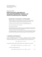
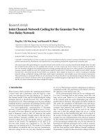
Figure 1: Model of two-way two-relay network. The labels of the
arrows indicate the corresponding link gains.

In the second stage, for t = N + 1, N + 2, . . . , 2N, the
outputs at the terminal nodes are

YA (t) = hA1 X1 (t) + hA2 X2 (t) + ZA (t),

(3)

YB (t) = hB2 X2 (t) + hB1 X1 (t) + ZB (t),

(4)

where X j (t) ∈ R, j ∈ {1, 2} is the transmit symbol of relay j,
Zi (t) ∈ Rn for i ∈ {A, B} is a Gaussian random vector with
each component i.i.d according to N (0, σ 2 ). We assume that
the link gains hA1 , hA2 , hB1 , and hB2 are time-invariant and
known to all nodes. We have the following power constraints
in each stage:
N

1
Xi (t)T Xi (t) ≤ Pi
N t=1

2. Channel Model and Notations
The two-way two-relay (TWTR) network consists of four
nodes: two terminals A and B, and two parallel relays 1
and 2 (see Figure 1). Terminals A and B want to exchange
messages with the help of the two relays. We assume there is
no direct link between the two terminals and between the
two-relays. Furthermore, all of the nodes are half-duplex.
The total communication time, 2N, are divided into two
stages, each of which consists of N time slots. In the first
stage, the terminals send signals and the relays receive. In the

second stage, the relays send signals and the terminals receive.
The solid arrows in Figure 1 correspond to stage 1 and the
dashed arrows correspond to stage 2.
Suppose that terminals A and B are equipped with n
antennas, whereas each of relays 1 and 2 has only one
antenna. For i ∈ {A, B} and j ∈ {1, 2}, we use Xi (t) ∈ Rn
to denote the transmit signal from node i, and Z j (t) ∈ R
to denote independently and identically distributed (i.i.d.)
Gaussian noise with distribution N (0, σ 2 ). The channel is
assumed static and the channel gain from node i to j is
denoted by an n-dimensional column vector hi j . We assume
channel reciprocity holds so that hi j = h ji . In the first stage,
the outputs of the network at time t = 1, 2, . . . , N, are given
by

(5)

for i ∈ {A, B}, and
2N

1
X 2 (t) ≤ P j
N t=N+1 j

(6)

for j ∈ {1, 2}, where PA , PB , P1 , and P2 denote the
power constraints on terminals A and B and relays 1 and 2,
respectively.
Let RA and RB be the data rates of terminal A and B,

respectively. In a period consisting of 2N channel symbols (N
symbols for each phase), terminal A wants to send one of the
22NRA symbols to terminal B, and terminal B wants to send
one of the 22NRB symbols to terminal A. A (22NRA , 22NRB , 2N)
code for the TWTR network consists of two message sets
MA = {1, 2, . . . , 22NRA } and MB = {1, 2, . . . , 22NRB }, two
encoding functions
fi : Mi −→ (Rn )N ,

i ∈ {A, B},

(7)

j ∈ {1, 2},

(8)

two relay functions
φ j : RN −→ RN ,
and two decoding functions
gA : (Rn )N × MA −→ MB ,
(9)

Y1 (t) = hT XA (t) + hT XB (t) + Z1 (t),
A1
B1

(1)

gB : (Rn )N × MB −→ MA .

Y2 (t) = hT XA (t) + hT XB (t) + Z2 (t).
A2
B2

(2)

For i = A, B, terminal i transmits the codeword fi (mi ) in
stage one, where mi is the message to be transmitted. For


EURASIP Journal on Wireless Communications and Networking
j = 1, 2, relay j applies the function φ j to its received
signal and transmits the resulting signal in the second stage.
Let the received signals at terminals A and B be YN and
A
YN , respectively. In this paper, we will use a superscript
B
“YN ” to indicate a sequence of length N. So YN and YN
A
B
are sequences of length N, with each component equal to
a vector in Rn . After the second stage, terminal i decodes
the message from the other source node by gi . We note
that the decoding function gi uses the message from source
terminal i as input as well. We say that a decoding error
occurs if gA (YN , mA ) = mB or gB (YN , mB ) = mA . The average
/
/
A

B
probability of error is
2N
Pe

3

C(x)
0.25log2 (1 + x). Also, for n × n matrices, we let
Cn (X)
0.25log2 det(In + X), where In denote the n × n
identity matrix. The reason for the factor of 0.25 before the
log function, instead of a factor of 0.5 in the original capacity
formula, is due to the fact that the total transmission time is
divided into two stages of equal length. All logarithms in this
paper are in base 2. The set of non-negative real numbers is
denoted by R+ . Gaussian distribution with mean zero and
covariance matrix K is denoted by N (0, K).

3. Review of Coding Techniques and Capacity
Regions from Information Theory

1
The proposed transmission strategies are based on a host of
existing coding techniques and capacity results. A review of
them is given in this section.

|MA ||MB |

Pr gA YN , mA = mB , or

/
A

×
(mA ,mB )
∈MA ×MB

gB YN , mB
B

= mA | (mA , mB ) is sent .
/

(10)
A rate pair (RA , RB ) is said to be achievable if there exists
a sequence of (22NRA , 22NRB , 2N) codes, satisfying the power
2N
constraints in (5) and (6), with Pe → 0 as N → ∞.
Although the terminals are equipped with n antennas,
the transmitted signals from the terminals are essentially 2
dimensional. To see this, we observe that the first term in
the right hand side of (1), namely, hT XA (t), is a projection
A1
of XA (t) in the direction of hA1 . Any signal component of
XA (t) orthogonal to hA1 will not be picked up by relay 1.
Likewise, from (2), we see that any signal component of
XA (t) orthogonal to hA2 will not be sensed by relay 2. There is
no loss of generality, if we assume that the signals transmitted
from the terminals take the following form:
Xi (t) = Hi λi (t)

(11)

for i ∈ {A, B}, where Hi
[hi1 hi2 ] is an n × 2 matrix,
and the two components in λi (t) [λi1 (t) λi2 (t)]T represent
the projections of Xi (t) on hi1 and hi2 . We consider the 2dimensional vector λi (t) as the input to the channel at node
i. The power constraint in (5) can be written as
N

1
λi (t)T HT Hi λi (t) ≤ Pi ,
i
N t=1

(12)

for i ∈ {A, B}.
Notations. We will treat 2 × 1 random vectors λA and λB as
input signals at terminal A and B, respectively, and let KA and
KB denote their corresponding 2 × 2 covariance matrices. For
i ∈ {A, B} and j ∈ {1, 2}, let
Γij

hTj Hi Ki HT hi j
i
i
σ2

(13)

be the signal to noise ratio of the signal received at relay j
from terminal i. Shannon’s capacity formula is denoted by

3.1. Physical-Layer Network Coding. In wireless channel, the
channel is inherently additive; the received signal is a linear
combination of the transmitted signals. This fact is exploited
for the two-way relay channel in [18–21]. Consider the
following single-antenna two-way network with two sources
and one relay in between. There is no direct link between the
two sources, and the exchange of data is done via the relay
node in the middle. Let xi (t) be the transmitted signal from
source i, for i = 1, 2. The transmission is divided into two
phases. In the first phase, the relay receives
y(t) = x1 (t) + x2 (t) + z(t),

(14)

where z(t) is an additive noise. For simplicity, it is assumed
that both link gains from the sources to the relay are equal
to one. In the second phase, the relay amplifies the received
signal y(t), and transmits a scaled version ζ y(t) of y(t),
where ζ is a scalar chosen so that the power requirement
is met. Since source 1 knows x1 (t), the component ζx1 (t)
within the received signal at source 1 can be treated as known
interference, and hence be subtracted. Similarly, source 2 can
subtract ζx2 (t) from the received signal. Decoding is then
based on the signal after interference subtraction.
3.2. Multiplexed Coding. Multiplexed coding [22] is a useful
coding technique for multi-user scenarios in which some

user knows the message of another user a priori. Consider
the two-way relay channel as in the previous paragraph.
Node 1 wants to send message m1 to node 2 via the relay
node, and node 2 wants to send message m2 to node 1
via the relay node. For i = 1, 2, let ni be the number of
bits used to represent message mi . The transmission of the
nodes is divided into two phases. In the first phase, the two
source nodes transmit. Suppose that the relay node is able to
decode m1 and m2 . For the encoder at the relay, we generate a
2n1 × 2n2 array of codewords. Each codeword is independently
drawn according to the Gaussian distribution such that the
total power of each codeword is less than or equal to P. In
the second phase, the relay node sends the codeword in the
(m1 , m2 )-entry in this array. Suppose that the received signal
at source node i is corrupted by additive white Gaussian


4

EURASIP Journal on Wireless Communications and Networking

noise with variance σi2 , for i = 1, 2. At source 1, since m1
is known, the decoder knows that one of the 2n2 codewords
in the row corresponding to m1 had been transmitted. Out
of these 2n2 codewords, it then declares the one based on the
maximal likelihood criterion. By the channel coding theorem
for the point-to-point Gaussian channel, source 1 can decode
2
reliably at a rate of 0.5 log(1 + P/σ1 ). Likewise, by considering
the columns in the array of codewords, source 2 can decode

2
at a rate of 0.5 log(1 + P/σ2 ).
Multiplexed coding can be implemented using concepts
from network coding. We assume, without loss of generality,
that n2 ≥ n1 . We identify the 2n2 possible messages from
source node 2 with the vectors in the n2 -dimensional vector
space over the finite field of size 2, Fn2 , and identify the
2
2n1 messages from source node 1 with a subspace of Fn2 of
2
dimension n1 , say V1 . We generate 2n2 Gaussian codewords
independently, one for each vector in Fn2 . To send messages
2
m1 and m2 in the second phase, the relay node transmits
the codeword corresponding to m1 + m2 , where the addition
is performed using arithmetics in Fn2 . The output of the
2
decoder at node 1 is a vector in Fn2 . We subtract from it the
2
vector in V1 corresponding to m1 . If there is no decoding
error, this gives the codeword corresponding to m2 , and the
value of m2 is recovered.
Now let us consider node 2. Since m2 is known a priori,
node 2 is certain that the signal transmitted from the relay
is associated with one of the vectors in the affine space
m2 + V1 . The message m1 can be estimated by comparing
the likelihood function of the 2n1 codewords associated with
m2 + V1 . It can be seen that the maximal data rate is the
same as in the array approach mentioned in the previous
paragraph, but the size of the codebook at the relay reduces

from 2n2 +n1 to 2n2 .
3.3. Capacity Region for MIMO Channel. Consider a MIMO
channel with nT transmit antennas and nR receive antennas,
with the link gain matrix denoted by a real nR × nT matrix H.
The channel output equals
Y = HX + Z,

(15)

where X is the nT -dimensional channel input and Z is an
nR -dimensional zero-mean colored Gaussian noise vector
with covariance matrix KZ . Without loss of information, we
whiten the noise by pre-multiplying both sides of (15) by
−
KZ 1/2 . The transformed channel output is thus
−
−
Y = KZ 1/2 HX + KZ 1/2 Z.

(16)

−
The covariance matrix of the noise vector KZ 1/2 Z is now the
nR × nR identity matrix. By the capacity formula for MIMO
channel with white Gaussian noise [23], the capacity for the
MIMO channel in (15) is given by

1
−
−

log det InR + KZ 1/2 HKX HT KZ 1/2 ,
2

(17)

where KX denotes the nR × nR covariance matrix of X. Using
the identity
det(In + AB) ≡ det(Im + BA),

(18)

which holds for any n × m matrix A and m × n matrix B, we
rewrite (17) as
1
−
log det InT + HT KZ 1 HKX .
2

(19)

3.4. Capacity Region for Multiple-Access Channel (MAC).
The channel output of the two-user single-antenna Gaussian
multiple-access channel is given by
y = x1 + x2 + z,

(20)

where xi is the signal from user i, for i = 1, 2, and z is an
additive white Gaussian noise with variance σ 2 . Each of the
two users wants to send some bits to the common receiver.

Suppose that the power of user i is limited to Pi , for i = 1, 2.
The rate pair (R1 , R2 ), where Ri is the data rate of user i, is
achievable in the above 2-user MAC if and only if it belongs
to
Cmac

P1 P2
,
σ2 σ2

(R1 , R2 ) ∈ R2 :
+

(21)

R1 ≤ 0.5log2 1 +

P1
σ2

(22)

R2 ≤ 0.5log2 1 +

P2
σ2

(23)

R1 + R2 ≤ 0.5log2 1 +

(P1 + P2 )
σ2

.
(24)

We refer the reader to [24] for more details on the optimal
coding scheme for MAC.

4. Channel-Network Coding Strategies
We develop five transmission schemes for TWTR network.
In the first scheme (AF), the received signals at both relay
nodes are amplified and forwarded back to terminals A and
B. In the second and third scheme (HLC, HMC), one of
the relays employs the amplify forward strategy, while the
other decodes the messages from terminals A and B. In
the fourth scheme (DF), both relays decode the messages
from terminals A and B. In the last strategy (PDF), another
mixture of decode-forward and amplify-forward strategy is
described.
4.1. Amplify Forward (AF). In this strategy, relay node j
( j ∈ {1, 2}) buffers the signal received in the first stage, and
amplifies it by a factor of ζ j . The amplified signal
X j (t) = ζ j hT j XA (t) + hT j XB (t) + Z j (t)
A
B

(25)

is then transmitted in the second stage. At the end of the
second stage, each terminal, who has the information of
itself, subtracts the corresponding term and obtains the
desired message from the residual signal.


EURASIP Journal on Wireless Communications and Networking
By putting (25) into (3), we can write the received signal
at terminal A as
YA (t) = ζ1 hA1 hT + ζ2 hA2 hT HA λA (t)
A1
A2
+ ζ1 hA1 hT + ζ2 hA2 hT HB λB (t)
B1
B2

(26)

+ ζ1 hA1 Z1 (t) + ζ2 hA2 Z2 (t) + ZA (t).
Here, we have replaced XA (t) and XB (t) by their 2dimensional representations HA λA (t) and HB λB (t). Since
terminal A knows its own input λA (t) as well as the link gains
and amplifying factors, the signal component containing
λA (t) as a factor can be subtracted from YA (t). The residual
signal is
ζ1 hA1 hT + ζ2 hA2 hT HB λB (t)
B1
B2

(27)

+ ζ1 hA1 Z1 (t) + ζ2 hA2 Z2 (t) + ZA (t).
The message from terminal B can then be decoded using a
decoding algorithm for point-to-point MIMO channel. The
received signal at terminal B is treated similarly.
Theorem 1. A rate pair (RA , RB ) is achievable by the AF
strategy if
RA ≤ C2 HT HT NB
A af
af
RB ≤

C2 HT Haf
B

NA
af

−1

−1

Haf HA KA ,
(28)
HT HB KB
af

,

5

from terminals A and B, and meanwhile, relay 2 employs the
amplify-forward strategy. In order to obtain beamforming
gain, after decoding the two messages, relay 1 reconstructs
the codewords corresponding to the decoded messages and
sends a linear combination of them in the second stage.
In the first stage, relay 1 and terminals A and B form a
multiple-access channel with relay 1 as the destination node.
We use the optimal encoding scheme for MAC at terminals
A and B, and the optimal decoding scheme at relay 1. In
the second stage, relay 1 decodes and reconstructs XA (t) and
XB (t), and then transmits a linear combination
X1 (t) = zT XA (t) + zT XB (t)
A
B

for some zA and zB ∈ Rn . Relay 2 amplifies Y2 (t) by a scalar
factor ζ and transmits X2 (t) = ζY2 (t).
At terminal A, after subtracting the signal component
that involves XA (t), we get
hA1 zT + ζhA2 hT HB λB (t) + ζhA2 Z2 (t) + ZA (t).
B
B2

hB1 zT + ζhB2 hT HA λA (t) + ζhB2 Z2 (t) + ZB (t).
A
A2

Haf

ζ1 hB1 hT

A1

Theorem 2. A rate pair (RA , RB ) is achievable by the HLC
strategy if

i ∈ {A, B},

RA ≤ C2

+ ζ2 hB2 hT ,
A2

HA
hlc

RB ≤ C2

(29)

ζ1 , ζ2 ∈ R and KA and KB are 2 × 2 covariance matrices, such
that the following power constraints:

(34)

The decoding is done by using decoding method for MIMO
channel.

1
(RA , RB ) ∈ Cmac ΓA , ΓB ,
1

1
2
2
2
ζ1 hi1 hT + ζ2 hi2 hT + In σ 2 ,
i1
i2

(33)

At terminal B, the residual signal after subtraction is

where
Niaf

(32)

HB
hlc

T

T

NB
hlc
NA
hlc

−1

HA KA ,
hlc

−1

HB KB ,
hlc

(35)
(36)
(37)

where

Tr Hi Ki HT ≤ Pi ,
i

for i = A, B,

(30)

HA
hlc

hB1 zT + ζhB2 hT HA ,
A
A2

ΓA + ΓB + 1 ζ 2 σ 2 ≤ P j ,

j
j
j

for j = 1, 2,

(31)

HB
hlc

hA1 zT + ζhA2 hT HB ,
B
B2

are satisfied.

Nihlc

ζ 2 hi2 hT + In σ 2 ,
i2

(38)

for i = A, B,

Proof. The residual signal (27) at terminal A can be written
as HT HB λB (t) plus a noise vector with covariance matrix
af
NA . The residual signal at terminal B equals Haf HA λA (t)

af
plus a noise vector with covariance matrix NB . Therefore,
af
after self-signal subtraction, the resultant channels can be
considered MIMO channels with two transmit antennas and
n receive antennas. From (19), we obtain the rate constraints
in (28). The inequalities in (30) are the power constraints
for terminals A and B, and those in (31) are the power
constraints for relays 1 and 2.

zA , zB ∈ Rn , ζ ∈ R, and KA and KB are 2 × 2 covariance
matrices such that the following power constraints:

4.2. Hybrid Decode-Amplify Forward with Linear Combination (HLC). In this strategy, relay 1 decodes the messages

In (35), the product of a real number x and a set A is
defined as xA {xa : a ∈ A}.

Tr Hi Ki HT ≤ Pi ,
i

for i = A, B,

zT HA KA HT zA + zT HB KB HT zB ≤ P1 ,
A
A
B
B
ΓA + ΓB + 1 ζ 2 σ 2 ≤ P2
2

2

(39)
(40)
(41)

are satisfied.


6

EURASIP Journal on Wireless Communications and Networking

Proof. From the rate constraints for MAC channel in (22)–
(24), we have the rate constraints for relay 1 in (35). We
multiply by a factor of one half because the first phase only
occupies half of the total transmission time.
The conditions in (36) and (37) are derived from the
capacity formula for MIMO channel with colored noise in
(19). The inequalities in (39) are the power constraints for
sources A and B. The inequalities in (40) and (41) are the
power constraints for relays 1 and 2, respectively.
The parameters zA , zB , KA , and KB can be obtained by
running an optimization algorithm. For example, we can aim
at maximizing a weighted sum wA RA + wB RB . The values of
zA , zB , KA and KB which maximize the weighted sum wA RA +
wB RB are chosen.
4.3. Hybrid Decode-Amplify Forward with Multiplexed Coding
(HMC). As in the previous strategy, relay 1 decodes and
forwards the messages from A and B, and relay 2 amplifies

and transmits the received signal. However, in this strategy,
relay 1 re-encodes the messages into a new codeword to be
sent out in the second stage. Terminals A and B decode the
desired messages based on multiplexed coding.
Theorem 3. A rate pair (RA , RB ) is achievable by the HMC
strategy if RA and RB satisfy
(RA , RB ) ∈

1
Cmac ΓA , ΓB ,
1
1
2

RA ≤ Cn GA NB
hmc
hmc
RB ≤ Cn GB NA
hmc
hmc

−1

−1

(42)

,

(43)

,

(44)

where
GA
hmc

hB1 hT P1 + ζ 2 hB2 hT HA KA HT hA2 hT ,
B1
A2
A
B2

(45)

GB
hmc

hA1 hT P1 + ζ 2 hA2 hT HB KB HT hB2 hT ,
A1
B2
B
A2

(46)

Nihmc

ζ 2 hi2 hT + In σ 2 ,
i2

for i ∈ {A, B},

(47)

KA , KB are 2 × 2 covariance matrices satisfying (39), and ζ ∈ R
satisfies (41).
Proof. The proof is by random coding argument and we will
sketch the proof below. More details can be found in [25].
Our objective is to show that any rate pair (RA , RB ) that
satisfies the condition in the theorem is achievable. For i =
A, B, terminal i randomly generates a Gaussian codebook
with 22NRi codewords with length N, satisfying the power
constraint in (5). Label the codewords by XiN (mi ), for mi ∈
Mi . For relay 1, we generate a 22NRA × 22NRB array of Gaussian
codewords of length N and power P1 . The codeword in row
N
mA and column mB is denoted by X1 (mA , mB ), and satisfies
the power constraint in (6).
After the first stage, relay 1 is required to decode both
messages from terminals A and B. This can be accomplished with arbitrarily small probability of error if the

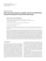
mAc , mBc , mAp
1

A

B

2
mAc , mBc , mB p

Figure 2: Decoded messages at the two-relays in the DF strategy.

rate constraints for MAC in (22) to (24) are satisfied. This
corresponds to the rate constraint in (42). Let the estimated
messages from A and B be mA and mB .
N
In the second stage, relay 1 transmits X1 (mA , mB ). Relay
2 amplifies its received signal and transmits ζY2 (t). From
(41), the amplified signal has average power no more than
P2 .
After subtracting the term ζhA2 hT XA (t), which is known
A2
to terminal A, the residual signal at terminal A is
hA1 X1 (mA , mB )(t) + ζhA2 hT XB (t) + ζhA2 Z2 (t) + ZA (t).
B2
(48)
Note that terminal A knows its message mA , and mA = mA
with probability arbitrarily close to one if (42) is satisfied.
The idea of multiplexed coding can then be used. In (48), the
covariance matrix of the signal in square bracket is given by
GB in (46), and the covariance of the noise term is given by
hmc
NA . Applying the capacity expression, we obtain the rate
hmc
constraint in (44). In a similar manner, we obtain (43).
4.4. Decode Forward (DF). In the DF strategy, terminal

node i, (i ∈ {A, B}) splits the message mi into two parts:
the common part mic and the private part mip . The two
common messages are transmitted via both relay nodes. The
private message mAp is decoded by relay 1 only, and can
be interpreted as going through the path from terminal A
to relay 1 to terminal B. Symmetrically, the private part
of message mB p is decoded by relay 2 only, and can be
interpreted as going through the path from terminal B to
relay 2 to terminal A. After the first stage, relay 1 decodes the
common messages of both terminals and the private message
of terminal A. Relay 2 decodes the common messages of
both terminals and the private message of terminal B. The
encoding and decoding schemes in the first stage is similar to
those developed by Han and Kobayashi for the interference
channel (IC) in [26]. Since both relays have access to the
common messages, the channel in the second stage can
be considered a multiple access channel with common
information. Furthermore, since terminals A and B have
information of themselves, we can further improve the rate
region by the idea of multiplexed coding.


EURASIP Journal on Wireless Communications and Networking
We have the following characterization of the rate region
for the DF strategy:

Theorem 5. A rate pair (RA , RB ) is achievable by the PDF
strategy if it satisfies
⎧ ⎛
⎞ ⎛

⎞⎫
⎨
ΓA ⎠ ⎝ ΓA ⎠⎬
1
2
,C
,
RA ≤ min⎩C ⎝ B
Γ1 + 1
ΓB + 1 ⎭
2

Theorem 4. For i ∈ {A, B}, let Rip and Ric be the rates of the
private and common messages, respectively, from terminal i. Let
Γ j denote P j /σ 2 for j = 1, 2, and let KAc , KAp , KBc , and KB p
denote 2 × 2 covariance matrices, and
hTj Hi Kik HT hi j
i
i
σ2

Γik
j

RA ≤ C2 (HB )T NB
pdf

(49)

for i ∈ {A, B}, j ∈ {1, 2} and k ∈ { p, c}. For j = 1, 2. A rate

pair (RA , RB ) is achievable if we can decompose RA = RAp +RAc
and RB = RB p + RBc such that

7

RB ≤ C2

HB
pdf

T

NA
pdf

−1

HB KR ,

−1

HB KB ,
pdf

(58)
(59)
(60)

where
Nipdf

2
2
ζ1 hi1 hT + ζ2 hi2 hT + In σ 2 ,
i1
i2

HB
pdf

ζ1 hA1 hT + ζ2 hA2 hT HB ,
B1
B2

(61)
1
(RA , RBc ) ∈ Cmac
2

Ap
Γ1 + ΓAc
1
,
Bp
Γ1 + 1

1
ΓAc
(RAc , RB ) ∈ Cmac Ac2 ,
2

Γ2 + 1

ΓBc
1
Bp
Γ1 + 1

Bp
Γ2 + ΓBc
2
ΓAc + 1
2

,

(50)

,

(51)

RAp ≤ C α1 hB1 2 Γ1 ,

and ζ j ∈ R and KA , KB , KR are 2 × 2 covariance matrices such
that the following power constraints hold
Tr Hi Ki HT ≤ Pi ,
i

for i = A, B,

(62)

(52)

KR j, j + ΓB + 1 σ 2 ζ 2 ≤ P j
j
j

(53)

for j = 1, 2. (Here, KR ( j, j) denotes the jth diagonal entry in
KR .)

RA ≤ Cn Γ1 hB1 hT + Γ2 hB2 hT
B1
B2
+ α1 α2 Γ1 Γ2 hB1 hT + hB2 hT
B2
B1

,

2

RB p ≤ C α2 hA2 Γ2 ,

(54)

RB ≤ Cn Γ1 hA1 hT + Γ2 hA2 hT
A1

A2
(55)
+ α1 α2 Γ1 Γ2 hA1 hT + hA2 hT
A2
A1
Tr HA KAc + KAp HT < PA ,
A

,
(56)

Tr HB KBc + KB p HT < PB ,
B
(57)
α1 + α1 < 1,

α2 + α2 < 1

for some nonnegative α j and α j .
Details of the DF coding scheme and the proof of
Theorem 4 are given in the Appendix.
4.5. Partial Decode Forward (PDF). In the PDF strategy,
both relays decode the message of terminal A. Each relay
then subtracts the reconstructed signal of terminal A from
the received signal. Call the resulting signal the residual
signal. The message of terminal A is re-encoded into a new
codeword, and linearly combined with the residual signal.
This linear combination is then transmitted in the second
stage. Since both relays know the message of terminal A, the
two-relays can jointly re-encode the message of terminal A

using some encoding scheme for a MIMO channel with two
transmit antennas and n receive antennas.

(63)

Proof. The two-relays treat the signal originated from terminal B as noise, and decode the message of terminal A.
The rate requirement in (58) guarantees that the message of
terminal A can be decoded with arbitrarily small probability
of error at both relays. Let the decoded message of terminal
A be denoted by mA .
For j = 1, 2, the reconstructed signal hT j XA (t) is then
A
subtracted from Y j (t). The residual signal at relay j is
hT j XB (t) + Z j (t).
B
At the relays, we employ two Gaussian codebooks for
the re-encoding of the message from terminal A. For each
message mA , we generate two correlated codewords U1,mA (t)
and U2,mA (t), with mean zero and each pair of symbols at any
t distributed according to a 2 × 2 covariance matrix KR . At
relay j, the decoded message mA is re-encoded into U j,mA (t),
which is a codeword with power KR ( j, j). In the second stage,
relay j transmits
U j,mA (t) + ζ j hT j XB (t) + Z j (t) ,
B

(64)

for some amplifying factor ζ j . The inequality in (63) ensures
that the power constraint is satisfied at the relays.

At the end of stage 2, terminal A subtracts the signal
component that involves U1,mA and U2,mA from its received
signal and obtains
HB λB (t) + ζ1 hA1 Z1 (t) + ζ2 hA2 Z2 (t) + ZA (t).
pdf

(65)

From the capacity formula for MIMO channel (19), terminal
A can recover the message from terminal B reliably if (60) is
satisfied.


8

EURASIP Journal on Wireless Communications and Networking

For the decoding in terminal B, we subtract all terms
involving XB (t), and get
HB

U1,mA (t)
+ ζ1 hB1 Z1 (t) + ζ2 hB2 Z2 (t) + ZB (t).
U2,mA (t)

(66)

This is equivalent to a MIMO channel with link gain matrix
HB and colored noise. Recall that KR is the covariance matrix
of the encoded signal. By the capacity formula of MIMO

channel (19), we obtain the rate constraint in (59).
Remark 1. We note that the matrices Niaf , Nihlc , Nihmc and
Nipdf , for i = A, B, are invertible. Indeed, by checking that
vT Nv is strictly positive for all non-zero v ∈ Rn , we see that
the matrix is positive definite, and hence invertible.

5. Performance in High SNR Regime
In this section, we compare the performance of the five
strategies described in the previous section in the high
Signal-to-Noise Ratio (SNR) regime.
For fixed powers and link gains, let Csum (σ 2 ) denote the
sum rate RA + RB as a function of the noise variance σ 2 . We
use the multiplexing gain (also called degree of freedom) [27],
defined by
M

Csum σ 2
,
→ 0 (1/2) log(σ −2 )

lim
2

σ

(67)

as the performance measure at high SNR. At high SNR, that
is, when σ 2 is very small, we can approximate the sum rate by
(M/2) log(σ −2 ) if the multiplexing gain is equal to M.

Consider the multiplexing gain of the AF scheme. When
the sum rate RA + RB is maximized subject to the rate
constraints (28) in Theorem 1, the equalities in (28) hold.
We can assume without loss of generality that
RA = C2 HT HT NB
A af
af
RB = C2 HT Haf NA
B
af

−1

−1

Haf HA KA ,

(68)

HT HB KB .
af

(69)

We first suppose that the covariance matrices KA and KB ,
and the amplifying constants ζ1 and ζ2 , are fixed. Note that if
the power constraint in (31) holds, then it continues to hold
if σ 2 becomes smaller. Therefore, when σ 2 → 0, the power
constraints in (30) and (31) are satisfied.
Each of the expressions in (68) and (69) can be written in

the form
M
1
log det I2 + 2 ,
4
σ

(70)

where M is a 2 × 2 matrix that equals
HT HT NB
A af
af

−1

HT Haf NA
B
af

Haf HA KA ,
−1

HT HB KB .
af

and Λ = [λi j ] is a diagonal matrix with non-negative
diagonal entries λ11 ≥ λ22 ≥ 0. The number of positive
diagonal entries in Λ is precisely the rank of M. We can
rewrite (70) as

Λ
1
log det U−1 V−1 + 2 .
4
σ

Suppose that U−1 V−1 is equal to [ai j ]2 j =1 . The determinant
i,

a21

By singular value decomposition [28, Chapter 7], we can
factor M as UΛV, where U and V are 2 × 2 unitary matrices,

a12
λ
a22 + 22
σ2

(74)

in (73) can be expanded as a polynomial in σ −2 , with the
degree equal to the rank of M. Therefore, the limit
(1/4) log det I2 + M/σ 2
(1/2) log(σ −2 )
→0

lim
2

σ

(75)

depends only on the rank of the matrix M, and equals 0,
0.5, or 1, if the rank of M is 0, 1, or 2, respectively. The
problem of determining the multiplexing gain now reduces
to determining the rank of the matrices in (71) and (72).
Recall that the rank function satisfies the following
properties [28, page 13]: (i) if A and C are square invertible
matrices, then rank(ABC) = rank(B) for all matrix B,
whenever the matrix multiplications are well-defined; (ii)
for all m × n matrices A, we have rank(AT A) = rank(A).
Consider the matrix in (72). After replacing Haf by its
definition, we can express the matrix in (72) as
HT HB ZHT NA
B
A
af

−1

HA ZHT HB KB ,
B

(76)

2 2
where Z denotes the diagonal matrix diag(ζ1 , ζ2 ). We assume
that HA and HB have full rank. This assumption holds

with probability one if the link gains are generated from
a continuous probability distribution function such as
Rayleigh. Also, we assume that Z, KA , and KB are of full
rank. This assumption does not incur any loss of generality,
because they are design parameters that we can choose. We
can perturb them infinitesimally, and the resulting matrices
will be of rank two, but the value on the right hand side of
(69) deviates negligibly. By property (i), and the fact that
HT HB , Z, and KB are invertible 2 × 2 matrices, the rank of
B
the matrix in (76) is equal to the rank of HT (NA )−1 HA . Then
A
af
we get

rank HT NA
A
af

−1

(71)
(72)

λ11
σ2

a11 +

HA

= rank HT NA
A
af

or

(73)

= rank

NA
af

= rank(HA )
= 2.

−1/2

−1/2

HA

NA
af

−1/2

HA

by Property (ii)

by Property (i)

(77)


EURASIP Journal on Wireless Communications and Networking
Similarly, we can show that the rank of the matrix in (71) is
equal to two.
For fixed invertible covariance matrices KA and KB , and
positive real numbers ζ1 and ζ2 ,
R.H.S. of (69) + R.H.S. of (69)
= 2.
0.5 log(σ −2 )
→0

lim
2

σ

(78)

Since the above argument holds for all invertible KA and KB ,
and positive ζ1 and ζ2 , we conclude that the multiplexing gain
of the AF strategy is equal to 2.
For HLC and HMC, relay 1 is required to decode the
messages of the terminals, and in both schemes the sum rate
is subject to the sum rate constraint in the MAC channel in

the first phase. The multiplexing gains of both the HLC and
HMC strategies are limited by
lim
2

C ΓA + ΓB
1
1

σ → 0 0.5 log(σ −2 )

= 0.5.

(79)

Similarly, the multiplexing gain of DF is also limited by the
decoding of messages at the relays. The rate constraints (50)
and (51) imply that it is no more than 0.5.
The multiplexing gain of the PDF scheme is somewhere
in between the multiplexing gains of AF and DF. The transmission from terminal B to terminal A can be considered AF,
while the transmission from terminal A to terminal B in the
other direction is limited by the message decoding after stage
1. From (58), we get
RA σ 2
≤ 0.5,
→ 0 0.5 log(σ −2 )

lim
2

σ

(80)

and from (60), we have
RB σ 2
1
= rank(HA ) = 1,
2
→ 0 0.5 log(σ −2 )

lim
2

σ

(81)

provided that the HA has full rank. Therefore, its maximal
multiplexing gain is 1.5.
We summarize the performance of the five schemes at
high SNR in Table 1. We can see that the AF strategy has the
highest multiplexing gain. It is well known that the maximal
multiplexing gain of the Gaussian MIMO channel with two
transmit antennas and two received antennas is equal to two
[23]. We see that at high SNR, the AF strategy behaves like a
transmission scheme achieving full multiplexing gain in the
MIMO channel with two transmit antennas and two received
antennas.

6. Numerical Examples
We compare the information rates achievable by the proposed strategies in Section 4 with the cut-set outer bound
in [29]. Since the derivation is straightforward, we state the
outer bound without proof. For i, j ∈ {1, 2}, and k ∈ {A, B},
let
Γkj
i

hT Hk Kk HT hk j
ki
k
.
σ2

(82)

9

Theorem 6 (Outer bound). A rate pair (RA , RB ) is achievable
in the TWTR network only if it satisfies
RA ≤ min C ΓA + ΓA + ΓA ΓA − ΓA ΓA ,
1
2
1 2
12 21
C ΓA + Cn hB1 hT 1 − ρ2 Γ1 ,
B1
2
C ΓA + Cn hB2 hT 1 − ρ2 Γ2 ,
B2

1
Cn hB1 hT Γ1 + hB2 hT Γ2
B1
B2
+ρ hB1 hT + hB2 hT
B2
B1

Γ1 Γ2

,
(83)

RB ≤ min C ΓB + ΓB + ΓB ΓB − ΓA ΓB ,
1
2
1 2
12 21
C ΓB + Cn hA1 hT 1 − ρ2 Γ1 ,
A1
2
C ΓB + Cn hA2 hT 1 − ρ2 Γ2 ,
A2
1
Cn hA1 hT Γ1 + hA2 hT Γ2
A1
A2
+ρ hA1 hT + hA2 hT
A2
A1

Γ1 Γ2

,

for some real number ρ between 0 and 1, and 2 × 2 covariance
matrices KA and KB such that Tr(Hi Ki HT ) ≤ Pi holds for i =
i
A, B.
We select several typical channel realizations and show
the corresponding achievable rate regions in Figure 3 to
Figure 8. To simplify the calculation, we consider the single
antenna case where n = 1. The power constraint is set to
P = 1 and the noise variance is set to σ 2 = 1.
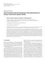
In Figure 3, we plot the rate regions when all link gains
are large (the link gain is 10 for all links). As mentioned in the
previous section, the AF strategy has the largest multiplexing
gain in the high SNR regime. We can see in Figure 3 that the
AF strategy achieves the largest sum rate.
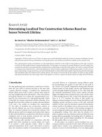
In Figures 4 and 5, we consider the case where relay 1 has
larger link gains than relay 2. In Figure 4, the link gains hA1
and hB1 are the same. In this case, HMC dominates all other
strategies. In Figure 5, the two link gains, hA1 and hB1 , are
not equal. In this case, HLC dominates HMC. HLC performs
better in this asymmetric case because of its ability to adjust
power between signals and utilize the beamforming gain.
When both relays are close to one of the terminals, PDF
has the best performance, as can be seen in Figure 6. The
reason is that both relays are able to decode reliably the
message from the closer terminal, and then they cooperatively forward the message to the other terminal using MIMO

techniques.
Figures 7 and 8 presents two scenarios in which DF
dominates all other transmission strategies. We remark that
DF is quite flexible in that it has many tunable parameters.
The case where both hA1 and hB2 are relatively large is shown
in Figure 7. Another case where hA1 and hA2 are larger than
hB1 and hB2 is shown in Figure 8. In both cases, DF is much
better than other strategies.
We can further summarize the numerical results in
Table 2. It is not supposed to be a precise description on the


10

EURASIP Journal on Wireless Communications and Networking
hA1 = 10 hB1 = 10 hA2 = 10 hB2 = 10

2

hA1 = 3 hB1 = 1 hA2 = 0.5 hB2 = 0.5

0.35

1.8

0.3

1.6
0.25

1.4

0.2

1

RB

RB

1.2

0.15

0.8
0.6

0.1

0.4
0.05

0.2
0

0

0.5

1

RA

1.5

0

2

0

0.05

0.1

0.15

0.2

0.25

0.3

0.35

0.4

0.45

RA

AF
DF
HMC

HLC
PDF
Outer bound

AF
DF
HMC

Figure 3: The achievable rate regions when all link gains are large.

HLC
PDF
Outer bound

Figure 5: The achievable rate regions when one relay has large link
gains (symmetric case).

hA1 = 2 hB1 = 2 hA2 = 0.5 hB2 = 0.5

0.7

hA1 = 5 hB1 = 1 hA2 = 5 hB2 = 1

0.4

0.6

0.35

0.5

0.3
0.4
RB

0.25
RB

0.3
0.2

0.15

0.1
0

0.2

0.1
0.05
0

0.1

0.2

0.3

0.4

0.5

0.6

0.7
0

RA
AF
DF
HMC

HLC
PDF
Outer bound

Figure 4: The achievable rate regions when one relay has large link
gains (symmetric case).

relative merits of the schemes. Instead, it provides a rough
guideline for easy selection of a suitable scheme. In the table,
“G” refers to “the channel condition is good” and “B” refers
to “the channel condition is bad.” We say that a channel is
good if its link gain is two to three times, or more, than the
link gain of a bad channel. When all the link gains are large,
we should use AF. In the case when one pair of the opposite

links of the network is good, whereas the other pair is weak,
DF provides larger throughput. If one of the relays is good
but the other relay is bad, HMC or HLC should be used.

0

0.1

0.2

0.3

0.4

0.5

0.6

0.7

RA
AF
DF
HMC

HLC
PDF
Outer bound

Figure 6: The achievable rate regions when both relays are close to

terminal A.

Table 1: Multiplexing gains of the transmission schemes in the high
SNR regime.
Scheme
Multiplexing gain

AF
2

HMC, HLC, DF
0.5

PDF
1.5

PDF scheme is the best one in the scenario where one of the
sources has large link gains but the other does not.


EURASIP Journal on Wireless Communications and Networking

7. Conclusion

hA1 = 10 hB1 = 1 hA2 = 1 hB2 = 10

0.5
0.45
0.4
0.35

RB

0.3
0.25
0.2
0.15
0.1
0.05
0

0

0.1

0.2

0.3

0.4

0.5

0.6

0.7

RA
AF
DF

HMC

HLC
PDF
Outer bound

Figure 7: The achievable rate regions and the outer bound.

hA1 = 5 hB1 = 0.5 hA2 = 2 hB2 = 1

0.35

11

0.3
0.25

We have devised several transmission strategies for the
TWTR network, each of which is derived from a mix-andmatch of several basic building blocks, namely, amplifyforward strategy, decode-forward strategy, and physicallayer network coding, and so forth. We can see from the
numerical examples that there is no single transmission
strategy that can dominate all other strategies under all
channel realizations. In other words, transmission strategy
should be tailor-made for a given environment. In this paper,
we have investigated the pros and cons of different building
blocks and demonstrated how they can be used to construct
transmission strategies for the TWTR network. We believe
that the idea can be applied to other relay networks as well.
While in this paper we only consider the case where
there are only two-relays, the ideas of our proposed schemes
can be applied to the case with more than two-relays. In

particular, AF and PDF can be directly implemented without
any change. As for DF, HMC, and HLC, the design may be
more complicated, since we have to determine which relay to
decode which source’s message. On the other hand, the idea
behind remains the same.
In our work, we have assumed that the channels are static.
When link gains are time varying, our result reveals that a
static strategy can only be suboptimal. To fully exploit the
available capacity of the network, adaptive strategies that can
switch between several modes are needed. How to determine
a good strategy based on channel state information is an
open problem. It is especially difficult if the switching is
based on local information only, and we leave it for future
work.

RB

0.2

Appendix

0.15

Proof of Theorem 4

0.1

The following information-theoretic argument shows that
any rate pair (RA , RB ) satisfying the conditions in Theorem 4
is achievable.

0.05
0

0

0.05

0.1

0.15

0.2

0.25

0.3

0.35

0.4

0.45

RA
AF
DF
HMC

HLC

PDF
Outer bound

Figure 8: The achievable rate regions and the outer bound.

Table 2: Performance guideline for the two-way two-relay network
in the medium SNR regime.
hA1
G
G
G
G

hB1
G
B
G
B

hA2
G
B
B
G

hB2
G
G
B
B

Scheme
AF
DF
HMC, HLC
PDF

Codebook Generation . For i = A, B, the common message
of terminal i is drawn uniformly in Mic
{1, 2, . . . , 22NRic }
and the private message from Mip
{1, 2, . . . , 22NRip }.
2NRic independent sequences
For i = A, B, we generate 2
of length N. In each sequence, the components are 2 × 1
vectors drawn independently with distribution N (0, Kic ).
Label the generated sequences by UN (mic ) for mic ∈ Mic .
i
Generate 22NRip independent sequences of length N, with
each component drawn independently with distribution
N (0, Kip ). Label the generated sequences by WN (mip ) for
i
mip ∈ Mip . Set
XiN mic , mip = Hi UN (mic ) + WN mip
i
i

.

(A.1)

By (56) and (57), with very high probability the power
constraints on node A and node B are satisfied.
There is a common codebook for relay 1 and relay 2. We
generate an array of codewords with 22NRAc rows and 22NRBc


12

EURASIP Journal on Wireless Communications and Networking

columns. The codewords have length N and each component
is drawn independently from N (0, 1). Label the codewords
N
by V0 (mAc , mBc ), for mAc ∈ MAc and mBc ∈ MBc .
For relay 1, we generate 22N(RA p +RAc RBc ) codewords,
indexed by mAp ∈ MAp , mAc ∈ MAc , mBc ∈ MBc , and
denoted by
N
X1 mAp , mAc , mBc .

(A.2)

Each of them is drawn independently with each component
N
generated from N (0, α1 P1 ). Let X1 (mAc , mBc , mAp ) be the
linear combination
N
N
α1 P1 V0 (mAc , mBc ) + X1 mAp , mAc , mBc .

(A.4)

for mB p ∈ MB p , mBc ∈ MBc , mAc ∈ MAc . The components of each codeword are generated independently from
N
N (0, α2 P2 ). Let X2 (mAc , mBc , mB p ) be
N
N
α2 P2 V0 (mAc , mBc ) + X2

mB p , mBc , mAc .

(A.5)

N
X2 (mAc , mBc , mB p )

The codeword
satisfies the power constraint of node 2 by the hypothesis that α2 + α2 < 1.
Encoding: For source node i ∈ {A, B}, to send the message
(mic , mip ), it sends XiN (mic , mip ) to the relays.
N
In the second stage, relay 1 and relay 2 transmit X1 (mAc ,
N
mBc , mAp ) and X2 (mAc , mBc , mB p ). The messages indicated
by is the estimated version of the original message.
Decoding: For i = 1, 2, the channel output at relay i is
hT HA UA (mAc )(t) + WA mAp (t)
Ai
(A.6)

+ hT HB UB (mBc (t)) + WB mB p (t) + Zi (t).
Bi
The receiver at relay 1 treats the signal component
hT HB WB (mB p )(t) as noise, and tries to decode mAc , mBc
B1
and mAp . It reduces to a MAC with two users, but three
independent messages; two messages from node A and
one message from node B. In order to decode these three
messages reliably, we need the requirement in (50). Likewise,
we have the requirement in (51) for correct decoding at node
2.
Relay 2 treats the signal component hT HA WA (mAp )(t)
A2
as noise, and tries to decode mAc , mBc and mB p . This can
be done with arbitrarily small error if the condition in (51)
holds.
In the second stage, terminal A receives
YA (t) =

α1 P1 hA1 + α2 P2 hA2 V0 (mAc , mBc )(t)
+ hA1 X1 mAp , mAc , mBc (t)
+ hA2 X2 mB p , mBc , mAc (t) + ZA (t).

RB p ≤ I X2 ; YA | X1 , V0 ,

(A.3)

N
Since α1 +α1 is strictly less than 1, X1 (mAc , mBc , mAp ) satisfies
the power constraint of node 1 with very high probability.

For relay 2, we generate 22N(RBc +RB p +RAc ) codewords,
labeled by
N
X2 mB p , mBc , mAc ,

Assuming that mAc = mAc and mAp = mAp , the channel is
equivalent to a two-user MAC with common information, in
which both users send mBc , and one of the users sends the
private message mB p . The decoding is done by typicality as
in [30, chapter 8], with the additional functionality of multiplexed coding. The decoder at terminal A searches for mBc
N
N
N
and mB p such that YA , V0 (mAc , mBc ), X1 (mAp , mAc , mBc )
N
and X2 (mB p , mBc , mAc ) are jointly typical. From the capacity
region of MAC with common information [30, page 102], we
obtain the following rate requirements

(A.7)

(A.8)
RB p + RBc ≤ I X1 , X2 , V0 ; YA ,
where I is the mutual information function. This gives the
conditions in (54) and (55).
Similarly, we have the conditions in (52) and (53) for
successful decoding in terminal B. This completes the proof
of Theorem 4.

Acknowledgment

This work is supported by a grant from the City University of
Hong Kong (Project no. SRG 7002386).

References
[1] E. C. van der Meulen, Transmission of information in a
T-terminals discrete memoryless channel, Ph.D. dissertation,
University of California, Berkeley, Calif, USA, June 1968.
[2] T. M. Cover and A. A. El Gamal, “Capacity theorems for the
relay channel,” IEEE Transactions on Information Theory, vol.
25, no. 5, pp. 572–584, 1979.
[3] A. Sendonaris, E. Erkip, and B. Aazhang, “User cooperation
diversity—part I: system description,” IEEE Transactions on
Communications, vol. 51, no. 11, pp. 1927–1938, 2003.
[4] J. N. Laneman, D. N. C. Tse, and G. W. Wornell, “Cooperative
diversity in wireless networks: efficient protocols and outage
behavior,” IEEE Transactions on Information Theory, vol. 50,
no. 12, pp. 3062–3080, 2004.
[5] C. E. Shannon, “Two-way communications channels,” in
Proceedings of the 4th Berkeley Symposium on Mathematical
Statistics and Probability, pp. 611–644, June 1961.
[6] R. Ahlswede, N. Cai, S.-Y. R. Li, and R. W. Yeung, “Network
information flow,” IEEE Transactions on Information Theory,
vol. 46, no. 4, pp. 1204–1216, 2000.
[7] B. Rankov and A. Wittneben, “Achievable rate regions for the
two-way relay channel,” in Proceedings of IEEE International
Symposium on Information Theory (ISIT ’06), pp. 1668–1672,
Seattle, Wash, USA, July 2006.
[8] P. Larsson, N. Johansson, and K.-E. Sunell, “Coded bidirectional relaying,” in Proceedings of the 63rd IEEE Vehicular
Technology Conference (VTC ’06), vol. 2, pp. 851–855, Melbourne, Australia, May-July 2006.
[9] S. J. Kim, P. Mitran, and V. Tarokh, “Performance bounds for

bidirectional coded cooperation protocols,” IEEE Transactions
on Information Theory, vol. 54, no. 11, pp. 5235–5241, 2008.
[10] D. Dash, A. Khoshnevis, and A. Sabharwal, “An achievable
rate region for a multiuser half-duplex two-way channel,” in
Proceedings of the 40th Asilomar Conference on Signals, Systems,


EURASIP Journal on Wireless Communications and Networking

[11]

[12]

[13]

[14]

[15]
[16]

[17]

[18]

[19]

[20]

[21]

[22]

[23]

[24]
[25]

[26]

[27]

and Computers (ACSSC ’06), pp. 707–711, Pacific Grove, Calif,
USA, October-November 2006.
C.-H. Liu and F. Xue, “Network coding for two-way relaying:
rate region, sum rate and opportunistic scheduling,” in Proceedings of IEEE International Conference on Communications
(ICC ’08), pp. 1044–1049, Beijing, China, May 2008.
I.-J. Baik and S.-Y. Chung, “Network coding for two-way relay
channels using lattices,” in Proceedings of IEEE International
Conference on Communications (ICC ’08), pp. 3898–3902,
Beijing, China, May 2008.
K. Narayanan, M. P. Wilson, and A. Sprintson, “Joint physical
layer coding and network coding for bi-directional relaying,”
in Proceedings of the 45th Annual Allerton Conference on Communication, Control, and Computing, University of Illinois,
June 2007.
W. Nam, S.-Y. Chung, and Y. H. Lee, “Capacity bounds for
two-way relay channels,” in Proceedings of International Zurich
Seminar on Communications (IZS ’08), pp. 144–147, Zurich,
Germany, March 2008.
B. Schein, Distributed coordination in network information
theory, Ph.D dissertation, MIT, Cambridge, Mass, USA, 2001.

F. Xue and S. Sandhu, “Cooperation in a half-duplex Gaussian
diamond relay channel,” IEEE Transactions on Information
Theory, vol. 53, no. 10, pp. 3806–3814, 2007.
G. Kramer, M. Gastpar, and P. Gupta, “Cooperative strategies
and capacity theorems for relay networks,” IEEE Transactions
on Information Theory, vol. 51, no. 9, pp. 3037–3063, 2005.
S. Zhang, S. C. Liew, and P. P. Lam, “Hot topic: physicallayer network coding,” in Proceedings of the 12th Annual
International Conference on Mobile Computing and Networking
(MOBICOM ’06), pp. 358–365, Los Angeles, Calif, USA,
September 2006.
S. Katti, S. Gollakota, and D. Katabi, “Embracing wireless
interference: analog network coding,” in Proceedings of the
ACM SIGCOMM Conference on Applications, Technologies,
Architectures, and Protocols for Computer Communications
(ACM SIGCOMM ’07), pp. 397–408, Kyoto, Japan, August
2007.
S. Zhang, S. C. Liew, and L. Lu, “Physical layer network
coding schemes over finite and infinite fields,” in Proceedings of
the IEEE Global Telecommunications Conference (GLOBECOM
’08), pp. 3784–3789, New Orleans, La, USA, NovemberDecember 2008.
B. K. Dey, S. Katti, S. Jaggi, D. Katabi, M. M´ dard, and S.
e
Shintre, ““Real” and “complex” network codes: promises and
challenges,” in Proceedings of the 4th Workshop on Network
Coding, Theory, and Applications (NetCod ’08), pp. 1–6, Hong
Kong, January 2008.
A. Høst-Madsen, “Capacity bounds for cooperative diversity,”
IEEE Transactions on Information Theory, vol. 52, no. 4, pp.
1522–1544, 2006.
E. Telatar, “Capacity of multi-antenna Gaussian channels,”

European Transactions on Telecommunications, vol. 10, no. 6,
pp. 585–595, 1999.
T. M. Cover and J. A. Thomas, Elements of Information Theory,
Wiley-Interscience, New York, NY, USA, 1991.
P. Hu, Cooperative strategies for Gaussian parallel relay networks, M.S. thesis, City University of Hong Kong, Hong Kong,
September 2009.
T. S. Han and K. Kobayashi, “A new achievable rate region for
the interference channel,” IEEE Transactions on Information
Theory, vol. 27, no. 1, pp. 49–60, 1981.
L. Zheng and D. N. C. Tse, “Diversity and multiplexing:
a fundamental tradeoff in multiple-antenna channels,” IEEE

13

Transactions on Information Theory, vol. 49, no. 5, pp. 1073–
1096, 2003.
[28] R. A. Horn and C. R. Johnson, Matrix Analysis, Cambridge
University Press, Cambridge, UK, 1985.
[29] M. A. Khojastepour, A. Sabharwal, and B. Aazhang, “Bounds
on achievable rates for general multiterminal networks with
practical constraints,” in Proceedings of the 2nd International
Conference on Information Processing in Sensor Networks (IPSN
’03), vol. 2634 of Lecture Notes in Computer Science, pp. 146–
161, Palo Alto, Calif, USA, 2003.
[30] G. Kramer, Topics in Multi-User Information Theory, vol. 4 of
Foundations and Trends in Communications and Information
Theory, NOW Publishers, 2007.