báo cáo hóa học:" Research Article A Semianalytical PDF of Downlink SINR for Femtocell Networks" pot

Hindawi Publishing Corporation
EURASIP Journal on Wireless Communications and Networking
Volume 2010, Article ID 256370, 9 pages
doi:10.1155/2010/256370
Research Article
A Semianalytical PDF of Downlink SINR for Femtocell Networks
Ki Won Sung,
1
Harald Haas,
2
and Stephen McLaughlin (EURASIP Member)
2
1
KTH Royal Institute of Technology, 164 40 Kista, Sweden
2
Institute for Digital Communications, The University of Edinburgh, King’s Buildings, Edinburgh EH9 3JL, UK
Correspondence should be addressed to Ki Won Sung,
Received 31 August 2009; Revised 4 January 2010; Accepted 17 February 2010
Academic Editor: Ozgur Oyman
Copyright © 2010 Ki Won Sung et al. This is an open access article distributed under the Creative Commons Attribution License,
which permits unrestricted use, distribution, and reproduction in any medium, provided the original work is properly cited.
This paper presents a derivation of the probability density function (PDF) of the signal-to-interference and noise ratio (SINR) for
the downlink of a cell in multicellular networks. The mathematical model considers uncoordinated locations and transmission
powers of base stations (BSs) which reflect accurately the deployment of randomly located femtocells in an indoor environment.
The derivation is semianalytical, in that the PDF is obtained by analysis and can be easily calculated by employing standard
numerical methods. Thus, it obviates the needfor time-consuming simulation efforts. The derivation of the PDF takes into account
practical propagation models including shadow fading. The effect of background noise is also considered. Numerical experiments
are performed assuming various environments and deployment scenarios to examine the performance of femtocell networks. The
results are compared with Monte Carlo simulations for verification purposes and show good agreement.
1. Introduction
Signal-to-interference and noise ratio (SINR) is one of the

most important performance measures in cellular systems.
Its probability distribution plays an important role for
system performance evaluation, radio resource management,
and radio network planning. With an accurate probability
density function (PDF) of SINR, the capacity and coverage
of a system can be easily predicted, which otherwise should
rely on complicated and time-consuming simulations.
There have been various approaches to investigate the
statistical characteristics of received signal and interference.
The other-cell interference statistics for the uplink of code
division multiple access (CDMA) system was investigated in
[1], where the ratio of other-cell to own-cell interference was
presented. The result was extended to both the uplink and
the downlink of general cellular systems by [2]. In [3], the
second-order statistics of SIR for a mobile station (MS) were
investigated. In [4, 5], the prediction of coverage probability
was addressed which is imperative in the radio network
planning process. The probability that SINR goes below
a certain threshold, which is termed outage probability,
is another performance measure that has been extensively
explored. The derivation of the outage probability can be
found in [6–8] and references therein.
While most of the contributions have focused on a
particular performance measure such as coverage probability
or outage probability, an explicit derivation of the probability
distribution for signal and interference has also been investi-
gated [9, 10]. In [9], a PDF of adjacent channel interference
(ACI) was derived in the uplink of cellular system. A PDF of
SIR in an ad hoc system was studied in [10] assuming single
transmitter and receiver pair.

In this paper, we derive the PDF of the SINR for the
downlink of a cell area in a semianalytical fashion. A practical
propagation loss model combined with shadow fading is
considered in the derivation of the PDF. We also consider
background noise in the derivation, which is often ignored
in the references. Uncoordinated locations and transmission
powers of interfering base stations (BSs) are considered in
the model to take into account the deployment of femtocells
(or home BSs) [11] in an indoor environment. It has been
suggested that femto BSs can significantly improve system
spectral efficiency by up to a factor of five [12]. It has
also been found that in closed-access femtocell networks
macrocell MSs in close vicinity to a femtocell greatly suffer
from high interference and that such macrocell MSs cause
destructive interference to femtocell BSs [13]. Thus, an
accurate model for the probability distribution of the SINR
2 EURASIP Journal on Wireless Communications and Networking
assuming an uncoordinated placement of indoor BSs can be
vital for further system improvements. In spite of the recent
efforts for the performance evaluation of femtocells, most
of the works relied on system simulation experiments [12–
17]. To the best of our knowledge, the PDF of SINR for the
outlined conditions and environment has not been derived
before.
Since shadow fading is generally considered to follow a
log-normal distribution, the PDF of the sum of log-normal
RVs should be provided as a first step in the derivation of
the SINR distribution. During the last few decades numerous
approximations have been proposed to obtain the PDF of
the sum of log-normal RVs since the exact closed-form

expression is still unknown [18–23]. So far, no method offers
significant advantages over another [18], and sometimes a
tradeoff exists between the accuracy of the approximation
and the computational complexity. We adopt two methods
of approximation proposed by Fenton and Wilkinson [19]
and Mehta et al. [20] which provide a good balance between
accuracy and complexity. The performance of both methods
is examined in various environments and a guideline is
provided for choosing one of the methods.
The derivation of SINR distribution in this paper is semi-
analytical in the sense that the PDF can be easily calculated by
applying standard numerical methods to equations obtained
from analysis. Numerical experiments are performed to
investigate the effects of standard deviation of shadow fading,
the number of interfering BSs, wall penetration loss, and
transmission powers of BSs. The results obtained are also
validated by comparison with Monte Carlo simulations.
The paper is organised as follows. In Section 2, the PDF
of the downlink SINR is derived. Numerical experiments
are performed in various environments and the results
are compared with Monte Carlo simulations in Section 3.
Finally, the conclusions are provided in Section 4.
2. Derivation of the PDF of Downlink SINR
The derivation of the PDF of downlink SINR is divided into
two parts. First, the SINR of an arbitrary MS is expressed
depending on its location in Section 2.1. Methods of approx-
imating the sum probability distribution of log-normal RVs
are discussed and adopted in the SINR derivation. Second,
the PDF of SINR unconditional on the location of the MS is
derived in Section 2.2.

2.1. Locat ion-Dependent SINR. Let us consider a femtocell
which will be termed the cell of interest (CoI). The CoI
is assumed to be circular with a cell radius R. We assume
the MSs in the CoI to be uniformly distributed in the cell
area. An arbitrary MS m is considered whose location is
(r
m
, θ
m
), where 0 ≤ r
m
≤ R and 0 ≤ θ
m
≤ 2π.The
MS m receives interference from L BSs that are a mixture
of femto and macro-BSs. The network is modelled using
polar coordinates where the BS of the CoI is located at the
center and the location of the jth interfering BS is denoted by
(r
b
(j), θ
b
(j)). In a practical deployment of femtocell systems,
the placement of BSs in a random and uncoordinated fashion
is unavoidable and may generate high interference scenarios
and dead spots particularly in an indoor environment.
Let P
t
s
be the transmission power of the BS in the CoI. It

is attenuated by path loss and shadow fading. Let X
s
be the
RV which models the shadow fading. It is generally assumed
that X
s
follows a Gaussian distribution with zero mean and
variance σ
2
X
s
in dB. Thus the received signal power at the MS
m from the serving BS, P
r
s
,isdenotedby
P
r
s
= P
t
s
G
b
G
m
C
s
r
m

−α
s
exp

βX
s

,
(1)
where G
b
and G
m
are antenna gains of the BS and the MS,
respectively, C
s
is constant of path loss in the CoI, α
s
is path
loss exponent of CoI, and β
= ln(10)/10. The ln(·)denotes
natural logarithm. P
r
s
can be rewritten as follows:
P
r
s
= exp


ln

P
t
s
G
b
G
m
C
s

−
α
s
ln r
m
+ βX
s

.
(2)
Note that an RV Y
= exp(V) follows a log-normal distri-
bution if V is a Gaussian distributed RV. Thus, P
r
s
follows a
log-normal distribution conditioned on the location of MS
m. The PDF of P

r
s
is given by
f
P
r
s
(
z
| r
m
, θ
m
)
=
1
zσ
s
√
2π
exp

−

ln z −μ
s

2
2σ
2

s

,
(3)
where μ
s
= ln(P
t
s
G
b
G
m
C
s
) −α
s
ln r
m
and σ
2
s
= β
2
σ
2
X
s
.
Let I

r
j
be the received interference power from the jth
interfering BS. By denoting P
t
j
as the transmission power
from the jth BS, I
r
j
results in
I
r
j
= P
t
j
G
b
G
m
C
j
d
mb

j

−α
j

exp

βX
j

,(4)
where C
j
and α
j
are the path loss constant and exponent,
respectively, on the link between the jth BS and MS m,and
X
j
is a Gaussian RV for shadow fading with zero mean and
variance σ
2
X
j
on the link between the jth BS and MS m.
Note that the transmission power of each interfering BS can
be different since an uncoordinated femtocell deployment is
considered. Path loss parameters and standard deviation of
shadow fading can also be different in each BS in practical
systems. The distance between MS m and the jth interfering
BS is d
mb
(j), which is obtained from
d
mb


j

=

r
2
m
+ r
b

j

2
−2r
m
r
b

j

cos

θ
m
−θ
b

j



1/2
.
(5)
In a similar fashion to P
r
s
, I
r
j
follows a log-normal distribu-
tion with PDF given by
f
I
r
j
(
z
| r
m
, θ
m
)
=
1
zσ
j
√
2π
exp

⎡
⎢
⎣
−

ln z −μ
j

2
2σ
2
j
⎤
⎥
⎦
,
(6)
where μ
j
= ln(P
t
j
G
b
G
m
C
j
) −α
j

ln d
mb
(j)andσ
2
j
= β
2
σ
2
X
j
.
Background noise can be regarded as a constant value by
assuming the constant noise figure and the noise tempera-
ture. Let N
bg
be the background noise power at MS m,given
by
N
bg
= kTWϕ,
(7)
EURASIP Journal on Wireless Communications and Networking 3
where k is the Boltzmann constant, T is the ambient
temperature in Kelvin, W is the channel bandwidth, and
ϕ is the noise figure of the MS. In order to make N
bg
mathematically tractable, we introduce an auxiliary Gaussian
RV X
n

with zero mean and zero variance so that N
bg
can
betreatedaslog-normalRVwithparametersofμ
n
=
ln(kTWϕ)andσ
n
= 0. Note that N
bg
has a constant value,
and this is accounted for by the fact that the defined RV
has zero variance. This particular definition is useful for the
determination of the final PDF. By introducing X
n
, N
bg
can
be rewritten as follows:
N
bg
= kTWϕexp
(
X
n
)
= exp

ln


kTWϕ

+ X
n

.
(8)
Let us consider a system with no interference arising from
the serving cell such as an OFDMA or a TDMA system. The
downlinkSINRofMSm is denoted by γ
m
, which is given by
γ
m
=
P
r
s

L
j
=1
I
r
j
+ N
bg
=
P
r

s
Υ
.
(9)
In (9), Υ denotes the sum of the interference powers and
the background noise power. Since all of I
r
j
and N
bg
are log-
normally distributed, Υ is the sum of L + 1 log-normal RVs.
Note that the exact closed-form expression is not known for
the PDF of the sum of log-normal RVs. The most widely
accepted approximation approach is to assume that the sum
of log-normal RVs follows a log-normal distribution. Various
methods have been proposed to find out parameters of the
distribution [19–21].
Let Y
1
, , Y
M
be M independent but not necessarily
identicallog-normalRVs,whereY
j
= exp(V
j
)andV
j
is a Gaussian distributed RV with mean μ

V
j
and variance
σ
2
V
j
. The sum of M RVsisdenotedbyY such that Y =

M
j
=1
Y
j
. Approximations assume that Y follows a log-
normal distribution with parameters μ
V
and σ
2
V
.
The Fenton and Wilkinson (FW) method [19]isoneof
the most frequently adopted approximations in literature. It
obtains μ
V
and σ
2
V
by assuming that the first and second
moments of Y match the sum of the moments of Y

j
.It
should be noted that the FW method is the only approximate
method that provides a closed-form expression of μ
V
and σ
2
V
[20]. Let us denote μ
n
as μ
L+1
and σ
n
as σ
L+1
.From[19], the
PDF of Υ conditioned on the location of MS m is given as
follows:
f
Υ
(
z
| r
m
, θ
m
)
=
1

zσ
Υ
√
2π
exp

−

ln z −μ
Υ

2
2σ
2
Υ

,
(10)
where μ
Υ
and σ
2
Υ
are given by
σ
2
Υ
= ln
⎡
⎢

⎣

L+1
j=1
exp

2μ
j
+ σ
2
j

exp

σ
2
j

−
1



L+1
j
=1
exp

μ
j

+ σ
2
j
/2

2
+1
⎤
⎥
⎦
,
μ
Υ
= ln
⎡
⎣
L+1

j=1
exp

μ
j
+
σ
2
j
2

⎤

⎦
−
σ
2
Υ
2
.
(11)
In spite of its simplicity, the accuracy of the FW method
suffersathighvaluesofσ
2
V
j
. This means that the method
may break down when an MS experiences a large standard
deviation of shadow fading from interfering BSs. Thus, we
adopt another method of approximating the sum of log-
normal RVs which gives a more accurate result at a cost of
increased computational complexity.
The method proposed in [20], which is called MWMZ
method in this paper after the initials of authors, exploits the
property of the moment-generating function (MGF) that the
product of MGFs of independent RVs equals to the MGF of
the sum of RVs. The MGF of RV Y is defined as
Ψ
Y
(
s
)
=


∞
0
exp

−
sy

f
Y

y

dy.
(12)
By the property of MGF,
Ψ
Y
(
s
)
=
M

j=1
Ψ
Y
j
(
s

)
.
(13)
While the closed-form expression for the MGF of log-
normal distribution is not available, a series expansion based
on Gauss-Hermite integration was employed in [20]to
approximate the MGF. For a real coefficient s, the MGF of
the log-normal RV Y is given by

Ψ
Y

s; μ
V
, σ
V

Δ
=
M

j=1
w
j
√
π
exp

−
s exp


√
2σ
V
a
j
+ μ
V

,
(14)
where w
j
and a
j
are weights and abscissas of the Gauss-
Hermite series which can be found in [24,Table25.10]. From
(13), a system of two nonlinear equations can be set up with
two real and positive coefficients s
1
and s
2
as follows:
M

j=1
w
j
√
π

exp

−
s
i
exp

√
2σ
V
a
j
+ μ
V

=
M

j=1

Ψ
Y
j

s
i
; μ
V
j
, σ

V
j

, i = 1, 2.
(15)
The variables to be solved by (15)areμ
V
and σ
V
. The right-
hand side of (15) is a constant value which can be calculated
with known parameters.
By employing (15), μ
Υ
and σ
2
Υ
in (10)canbeeffectively
obtained by standard numerical methods such as the func-
tion “fsolve” in Matlab. The coefficient s
= (s
1
, s
2
) adjusts
weight of penalty for inaccuracy of the PDF. Increasing s
imposes more penalty for errors in the head portion of the
PDF of Y, whereas smaller s penalises errors in the tail
portion. Thus, smaller s is recommended if one is interested
in the PDF of poor SINR region, while larger s should be used

to examine statistics of higher SINR.
As shown in (3), the received signal power, P
r
s
,fol-
lows a log-normal distribution. The sum of the received
interference and the background noise power, Υ, was also
approximated as a log-normal RV. Thus, the SINR of the MS
m, γ
m
, is the ratio of two log-normal RVs, which also follows
4 EURASIP Journal on Wireless Communications and Networking
Cell of interest
(0,0)
MS m
Cell j
(r
b
(j), θ
b
(j))
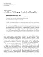
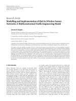
Figure 1: Locations of the CoI and the interfering BSs.
Table 1: Simulation parameters.
Parameter Value
Cell radius 50 m
Path loss exponent 3.68
Path loss constant 43.8 dB
Center frequency 5.25 GHz
Channel bandwidth 10 MHz
MS noise figure 7 dB

BS transmission power 20 dBm
BS antenna gain 3 dBi
MS antenna gain 0 dBi
Number of interfering cells 6
Frequency reuse factor 1
Table 2: Kullback-Leibler Distance between the simulation and the
analysis (
×10
−4
).
σ
X
s
and σ
X
j
[dB] FW method MWMZ method
3 6.00 6.98
4 3.66 4.34
5 11.32 6.05
6 35.70 8.81
7 90.50 12.29
8 186.87 16.24
9 324.10 21.23
10 489.04 26.13
a log-normal distribution. From (3)and(10), the PDF of γ
m
is shown as
f
γ

m
(
z
| r
m
, θ
m
)
=
1
zσ
γ
m
√
2π
exp
⎡
⎢
⎣
−

ln z −μ
γ
m

2
2σ
2
γ
m

⎤
⎥
⎦
,
(16)
where μ
γ
m
= μ
s
−μ
Υ
and σ
2
γ
m
= σ
2
s
+ σ
2
Υ
.
2.2. The PDF of Downlink SINR in a Cell. Up to this
point, the PDF of the downlink SINR has been derived
conditionally on the location of the MS m.Letusdenote
the location of MS m by ρ. Since it is assumed that MSs are
uniformly distributed within a circular area, the PDF of ρ,
f
ρ

(r
m
, θ
m
), is as follows:
f
ρ
(
r
m
, θ
m
)
=
r
m
πR
2
.
(17)
From (16)and(17), the joint distribution of the SINR and
the MS location is
f
γ
m
,ρ
(
z, r
m
, θ

m
)
= f
γ
m
(
z
| r
m
, θ
m
)
f
ρ
(
r
m
, θ
m
)
=
r
m
zσ
γ
m
R
2
√
2π

3
exp
⎡
⎢
⎣
−

ln z −μ
γ
m

2
2σ
2
γ
m
⎤
⎥
⎦
.
(18)
Let γ be the RV of the downlink SINR of an MS in an
arbitrary location within a circular cell area. The PDF of γ
can be obtained by integrating f
γ
m
,ρ
(z, r
m
, θ

m
)overr
m
and
θ
m
. Thus, we get
f
γ
(
z
)
=

R
0

2π
0
r
m
zσ
γ
m
R
2
√
2π
3
exp

⎡
⎢
⎣
−

ln z −μ
γ
m

2
2σ
2
γ
m
⎤
⎥
⎦
dθ
m
dr
m
.
(19)
Note that μ
γ
m
in (19) is a function of (r
m
, θ
m

). We employ
numerical integration methods to obtain the final PDF.
3. Numerical Results
The PDF of downlink SINR derived in (19) is calculated
numerically and compared with a Monte Carlo simulation
result in order to validate the analysis. We consider the
nonline of sight (NLOS) indoor environment at 5.25 GHz as
specified in [25, page 19] to be the basic environment for the
comparison. The path loss formula is given as follows:
PL
(
d
)
= 43.8+36.8log
10

d
d
0

,
(20)
where d
0
is a reference distance in the far field. The interfer-
ing BSs are assumed to be femto BSs located on the same
floor of a building throughout the experiments. However,
interference scenarios such as femto BSs in different floors
or outdoor macro-BSs can be easily examined by employing
appropriate path loss models. The basic parameters used for

the comparison are summarised in Tabl e 1.
We assume that all interfering BSs are located at the
same distance from the serving BS as shown in Figure 1.
Cellsareassumedtooverlapeachothertoconsideradense
deployment of the femto BSs. Although it is unlikely that
the interfering BSs are in regular shapes in practical deploy-
ments, it is useful to consider this topology for examining
the effects of parameters such as standard deviation of
shadow fading, the number of BSs, wall penetration loss, and
transmission power of BSs. It should be emphasised that the
EURASIP Journal on Wireless Communications and Networking 5
0
0.005
0.01
0.015
0.02
0.025
0.03
0.035
0.04
0.045
0.05
−20 −10
010203040
Probability density function
Downlink SINR (dB)
Simulation
FW method
MWMZ method
(a) PDF of the downlink SINR

0
0.1
0.2
0.3
0.4
0.5
0.6
0.7
0.8
0.9
1
−20 −10
010203040
Cumulative distribution function
Downlink SINR (dB)
Simulation
FW method
MWMZ method
(b) CDF of the downlink SINR
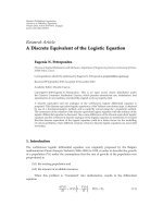
Figure 2: A comparison of the PDF and CDF obtained by the analysis with the result of Monte Carlo simulation (σ
X
s
= σ
X
j
= 3.5 dB).
0.02
0.022
0.024
0.026

0.028
0.03
0.032
0.034
0.036
0.038
0.04
−8.4 −8.2
−8 −7.8 −7.6 −7.4 −7.2 −7 −6.8 −6.6
Cumulative distribution function
Downlink SINR (dB)
Simulation
s
= (0.01,0.05)
s
= (0.001,0.005)
s
= (0.0001,0.0005)
(a) Tail portion of the CDF
0.97
0.971
0.972
0.973
0.974
0.975
0.976
0.977
0.978
0.979
0.98

27 27.5
28 28.52929.530
Cumulative distribution function
Downlink SINR (dB)
Simulation
s
= (0.01,0.05)
s
= (0.001,0.005)
s
= (0.0001,0.0005)
(b) Head portion of the CDF
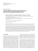
Figure 3: Impact of s on the performance of MWMZ method: tail and head portions of CDF (σ
X
s
= σ
X
j
= 3.5 dB).
PDF derived in Section 2 can effectively take into account
irregular locations and transmission powers of BSs.
The result of the comparison is illustrated in Figure 2
where the PDFs derived by FW and MWMZ methods
are compared with the Monte Carlo simulation result
in Figure 2(a) and the cumulative distribution functions
(CDFs) of the PDFs are depicted in Figure 2(b). The standard
deviation of shadow fading, σ
X
s
and σ

X
j
, is considered to be
3.5 dB since it represents a typical value in an indoor office
environment according to the measurement results in [25].
It is observed that the numerically obtained PDFs from both
of the methods are in good agreement with the Monte Carlo
simulation.
The impact of the parameter s on the performance of
MWMZ method is shown in Figure 3 where the tail portion
of the CDF (low SINR region) is depicted in Figure 3(a) and
the head portion of the CDF (high SINR regime) is illustrated
in Figure 3(b).Smallers tends to give more accurate match in
low SINR region while resulting in larger error in high SINR
region. s
= (0.01, 0.05) is chosen in the experiments since
it brings about relatively small difference from simulations
throughout the whole SINR region.
6 EURASIP Journal on Wireless Communications and Networking
0
0.1
0.2
0.3
0.4
0.5
0.6
0.7
0.8
0.9
1

−20 −10
010203040
Cumulative distribution function
Downlink SINR (dB)
Simulation
FW method
MWMZ method
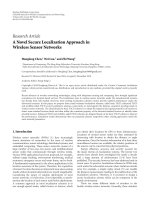
Figure 4: A comparison of the CDF obtained by the analysis with
the result of Monte Carlo simulation (σ
X
s
= σ
X
j
= 8.0 dB).
0
1
2
3
4
5
6
×10
−4
236183660
Kullback-Leibler distance
Number of interfering BSs
FW method
MWMZ method
Figure 5: Kullback-Leibler Distance between simulation and

analysis (σ
X
s
= σ
X
j
= 3.5 dB).
Figure 4 shows the CDFs when the standard deviation of
shadow fading is 8.0 dB. While the SINR obtained by MWMZ
method is still in good agreement with the simulation result,
the difference between the analysis and the simulation is
apparent in case of FW method. It means that FW method
cannot be used in an environment where high shadow fading
is experienced by MSs. In order to quantify the effect of
shadow fading standard deviation, we introduce Kullback-
Leibler Distance (KLD) which is a measure of divergence
0
0.1
0.2
0.3
0.4
0.5
0.6
0.7
0.8
0.9
1
−20 −10
0 10203040
Cumulative distribution function

Downlink SINR (dB)
Ω
j
= 0dB
Ω
j
= 5dB
Ω
j
= 10 dB
Ω
j
= 15 dB
Figure 6: Effect of wall penetration loss on CDF of SINR (FW
method, σ
X
s
= σ
X
j
= 3.5 dB).
0
0.1
0.2
0.3
0.4
0.5
0.6
0.7
0.8

0.9
1
−20 −10
0 10203040
Cumulative distribution function
Downlink SINR (dB)
Scenario 1
Scenario 2
Scenario 3
Scenario 4
Figure 7: Effect of different wall penetration losses on CDF of SINR
(FW method, σ
X
s
= σ
X
j
= 3.5 dB).
between two probability distributions [26]. For the two PDFs
p(x)andq(x)theKLDisdefinedas
D

pq

=

p
(
x
)

log
2
p
(
x
)
q
(
x
)
dx.
(21)
The KLD is a nonnegative entity which measures the
difference of the estimated distribution q(x) from the real
distribution p(x) in a statistical sense. It becomes zero if and
only if p(x)
= q(x). Ta b le 2 presents the KLD for various
standard deviations of shadow fading by assuming that the
simulation results represent the true PDFs of SINR. It is
shown in the table that the KLD of FW method soars when
EURASIP Journal on Wireless Communications and Networking 7
0
0.1
0.2
0.3
0.4
0.5
0.6
0.7
0.8

0.9
1
−20 −10
0102030
Cumulative distribution function
Downlink SINR (dB)
Scenario 5
Scenario 6
Scenario 7
Scenario 8
Figure 8: CDF of SINR with uncoordinated BS transmission power
(FW method, σ
X
s
= σ
X
j
= 3.5 dB).
0
0.1
0.2
0.3
0.4
0.5
0.6
0.7
0.8
0.9
1
−10 0

10 20 30
Cumulative distribution function
Downlink SINR (dB)
P
t
s
= P
t
j
= 10 dBm
P
t
s
= P
t
j
= 20 dBm
P
t
s
= P
t
j
= 30 dBm
Figure 9: Effect of BS transmission power and background noise
on CDF of SINR (FW method, σ
X
s
= σ
X

j
= 3.5 dB).
the standard deviation of shadow fading is higher than
6 dB. This implies that the range of standard deviation in
whichFWmethodcanbeadoptedisbetween3dBand
6 dB, which is a typical range of shadow fading in an in-
building environment [14, 25]. On the contrary, the MWMZ
method maintains an acceptable level of the KLD even for
the high shadow fading standard deviation. FW method is
preferred if both of the methods are applicable due to its
simplicity.
The effect of the number of interfering BSs is examined
in Figure 5. It is known that the sum of log-normal RVs is
not accurately approximated by a log-normal distribution as
the number of summands increases [22]. This means that
the derived SINR may not be accurate for a large number of
interfering BSs. Figure 5 shows the KLD of FW and MWMZ
methods compared to simulation results when L is between
2 and 60. An impairment in the accuracy is not observed as
L increases, which means that the derivation of SINR in this
paper is useful for the practical range of interfering BSs in the
downlink of cellular systems.
The numerical results so far have focused on the
verification of the derived PDF. Now we investigate the
performance of femtocell network in various environments.
An important observation in Figure 2 is that the probability
of the SINR below 2.2 dB (a typical threshold for binary
phase shift keying (BPSK) to achieve reasonable BER per-
formance [27]) is about 0.38 for the parameters in Ta bl e 1.
In other words, the outage probability is around 38%. This

means that a dense deployment of femtocells in a building
results in unacceptable outage, unless intelligent interference
avoidance and interference mitigation techniques are put in
place.
Clearly isolation of a cell by wall penetration loss is
an inherent property of indoor femtocell networks which
can be utilised as a means of interference mitigation. Let
Ω
j
be the wall penetration loss between the CoI and the
interfering BS j. The effect of Ω
j
is examined in Figure 6
where Ω
j
is assumed to be identical for all interfering BSs.
It is shown that Ω
j
has significant impact on the SINR of
the femtocell. The outage probability drops to 3.7% when
Ω
j
= 10 dB and to 0.5% when Ω
j
= 15 dB. This result
implies that the implementation of the femtocell network is
viable without complicated interference mitigation method
if the wall isolation between BSs is provided.
In Figure 7,different wall losses, Ω
j

, are considered. We
examine the following scenarios:
(i) scenario 1: Ω
1
=···=Ω
6
= 0dB,
(ii) scenario 2: Ω
1
=···=Ω
5
= 0dBandΩ
6
= 15 dB,
(iii) scenario 3: Ω
1
=···=Ω
6
= 15 dB,
(iv) scenario 4: Ω
1
=···=Ω
5
= 15 dB and Ω
6
= 0dB.
It is shown that scenarios 1 and 2 give similar perfor-
mance. This means that the isolation from one or few BSs
does not result in the performance improvement when the
CoI is not protected from the majority of interfering BSs. On

the contrary, a considerable difference is observed between
scenarios 3 and 4. Significant degradation in the SINR is
caused by one BS which is not isolated by the wall.
Similar behaviours are observed in Figure 8 where dif-
ferent BS transmission powers are considered. The effect of
the uncoordinated power is examined by considering the
following scenarios where P
t
s
= 20 dBm:
(i) scenario 5: P
t
1
=···=P
t
6
= 20 dBm,
(ii) scenario 6: P
t
1
= P
t
2
= P
t
3
= 30 dBm and P
t
4
= P

t
5
=
P
t
6
= 10 dBm,
8 EURASIP Journal on Wireless Communications and Networking
(iii) scenario 7: P
t
1
= P
t
2
= P
t
3
= 25 dBm and P
t
4
= P
t
5
=
P
t
6
= 20 dBm,
(iv) scenario 8: P
t

1
= 30 dBm and P
t
2
= ··· = P
t
6
=
20 dBm.
Figure 8 shows the CDFs of SINR by FW method with
the assumption that Ω
j
= 0dB ∀j. It is observed that
scenario 6 results in the worst SINR. This means that the
higher transmission powers of a few BSs result in significantly
decreased SINR. However, reduced transmission power in
only a subset of neighbouring BSs does not necessarily
improve the SINR because the predominant interference
largely depends on the BSs which use high transmission
powers. A similar trend is shown when comparing scenario 7
and scenario 8. The SINR performance is worse in scenario 8
than in scenario 7 for the same reason.
Finally, the effects of the BSs transmission power and
the background noise are shown in Figure 9. If the transmit
power drops below a certain level, a change in the PDF
can be observed. For 10 dBm transmit power, for example,
a noticeable impairment of the SINR can be seen. This is
because the noise power remains the same regardless of the
transmission power. In the case of increased transmission
power, however, little change in the SINR distribution is

observed. This means that the SINR is already interference
limited with a transmission power of 20 dBm. Thus, the
increase in the transmit power of BSs does not result in an
improvement as expected.
4. Conclusion
In this paper, the PDF of the SINR for the downlink
of a cell has been derived in a semianalytical fashion.
It models an uncoordinated deployment of BSs which is
particularly useful for the analysis of femtocells in an indoor
environment. A practical propagation model including log-
normal shadow fading is considered in the derivation
of the PDF. The PDF presented in this paper has been
obtained through analysis and calculated through standard
numerical methods. The comparison with Monte Carlo
simulation shows a good agreement, which indicates that
the semianalytical PDF obviates the need for complicated
and time-consuming simulations. The results also provide
some insights into the performance of the indoor femtocells
with universal frequency reuse. First, significant outage can
be expected for a scenario where femto BSs are densely
deployed in an in-building environment. This highlights that
interference avoidance and mitigation techniques are needed.
The isolation offered by wall penetration loss is an attractive
solution to cope with the interference. Second, the SINR can
be worsened by uncoordinated transmission powers of BSs.
Thus, a coordination of BSs transmission power is needed to
prevent a significant decrease in SINR.
Acknowledgment
This work was supported by the National Research Foun-
dation of Korea, Grant funded by the Korean Government

(NRF-2007-357-D00165).
References
[1] A. J. Viterbi, A. M. Viterbi, and E. Zehavi, “Other-cell interfer-
ence in cellular power-controlled CDMA,” IEEE Transactions
on Communications, vol. 42, no. 4, pp. 1501–1504, 1994.
[2] M. Zorzi, “On the analytical computation of the interference
statistics with applications to the performance evaluation of
mobile radio systems,” IEEE Transactions on Communications,
vol. 45, no. 1, pp. 103–109, 1997.
[3] F. Graziosi, L. Fuciarelli, and F. Santucci, “Second order
statistics of the SIR for cellular mobile networks in the
presence of correlated co-channel interferers,” in Proceedings
of the 53th IEEE Vehicular Technolog y Conference (VTC ’01),
pp. 2499–2503, Rhodes, Greece, May 2001.
[4] V. Koshi, “Coverage uncertainty and reliability estimation for
microcellular radio network planning,” in Proceedings of the
51th IEEE Vehicular Technology Conference (VTC ’00), pp. 468–
472, Tokyo, Japan, May 2000.
[5] D. Stachle, “An analytic method for coverage prediction in
the UMTS radio network planning process,” in Proceedings of
the 61th IEEE Vehicular Technology Conference (VTC ’05),pp.
1945–1949, Stockholm, Sweden, May-June 2005.
[6] M. Pratesi, F. Santucci, F. Graziosi, and M. Ruggieri, “Outage
analysis in mobile radio systems with generically correlated
log-normal interferers,” IEEE Transactions on Communica-
tions, vol. 48, no. 3, pp. 381–385, 2000.
[7] M. Pratesi, F. Santucci, and F. Graziosi, “Generalized moment
matching for the linear combination of lognormal RVs:
application to outage analysis in wireless systems,” IEEE
Transactions on Wireless Communications,vol.5,no.5,pp.

1122–1132, 2006.
[8] F. Berggren and S. B. Slimane, “A simple bound on the outage
probability with lognormally distributed interferers,” IEEE
Communications Letters, vol. 8, no. 5, pp. 271–273, 2004.
[9] H. Haas and S. McLaughlin, “A derivation of the PDF of
adjacent channel interference in a cellular system,” IEEE
Communications Letters, vol. 8, no. 2, pp. 102–104, 2004.
[10]A.Mudesir,M.Bode,K.W.Sung,andH.Haas,“Analytical
SIR for self-organizing wireless networks,” EURASIP Journal
on Wireless Communications and Networking, vol. 2009, Article
ID 912018, 8 pages, 2009.
[11] V. Chandrasekhar, J. G. Andrews, and A. Gatherer, “Femtocell
networks: a survey,” IEEE Communications Magazine, vol. 46,
no. 9, pp. 59–67, 2008.
[12] Z. Bharucha and H. Haas, “Application of the TDD underlay
concept to home nodeB scenario,” in Proceedings of the 7th
IEEE Vehicular Technology Conference (VTC ’08), pp. 56–60,
Singapore, May 2008.
[13] Z. Bharucha, I.
´
Cosovi
´
c, H. Haas, and G. Auer, “Throughput
enhancement through femto-cell deployment,” in Proceedings
of the IEEE 7th International Workshop on Multi-Carrier
Systems & Solutions (MC-SS ’09), pp. 311–319, Herrsching,
Germany, May 2009.
[14] H. Claussen, “Performance of macro—and co-channel fem-
tocells in a hierarchical cell structure,” in Proceedings of the
18th IEEE International Symposium on Personal, Indoor and

Mobile Radio Communications (PIMRC ’07), Athens, Greece,
November 2007.
[15] J. Espino and J. Markendahl, “Analysis of macro—femtocell
interference and implications for spectrum allocation,” in
Proceedings of the 20th IEEE International Symposium on
Personal, Indoor and Mobile Radio Communications (PIMRC
’09), pp. 13–16, Tokyo, Japan, September 2009.
EURASIP Journal on Wireless Communications and Networking 9
[16] A.Valcarce,G.D.L.Roche,A.J
¨
uttner,D.Lopez-Perez,andJ.
Zhang, “Applying FDTD to the coverage prediction of wiMAX
femtocells,” Eurasip Journal on Wireless Communications and
Networking, vol. 2009, Article ID 308606, 13 pages, 2009.
[17] M. Yavuz, F. Meshkati, S. Nanda, et al., “Interference manage-
ment and performance analysis of UMTS/HSPA+ femtocells,”
IEEE Communications Magazine, vol. 47, no. 9, pp. 102–109,
2009.
[18] N. C. Beaulieu and Q. Xie, “An optimal lognormal approxi-
mation to lognormal sum distributions,” IEEE Transactions on
Vehicular Technology, vol. 53, no. 2, pp. 479–489, 2004.
[19] L. F. Fenton, “The sum of log-normal probability distributions
in scatter transmission systems,” IRE Transactions on Commu-
nications Systems, vol. 8, no. 1, pp. 57–67, 1960.
[20] N. B. Mehta, J. Wu, A. F. Molisch, and J. Zhang, “Approxi-
mating a sum of random variables with a lognormal,” IEEE
Transactions on Wireless Communications,vol.6,no.7,pp.
2690–2699, 2007.
[21] S. C. Schwartz and Y. S. Yeh, “On the distribution function and
moments of power sums with log-normal components,” The

Bell System Technical Journal, vol. 61, no. 7, pp. 1441–1462,
1982.
[22] S. S. Szyszkowicz and H. Yanikomeroglu, “On the tails of the
distribution of the sum of lognormals,” in Proceedings of the
IEEE International Conference on Communications (ICC ’07),
pp. 5324–5329, Glasgow, UK, June 2007.
[23] H. Nie and S. Chen, “Lognormal sum approximation with
type IV pearson distribution,” IEEE Communications Letters,
vol. 11, no. 10, pp. 790–792, 2007.
[24] M. Abramowitz and I. A. Stegun, “Handbook of mathematical
functions with fomulas,” in Graphs, and Mathematical Tables,
Dover, New York, NY, USA, 9th edition, 1972.
[25] IST-4-027756 WINNER II, “D1.1.2 v1.2 WINNER II
Channel Models,” February 2008, />WINNER2-Deliverables/D7.1.5
Final-Report v1.0.pdf.
[26] T. M. Cover and J. A. Thomas, Elements of Information Theory,
D. L. Schilling, Ed., Wiley Series in Telecommunications, John
Wiley & Sons, New York, NY, USA, 1st edition, 1991.
[27] A. Persson, T. Ottosson, and G. Auer, “Inter-sector scheduling
in multi-user OFDM,” in Proceedings of the IEEE International
Conference on Communications (ICC ’06), vol. 10, pp. 4415–
4419, Istanbul, Turkey, June 2006.