Robust Control Theory and Applications Part 1 potx

ROBUST CONTROL,
THEORY AND APPLICATIONS
Edited by Andrzej Bartoszewicz


Robust Control, Theory and Applications
Edited by Andrzej Bartoszewicz

Published by InTech
Janeza Trdine 9, 51000 Rijeka, Croatia
Copyright © 2011 InTech
All chapters are Open Access articles distributed under the Creative Commons
Non Commercial Share Alike Attribution 3.0 license, which permits to copy,
distribute, transmit, and adapt the work in any medium, so long as the original
work is properly cited. After this work has been published by InTech, authors
have the right to republish it, in whole or part, in any publication of which they
are the author, and to make other personal use of the work. Any republication,
referencing or personal use of the work must explicitly identify the original source.
Statements and opinions expressed in the chapters are these of the individual contributors
and not necessarily those of the editors or publisher. No responsibility is accepted
for the accuracy of information contained in the published articles. The publisher
assumes no responsibility for any damage or injury to persons or property arising out
of the use of any materials, instructions, methods or ideas contained in the book.
Publishing Process Manager Katarina Lovrecic
Technical Editor Teodora Smiljanic
Cover Designer Martina Sirotic
Image Copyright buriy, 2010. Used under license from Shutterstock.com
First published March, 2011
Printed in India
A free online edition of this book is available at www.intechopen.com
Additional hard copies can be obtained from

Robust Control, Theory and Applications, Edited by Andrzej Bartoszewicz
p. cm.
ISBN 978-953-307-229-6


free online editions of InTech
Books and Journals can be found at
www.intechopen.com



Contents
Preface
Part 1

XI

Fundamental Issues in Robust Control

1

Chapter 1

Introduction to Robust Control Techniques 3
Khaled Halbaoui, Djamel Boukhetala and Fares Boudjema

Chapter 2

Robust Control of Hybrid Systems 25

Khaled Halbaoui, Djamel Boukhetala and Fares Boudjema

Chapter 3

Robust Stability and Control of Linear Interval
Parameter Systems Using Quantitative (State Space)
and Qualitative (Ecological) Perspectives 43
Rama K. Yedavalli and Nagini Devarakonda

Part 2
Chapter 4

H-infinity Control

67

Robust H ∞ PID Controller Design Via
LMI Solution of Dissipative Integral
Backstepping with State Feedback Synthesis
Endra Joelianto

69

Chapter 5

Robust H ∞ Tracking Control of Stochastic
Innate Immune System Under Noises 89
Bor-Sen Chen, Chia-Hung Chang and Yung-Jen Chuang

Chapter 6

Robust H ∞ Reliable Control of Uncertain Switched
Nonlinear Systems with Time-varying Delay 117
Ronghao Wang, Jianchun Xing, Ping Wang,
Qiliang Yang and Zhengrong Xiang

Part 3
Chapter 7

Sliding Mode Control

139

Optimal Sliding Mode Control for a Class of Uncertain
Nonlinear Systems Based on Feedback Linearization 141
Hai-Ping Pang and Qing Yang


VI

Contents

Chapter 8

Robust Delay-Independent/Dependent
Stabilization of Uncertain Time-Delay Systems
by Variable Structure Control 163
Elbrous M. Jafarov

Chapter 9

A Robust Reinforcement Learning System
Using Concept of Sliding Mode Control
for Unknown Nonlinear Dynamical System 197
Masanao Obayashi, Norihiro Nakahara, Katsumi Yamada,
Takashi Kuremoto, Kunikazu Kobayashi and Liangbing Feng

Part 4

Selected Trends in Robust Control Theory 215

Chapter 10

Robust Controller Design: New Approaches
in the Time and the Frequency Domains 217
Vojtech Veselý, Danica Rosinová and Alena Kozáková

Chapter 11

Robust Stabilization and Discretized PID Control 243
Yoshifumi Okuyama

Chapter 12

Simple Robust Normalized PI Control
for Controlled Objects with One-order Modelling Error
Makoto Katoh

261

Chapter 13

Passive Fault Tolerant Control
M. Benosman

Chapter 14

Design Principles of Active Robust
Fault Tolerant Control Systems 309
Anna Filasová and Dušan Krokavec

Chapter 15

Robust Model Predictive Control for Time Delayed
Systems with Optimizing Targets and Zone Control
Alejandro H. González and Darci Odloak

339

Robust Fuzzy Control of Parametric Uncertain
Nonlinear Systems Using Robust Reliability Method
Shuxiang Guo

371

Chapter 16

283

Chapter 17

A Frequency Domain Quantitative Technique
for Robust Control System Design 391
José Luis Guzmán, José Carlos Moreno, Manuel Berenguel,
Francisco Rodríguez and Julián Sánchez-Hermosilla

Chapter 18

Consensuability Conditions of Multi Agent
Systems with Varying Interconnection Topology
and Different Kinds of Node Dynamics 423
Sabato Manfredi


Contents

Chapter 19

On Stabilizability and Detectability
of Variational Control Systems 441
Bogdan Sasu and Adina Luminiţa Sasu

Chapter 20

Robust Linear Control of Nonlinear Flat Systems
Hebertt Sira-Ramírez, John Cortés-Romero
and Alberto Luviano-Juárez

Part 5

Robust Control Applications

455

477

Chapter 21

Passive Robust Control for Internet-Based
Time-Delay Switching Systems 479
Hao Zhang and Huaicheng Yan

Chapter 22

Robust Control of the Two-mass Drive
System Using Model Predictive Control 489
Krzysztof Szabat, Teresa Orłowska-Kowalska and Piotr Serkies

Chapter 23

Robust Current Controller Considering Position
Estimation Error for Position Sensor-less Control
of Interior Permanent Magnet Synchronous
Motors under High-speed Drives 507
Masaru Hasegawa and Keiju Matsui

Chapter 24

Robust Algorithms Applied
for Shunt Power Quality Conditioning Devices 523

João Marcos Kanieski, Hilton Abílio Gründling and Rafael Cardoso

Chapter 25

Robust Bilateral Control for Teleoperation System with
Communication Time Delay - Application to DSD Robotic
Forceps for Minimally Invasive Surgery - 543
Chiharu Ishii

Chapter 26

Robust Vehicle Stability Control Based
on Sideslip Angle Estimation 561
Haiping Du and Nong Zhang

Chapter 27

QFT Robust Control
of Wastewater Treatment Processes
Marian Barbu and Sergiu Caraman

577

Chapter 28

Control of a Simple Constrained
MIMO System with Steady-state Optimization 603
František Dušek and Daniel Honc

Chapter 29

Robust Inverse Filter Design Based
on Energy Density Control 619
Junho Lee and Young-Cheol Park

VII


VIII

Contents

Chapter 30

Chapter 31

Robust Control Approach for Combating
the Bullwhip Effect in Periodic-Review
Inventory Systems with Variable Lead-Time
Przemysław Ignaciuk and Andrzej Bartoszewicz

635

Robust Control Approaches
for Synchronization of Biochemical Oscillators 655
Hector Puebla, Rogelio Hernandez Suarez,
Eliseo Hernandez Martinez and Margarita M. Gonzalez-Brambila

Preface
The main purpose of control engineering is to steer the regulated plant in such a way
that it operates in a required manner. The desirable performance of the plant should
be obtained despite the unpredictable influence of the environment on all parts of the
control system, including the plant itself, and no matter if the system designer knows
precisely all the parameters of the plant. Even though the parameters may change with
time, load and external circumstances, still the system should preserve its nominal
properties and ensure the required behaviour of the plant. In other words, the principal objective of control engineering is to design control (or regulation) systems which
are robust with respect to external disturbances and modelling uncertainty. This objective may very well be obtained in a number of ways which are discussed in this
monograph.
The monograph is divided into five sections. In section 1 some principal issues of the
field are presented. That section begins with a general introduction presenting well
developed robust control techniques, then discusses the problem of robust hybrid control and concludes with some new insights into stability and control of linear interval
parameter plants. These insights are made both from an engineering (quantitative)
perspective and from the population (community) ecology point of view. The next two
sections, i.e. section 2 and section 3 are devoted to new results in the framework of two
important robust control techniques, namely: H-infinity and sliding mode control. The
two control concepts are quite different from each other, however both are nowadays
very well grounded theoretically, verified experimentally, and both are regarded as
fundamental design techniques in modern control theory. Section 4 presents various
other significant developments in the theory of robust control. It begins with three
contributions related to the design of continuous and discrete time robust proportional
integral derivative controllers. Next, the section discusses selected problems in passive and active fault tolerant control, and presents some important issues of robust
model predictive and fuzzy control. Recent developments in quantitative feedback
theory, stabilizability and detectability of variational control systems, control of multi
agent systems and control of flat systems are also the topics considered in the same
section. The monograph is concerned not only with a wide spectrum of theoretical
issues in robust control domain, but it also demonstrates a number of successful, recent engineering and non-engineering applications of the theory. These are described
in section 5 and include internet based switching control, and applications of robust

XII

Preface

control techniques in electric drives, power electronics, bilateral teleoperation systems,
automotive industry, wastewater treatment, thermostatic baths, multi-channel sound
reproduction systems, inventory management and biological processes.
In conclusion, the main objective of this monograph is to present a broad range of well
worked out, recent theoretical and application studies in the field of robust control
system analysis and design. We believe, that thanks to the authors and to the Intech
Open Access Publisher, this ambitious objective has been successfully accomplished.
The editor and authors truly hope that the result of this joint effort will be of significant interest to the control community and that the contributions presented here will
advance the progress in the field, and motivate and encourage new ideas and solutions
in the robust control area.

Andrzej Bartoszewicz
Institute of Automatic Control,
Technical University of Łódź
Poland




Part 1
Fundamental Issues in Robust Control

1
Introduction to Robust Control Techniques
Khaled Halbaoui1,2, Djamel Boukhetala2 and Fares Boudjema2
1Power

Electronics Laboratory, Nuclear Research Centre of Brine CRNB,
BP 180 Ainoussera 17200, Djelfa
2Laboratoire de Commande des Processus, ENSP,
10 avenue Pasteur, Hassan Badi, BP 182 El-Harrach
Algeria

1. Introduction
The theory of "Robust" Linear Control Systems has grown remarkably over the past ten
years. Its popularity is now spreading over the industrial environment where it is an
invaluable tool for analysis and design of servo systems. This rapid penetration is due to
two major advantages: its applied nature and its relevance to practical problems of
automation engineer.
To appreciate the originality and interest of robust control tools, let us recall that a control
has two essential functions:
•
shaping the response of the servo system to give it the desired behaviour,
•
maintaining this behaviour from the fluctuations that affect the system during
operation (wind gusts for aircraft, wear for a mechanical system, configuration change
to a robot.).
This second requirement is termed "robustness to uncertainty". It is critical to the reliability
of the servo system. Indeed, control is typically designed from an idealized and simplified
model of the real system.
To function properly, it must be robust to the imperfections of the model, i.e.
the

discrepancies between the model and the real system, the excesses of physical parameters
and the external disturbances.
The main advantage of robust control techniques is to generate control laws that satisfy the
two requirements mentioned above. More specifically, given a specification of desired
behaviour and frequency estimates of the magnitude of uncertainty, the theory evaluates the
feasibility, produces a suitable control law, and provides a guaranty on the range of validity
of this control law (strength). This combined approach is systematic and very general. In
particular, it is directly applicable to Multiple-Input Multiple Output systems.
To some extent, the theory of Robust Automatic Control reconciles dominant frequency
(Bode, Nyquist, PID) and the Automatic Modern dominated state variables (Linear
Quadratic Control, Kalman).
It indeed combines the best of both. From Automatic Classic, it borrows the richness of the
frequency analysis systems. This framework is particularly conducive to the specification of
performance objectives (quality of monitoring or regulation), of band-width and of
robustness. From Automatic Modern, it inherits the simplicity and power of synthesis


4

Robust Control, Theory and Applications

methods by the state variables of enslavement. Through these systematic synthesis tools, the
engineer can now impose complex frequency specifications and direct access to a diagnostic
feasibility and appropriate control law. He can concentrate on finding the best compromise
and analyze the limitations of his system.
This chapter is an introduction to the techniques of Robust Control. Since this area is still
evolving, we will mainly seek to provide a state of the art with emphasis on methods
already proven and the underlying philosophy. For simplicity, we restrict to linear time
invariant systems (linear time-invariant, LTI) continuous time. Finally, to remain true to the
practice of this theory, we will focus on implementation rather than on mathematical and

historical aspects of the theory.

2. Basic concepts
The control theory is concerned with influencing systems to realize that certain output
quantities take a desired course. These can be technical systems, like heating a room with
output temperature, a boat with the output quantities heading and speed, or a power plant
with the output electrical power. These systems may well be social, chemical or biological, as,
for example, the system of national economy with the output rate of inflation. The nature of the
system does not matter. Only the dynamic behaviour is of great importance to the control
engineer. We can describe this behaviour by differential equations, difference equations or
other functional equations. In classical control theory, which focuses on technical systems,
the system that will be influenced is called the (controlled) plant.
In which kinds in manners can we influence the system? Each system is composed not only
of output quantities, but as well of input quantities. For the heating of a room, this, for
example, will be the position of the valve, for the boat the power of the engine and angle of
the rudder. These input variables have to be adjusted in a manner that the output variables
take the desired course, and they are called actuating variables. In addition to the actuating
variables, the disturbance variables affect the system, too. For instance, a heating system,
where the temperature will be influenced by the number of people in the room or an open
window, or a boat, whose course will be affected by water currents.
The desired course of output variables is defined by the reference variables. They can be
defined by operator, but they can also be defined by another system. For example, the
autopilot of an aircraft calculates the reference values for altitude, the course, and the speed
of the plane. But we do not discuss the generation of reference variables here. In the
following, we take for them for granted. Just take into account that the reference variables
do not necessarily have to be constant; they can also be time-varying.
Of which information do have we need to calculate the actuating variables to make the
output variables of the system follow the variables of reference? Clearly the reference values
for the output quantities, the behavior of the plant and the time-dependent behavior of the
disturbance variables must be known. With this information, one can theoretically calculate

the values of the actuating variables, which will then affect the system in a way that the
output quantities will follow the desired course. This is the principle of a steering mechanism
(Fig. 1). The input variable of the steering mechanism is the reference variable ω , its output
quantity actuating variable u , which again - with disturbance variable w forms the input
value of the plant. y represents the output value of the system.
The disadvantage of this method is obvious. If the behavior of the plant is not in accordance
with the assumptions which we made about it, or if unforeseen disruptions, then the


5

Introduction to Robust Control Techniques

quantities of output will not continue to follow the desired course. A steering mechanism
cannot react to this deviation, because it does not know the output quantity of the plant.

wi

ω

u

Steering

+

+

wo
Plant

+

+

y

Fig. 1. Principle of a steering mechanism
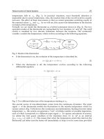
A improvement which can immediately be made is the principle of an (automatic) control
(Fig. 2). Inside the automatic check, the reference variable ω is compared with the
measured output variable of the plant y (control variable), and a suitable output quantity of
the controller u (actuating variable) are calculated inside the control unit of the difference Δy
(control error).
During old time the control unit itself was called the controller, but the modern controllers,
including, between others, the adaptive controllers (Boukhetala et al., 2006), show a
structure where the calculation of the difference between the actual and wished output
value and the calculations of the control algorithm cannot be distinguished in the way just
described. For this reason, the tendency today is towards giving the name controller to the
section in which the variable of release is obtained starting from the reference variable and
the measured control variable.

wi

ω

-

e

Controller

u

+

+

wo
Actuator

Process

+

+

y

Metering Element

Fig. 2. Elements of a control loop
The quantity u is usually given as low-power signal, for example as a digital signal. But with
low power, it is not possible to tack against a physical process. How, for example, could be a
boat to change its course by a rudder angle calculated numerically, which means a sequence
of zeroes and ones at a voltage of 5 V? Because it's not possible directly, a static inverter and
an electric rudder drive are necessary, which may affect the rudder angle and the boat's
route. If the position of the rudder is seen as actuating variable of the system, the static
inverter, the electric rudder drive and the rudder itself from the actuator of the system. The
actuator converts the controller output, a signal of low power, into the actuating variable, a
signal of high power that can directly affect the plant.

Alternatively, the output of the static inverter, that means the armature voltage of the
rudder drive, could be seen as actuating variable. In this case, the actuator would consist
only of static converter, whereas the rudder drive and the rudder should be added to the
plant. These various views already show that a strict separation between the actuator and
the process is not possible. But it is not necessary either, as for the design of the controller;


6

Robust Control, Theory and Applications

we will have to take every transfer characteristic from the controller output to the control
variable into account anyway. Thus, we will treat the actuator as an element of the plant,
and henceforth we will employ the actuating variable to refer to the output quantity of the
controller.
For the feedback of the control variable to the controller the same problem is held, this time
only in the opposite direction: a signal of high power must be transformed into a signal of
low power. This happens in the measuring element, which again shows dynamic properties
that should not be overlooked.
Caused by this feedback, a crucial problem emerges, that we will illustrate by the following
example represented in (Fig. 3). We could formulate strategy of a boat’s automatic control
like this: the larger the deviation from the course is, the more the rudder should be steered
in the opposite direction. At a glance, this strategy seems to be reasonable. If for some
reason a deviation occurs, the rudder is adjusted. By steering into the opposite direction, the
boat receives a rotatory acceleration in the direction of the desired course.
The deviation is reduced until it disappears finally, but the rotating speed does not
disappear with the deviation, it could only be reduced to zero by steering in the other
direction. In this example, because of the rotating speed of the boat will receive a deviation
in the other direction after getting back to the desired course. This is what happened after
the rotating speed will be reduced by counter-steering caused by the new deviation. But as

we already have a new deviation, the whole procedure starts again, only the other way
round. The new deviation could be even greater than the first.
The boat will begin zigzagging its way, if worst comes to worst, with always increasing
deviations. This last case is called instability. If the amplitude of vibration remains the same,
it is called borderline of stability.
Only if the amplitudes decrease the system is stable. To receive an acceptable control
algorithm for the example given, we should have taken the dynamics of the plant into
account when designing the control strategy.
A suitable controller would produce a counter-steering with the rudder right in time to
reduce the rotating speed to zero at the same time the boat gets back on course.

Desired Course
Fig. 3. Automatic cruise control of a boat
This example illustrates the requirements with respect to the controlling devices. A
requirement is accuracy, i.e. the control error should be also small as possible once all the
initial transients are finished and a stationary state is reached. Another requirement is the
speed, i.e. in the case of a changing reference value or a disturbance; the control error should
be eliminated as soon as possible. This is called the response behavior. The requirement of the
third and most important is the stability of the whole system. We will see that these
conditions are contradicted, of this fact of forcing each kind of controller (and therefore
fuzzy controllers, too) to be a compromise between the three.


7

Introduction to Robust Control Techniques

3. Frequency response
If we know a plant’s transfer function, it is easy to construct a suitable controller using this
information. If we cannot develop the transfer function by theoretical considerations, we

could as well employ statistical methods on the basis of a sufficient quantity of values
measured to determine it. This method requires the use of a computer, a plea which was not
available during old time. Consequently, in these days a different method frequently
employed in order to describe a plant's dynamic behavior, frequency response (Franklin et al.,
2002). As we shall see later, the frequency response can easily be measured. Its good
graphical representation leads to a clear method in the design process for simple PID
controllers. Not to mention only several criteria for the stability, which as well are employed
in connection with fuzzy controllers, root in frequency response based characterization of a
plant's behavior.
The easiest way would be to define the frequency response to be the transfer function of a
linear transfer element with purely imaginary values for s.
Consequently, we only have to replace the complex variable s of the transfer function by a
variable purely imaginary. jω : G( jω ) = G(s ) s = jω . The frequency response is thus a complex
function of the parameter ω . Due to the restriction of s to purely imaginary values; the
frequency response is only part of the transfer function, but a part with the special
properties, as the following theorem shows:
Theorem 1 If a linear transfer element has the frequency response G( jω ) , then its response to the
input signal x(t ) = a sin ωt will be-after all initial transients have settled down-the output signal

y(t ) = a G( jω ) sin(ωt + ϕ (G( jω )))

(1)

If the following equation holds:
∞

∫ g(t ) dt ≺ ∞

(2)

0

G( jω ) is obviously the ratio of the output sine amplitude to the input sine amplitude
((transmission) gain or amplification). φ (G( jω ) is the phase of the complex quantity G( jω ) and
shows the delay of the output sine in relation to the input sine (phase lag). g(t ) is the impulse
response of the plant. In case the integral given in (2) does not converge, we have to add the term
r (t ) to the right hand side of (1), which will, even for t → ∞ , not vanish.
The examination of this theorem shows clearly what kind of information about the plant the
frequency response gives: Frequency response characterizes the system's behavior for any
frequency of the input signal. Due to the linearity of the transfer element, the effects caused
by single frequencies of the input signal do not interfere with each other. In this way, we are
now able to predict the resulting effects at the system output for each single signal
component separately, and we can finally superimpose these effects to predict the overall
system output.
Unlike the coefficients of a transfer function, we can measure the amplitude and phase shift
of the frequency response directly: The plant is excited by a sinusoidal input signal of a
certain frequency and amplitude. After all initial transients are installed we obtain a
sinusoidal signal at the output plant, whose phase position and amplitude differ from the
input signal. The quantities can be measured, and depending to (1), this will also instantly


8

Robust Control, Theory and Applications

provide the amplitude and phase lag of the frequency response G( jω ) . In this way, we can
construct a table for different input frequencies that give the principle curve of the
frequency response. Take of measurements for negative values of ω , i.e. for negative
frequencies, which is obviously not possible, but it is not necessary either, delay elements
for the transfer functions rational with real coefficients and for G( jω ) will be conjugate

complex to G( − jω ) . Now, knowing that the function G( jω ) for ω ≥ 0 already contains all
the information needed, we can omit an examination of negative values of ω .

4. Tools for analysis of controls
4.1 Nyquist plot
A Nyquist plot is used in automatic control and signal processing for assessing the stability
of a system with feedback. It is represented by a graph in polar coordinates in which the
gain and phase of a frequency response are plotted. The plot of these phasor quantities
shows the phase as the angle and the magnitude as the distance from the origin (see. Fig.4).
The Nyquist plot is named after Harry Nyquist, a former engineer at Bell Laboratories.
Nyquist Diagram

Nyquist Diagram

50

2.5
0 dB

0 dB

-2 dB

40

2

30

1 4 dB

6 dB
0.5 10 dB

-4 dB

20

-6 dB
-10 dB

Imaginary Axis

Imaginary Axis

1.5 2 dB

0
-0.5

10
2 dB -2 dB
0
-10

-1

-20

-1.5

-30

-2

-40

-2.5
-1

0

1

2

3

4

5

Real Axis

First-order system

-50
-30

-20

-10

0

10

20

30

Real Axis

Second-order systems

Fig. 4. Nyquist plots of linear transfer elements
Assessment of the stability of a closed-loop negative feedback system is done by applying
the Nyquist stability criterion to the Nyquist plot of the open-loop system (i.e. the same
system without its feedback loop). This method is easily applicable even for systems with
delays which may appear difficult to analyze by means of other methods.
Nyquist Criterion: We consider a system whose open loop transfer function (OLTF) is G(s ) ;
when placed in a closed loop with feedback H (s ) , the closed loop transfer function (CLTF)
G
then becomes
. The case where H = 1 is usually taken, when investigating stability,
1 + G.H
and then the characteristic equation, used to predict stability, becomes G + 1 = 0 .
We first construct The Nyquist Contour, a contour that encompasses the right-half of the
complex plane:
•
a path traveling up the jω axis, from 0 -j∞ to 0 + j∞ .

•
a semicircular arc, with radius r → ∞ , that starts at 0 + j∞ and travels clock-wise to
0 -j∞


9

Introduction to Robust Control Techniques

The Nyquist Contour mapped through the function 1 + G(s ) yields a plot of 1 + G(s ) in the
complex plane. By the Argument Principle, the number of clock-wise encirclements of the
origin must be the number of zeros of 1 + G(s ) in the right-half complex plane minus the
poles of 1 + G(s ) in the right-half complex plane. If instead, the contour is mapped through
the open-loop transfer function G(s ) , the result is the Nyquist plot of G(s ) . By counting the
resulting contour's encirclements of −1 , we find the difference between the number of poles
and zeros in the right-half complex plane of 1 + G(s ) . Recalling that the zeros of 1 + G(s ) are
the poles of the closed-loop system, and noting that the poles of 1 + G(s ) are same as the
poles of G(s ) , we now state The Nyquist Criterion:
Given a Nyquist contour Γ s , let P be the number of poles of G(s ) encircled by Γ s and Z be
the number of zeros of 1 + G(s ) encircled by Γ s . Alternatively, and more importantly, Z is
the number of poles of the closed loop system in the right half plane. The resultant contour
in the G(s ) -plane, Γ G( s ) shall encircle (clock-wise) the point ( −1 + j 0 ) N times such
that N = Z − P . For stability of a system, we must have Z = 0 , i.e. the number of closed loop
poles in the right half of the s-plane must be zero. Hence, the number of counterclockwise
encirclements about ( −1 + j 0 ) must be equal to P , the number of open loop poles in the right
half plane (Faulkner, 1969), ( Franklin, 2002).
4.2 Bode diagram
A Bode plot is a plot of either the magnitude or the phase of a transfer function T ( jω ) as a
function of ω . The magnitude plot is the more common plot because it represents the gain
of the system. Therefore, the term “Bode plot” usually refers to the magnitude plot (Thomas,

2004),( William, 1996),( Willy, 2006). The rules for making Bode plots can be derived from
the following transfer function:

⎛ s ⎞
T (s) = K ⎜ ⎟
⎝ ω0 ⎠

±n

where n is a positive integer. For +n as the exponent, the function has n zeros at s = 0 . For
−n , it has n poles at s = 0 . With s = jω , it follows that T ( jω ) = Kj ± n (ω / ω0 )± n ,
T ( jω ) = Kj(ω / ω0 )± n and ∠T ( jω ) = ±n × 90 . If ω is increased by a factor of 10 , T ( jω )
changes by a factor of 10 ± n . Thus a plot of T ( jω ) versus ω on log − log scales has a slope
of log 10 ± n = ± n decades / decade . There are 20dBs in a decade , so the slope can also be
expressed as ±20n dB / decade .
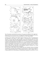
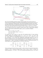
In order to give an example, (Fig. 5) shows the Bode diagrams of the first order and second
order lag. Initial and final values of the phase lag courses can be seen clearly. The same
holds for the initial values of the gain courses. Zero, the final value of these courses, lies at
negative infinity, because of the logarithmic representation. Furthermore, for the second
order lag the resonance magnification for smaller dampings can be see at the resonance
frequency ω0 .
Even with a transfer function being given, a graphical analysis using these two diagrams
might be clearer, and of course it can be tested more easily than, for example, a numerical
analysis done by a computer. It will almost always be easier to estimate the effects of
changes in the values of the parameters of the system, if we use a graphical approach
instead of a numerical one. For this reason, today every control design software tool
provides the possibility of computing the Nyquist plot or the Bode diagram for a given
transfer function by merely clicking on a button.

(

)


10

Robust Control, Theory and Applications
Bode Diagram

Mg i u e( B
an d d )
t

20

0

-20

-40

Pa e( e )
hs dg

-60
0

-45

-90

-2

10

-1

0

10

1

10

2

10
Frequency

3

10

10

4

10

(rad/sec)

First-order systems
Bode Diagram

Mg i u e( B
an d d )
t

100

50

0

-50

Pa e( e )
hs dg

-100
0
-45
-90
-135
-180

-2

10

-1

10

0

10

Frequency

1

10

2

10

3

10

(rad/sec)

Second-order systems
Fig. 5. Bode diagram of first and second-order systems
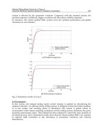
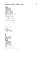
4.3 Evans root locus
In addition to determining the stability of the system, the root locus can be used to design
for the damping ratio and natural frequency of a feedback system (Franklin et al., 2002).
Lines of constant damping ratio can be drawn radially from the origin and lines of constant

natural frequency can be drawn as arcs whose center points coincide with the origin (see.
Fig. 6). By selecting a point along the root locus that coincides with a desired damping ratio
and natural frequency a gain, K, can be calculated and implemented in the controller. More
elaborate techniques of controller design using the root locus are available in most control
textbooks: for instance, lag, lead, PI, PD and PID controllers can be designed approximately
with this technique.
The definition of the damping ratio and natural frequency presumes that the overall
feedback system is well approximated by a second order system, that is, the system has a
dominant pair of poles. This often doesn't happen and so it's good practice to simulate the
final design to check if the project goals are satisfied.


11

Introduction to Robust Control Techniques
Root Locus
20

15

0.105

0.075

0.05

0.032

0.01417.5

0.15

15
12.5
10

10 0.24

7.5
5

Imaginary Axis

5 0.45

2.5

0
2.5

-5 0.45

5
7.5

-10 0.24

10
12.5

-15

15

0.15

-20
-2.5

0.105
-2

0.075

0.05

-1.5

0.032

-1

0.01417.5

-0.5

0

0.5

1

Real Axis

Fig. 6. Evans root locus of a second-order system
Suppose there is a plant (process) with a transfer function expression P(s ) , and a forward
controller with both an adjustable gain K and a transfer function expression C (s ) . A unity
feedback loop is constructed to complete this feedback system. For this system, the overall
transfer function is given by:
T (s ) =

K .C(s ).P(s )
1 + K.C (s ).P(s )

(3)

Thus the closed-loop poles of the transfer function are the solutions to the equation
1 + K .C (s ).P(s ) = 0 . The principal feature of this equation is that roots may be found
wherever K.C .P = −1 . The variability of K , the gain for the controller, removes amplitude
from the equation, meaning the complex valued evaluation of the polynomial in s
C (s ).P(s ) needs to have net phase of 180 deg, wherever there is a closed loop pole. The
geometrical construction adds angle contributions from the vectors extending from each of
the poles of KC to a prospective closed loop root (pole) and subtracts the angle
contributions from similar vectors extending from the zeros, requiring the sum be 180. The
vector formulation arises from the fact that each polynomial term in the factored CP , (s − a)
for example, represents the vector from a which is one of the roots, to s which is the
prospective closed loop pole we are seeking. Thus the entire polynomial is the product of
these terms, and according to vector mathematics the angles add (or subtract, for terms in
the denominator) and lengths multiply (or divide). So to test a point for inclusion on the root
locus, all you do is add the angles to all the open loop poles and zeros. Indeed a form of

protractor, the "spirule" was once used to draw exact root loci.
From the function T (s ) , we can also see that the zeros of the open loop system ( CP ) are also
the zeros of the closed loop system. It is important to note that the root locus only gives the
location of closed loop poles as the gain K is varied, given the open loop transfer function.
The zeros of a system cannot be moved.