Biomedical Engineering 2012 Part 8 potx
Bạn đang xem bản rút gọn của tài liệu. Xem và tải ngay bản đầy đủ của tài liệu tại đây (1.12 MB, 40 trang )
BiomedicalEngineering272
Correlation matrix dimension
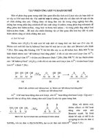
The correlation matrix dimension is carried out to 0.4m (rounded to the nearest integer) for
each side of the autocorrelation curve shown in Fig. 1 below, where –(N-1) ≤ m ≤ N-1; N is
the frame length and m is the distance or lag between data points. The region bounded by
-0.4m and +0.4m contains majority of the statistical information about the signal under
study. Beyond the shaded region the autocorrelation pairs at the positive and corresponding
negative lags diminishes radically, making the calculation unreliable.
-m -0.4m 0 0.4m m
0
Lag
Autocorrelation
Fig. 1. The shaded area containing reliable statistical information for the correlation
(covariance) matrix computation.
Dimension of signal subspace
In general, the dimension (i.e., rank) of the signal subspace is not known a-priori. The proper
dimension of the signal subspace is critical since too low or too high an estimated dimension
yield inaccurate VEP peaks. If the dimension chosen is too low, a highly smoothed spectral
estimate of the VEP waveform is produced, affecting the accuracy of the desired peaks. On
the other hand, too high a dimension introduces a spurious detail in the estimated VEP
waveform, making the discrimination between the desired and unwanted peaks very
difficult. It is crucial to note that as the SNR increases, the separation between the signal
eigenvalues and the noise eigenvalues increases. In other words, for reasonably high SNRs
( 5dB), the signal subspace dimension can be readily obtained by observing the distinctive
gap in the eigenvalue spectrum of the basis matrix covariance. As the SNR reduces, the gap
gets less distinctive and the pertinent signal and noise eigenvalues may be significantly
larger than zero.
As such, the choice of the dimension solely based on the non-zero eigenvalues as devised by
some researchers tends to overestimate the actual dimension of the signal subspace. To
overcome the dimension overestimation, some criteria need to be utilized so that the actual
signal subspace dimension can be estimated more accurately, preventing information loss or
suppressing unwanted details in the recovered signal. There exist many different
approaches for information theoretic criteria for model identification purposes. Two well
known approaches are Akaike information criteria (AIC) by (Akaike, 1973) and minimum
description length (MDL) by (Schwartz, 1978) and (Rissanen, 1978). In this study, the criteria
to be adapted is the AIC approach which has been extended by (Wax & Kailath, 1985) to
handle the signal and noise subspace separation problem from the N snapshots of the
corrupted signals. For our purpose, we consider only one snapshot (N = 1) of the
contaminated signal at one particular time. Assuming that the eigenvalues of the observed
signal (from one snapshot) are denoted as
1
2
p
, we obtain the following:
)2(2
1
ln2)(
1
1
kPk
λ
λ
kP
kAIC
P
kj
j
kP
P
kj
j
(39)
The desired signal subspace dimension L is determined as the value of k [0, P1] for which
the AIC is minimized.
3.1.2 The implementation of GSA technique
Step 1. Compute the covariance matrix of the brain background colored noise R
n
, using the
pre-stimulation EEG sample.
Step 2. Compute the noisy VEP covariance matrix R
y
, using the post-stimulation EEG
sample.
Step 3. Estimate the covariance matrix of the noiseless VEP sample as R
x
= R
y
– R
n
.
Step 4. Perform the generalized eigendecomposition on R
x
and R
n
to satisfy Eq. (34) and
obtain the eigenvector matrix V and the eigenvalue matrix D.
Step 5. Estimate the dimension L of the signal subspace using Eq. (39).
Step 6. Form a diagonal matrix D
L
, from the largest L diagonal values of D.
Step 7. Form a matrix V
L
by retaining only the eigenvectors of V that correspond to the
largest L eigenvalues.
Step 8. Choose a proper value for µ as a compromise between signal distortion and noise
residues. Experimentally, µ = 8 is found to be ideal.
Step 9. Compute the optimal linear estimator as outlined in Eq. (37).
Step 10. Estimate the clean VEP signal using Eq. (38).
SubspaceTechniquesforBrainSignalEnhancement 273
Correlation matrix dimension
The correlation matrix dimension is carried out to 0.4m (rounded to the nearest integer) for
each side of the autocorrelation curve shown in Fig. 1 below, where –(N-1) ≤ m ≤ N-1; N is
the frame length and m is the distance or lag between data points. The region bounded by
-0.4m and +0.4m contains majority of the statistical information about the signal under
study. Beyond the shaded region the autocorrelation pairs at the positive and corresponding
negative lags diminishes radically, making the calculation unreliable.
-m -0.4m 0 0.4m m
0
Lag
Autocorrelation
Fig. 1. The shaded area containing reliable statistical information for the correlation
(covariance) matrix computation.
Dimension of signal subspace
In general, the dimension (i.e., rank) of the signal subspace is not known a-priori. The proper
dimension of the signal subspace is critical since too low or too high an estimated dimension
yield inaccurate VEP peaks. If the dimension chosen is too low, a highly smoothed spectral
estimate of the VEP waveform is produced, affecting the accuracy of the desired peaks. On
the other hand, too high a dimension introduces a spurious detail in the estimated VEP
waveform, making the discrimination between the desired and unwanted peaks very
difficult. It is crucial to note that as the SNR increases, the separation between the signal
eigenvalues and the noise eigenvalues increases. In other words, for reasonably high SNRs
( 5dB), the signal subspace dimension can be readily obtained by observing the distinctive
gap in the eigenvalue spectrum of the basis matrix covariance. As the SNR reduces, the gap
gets less distinctive and the pertinent signal and noise eigenvalues may be significantly
larger than zero.
As such, the choice of the dimension solely based on the non-zero eigenvalues as devised by
some researchers tends to overestimate the actual dimension of the signal subspace. To
overcome the dimension overestimation, some criteria need to be utilized so that the actual
signal subspace dimension can be estimated more accurately, preventing information loss or
suppressing unwanted details in the recovered signal. There exist many different
approaches for information theoretic criteria for model identification purposes. Two well
known approaches are Akaike information criteria (AIC) by (Akaike, 1973) and minimum
description length (MDL) by (Schwartz, 1978) and (Rissanen, 1978). In this study, the criteria
to be adapted is the AIC approach which has been extended by (Wax & Kailath, 1985) to
handle the signal and noise subspace separation problem from the N snapshots of the
corrupted signals. For our purpose, we consider only one snapshot (N = 1) of the
contaminated signal at one particular time. Assuming that the eigenvalues of the observed
signal (from one snapshot) are denoted as
1
2
p
, we obtain the following:
)2(2
1
ln2)(
1
1
kPk
λ
λ
kP
kAIC
P
kj
j
kP
P
kj
j
(39)
The desired signal subspace dimension L is determined as the value of k [0, P1] for which
the AIC is minimized.
3.1.2 The implementation of GSA technique
Step 1. Compute the covariance matrix of the brain background colored noise R
n
, using the
pre-stimulation EEG sample.
Step 2. Compute the noisy VEP covariance matrix R
y
, using the post-stimulation EEG
sample.
Step 3. Estimate the covariance matrix of the noiseless VEP sample as R
x
= R
y
– R
n
.
Step 4. Perform the generalized eigendecomposition on R
x
and R
n
to satisfy Eq. (34) and
obtain the eigenvector matrix V and the eigenvalue matrix D.
Step 5. Estimate the dimension L of the signal subspace using Eq. (39).
Step 6. Form a diagonal matrix D
L
, from the largest L diagonal values of D.
Step 7. Form a matrix V
L
by retaining only the eigenvectors of V that correspond to the
largest L eigenvalues.
Step 8. Choose a proper value for µ as a compromise between signal distortion and noise
residues. Experimentally, µ = 8 is found to be ideal.
Step 9. Compute the optimal linear estimator as outlined in Eq. (37).
Step 10. Estimate the clean VEP signal using Eq. (38).
BiomedicalEngineering274
3.2 Subspace Regularization Method
The subspace regularization method (SRM) (Karjalainen et al., 1999) is combining
regularization and Bayesian approaches for the extraction of EP signals from the measured
data.
In SRM, a model for the EP utilizing a linear combination of some basis vectors as governed
by Eq. (18), is used. Next, the linear observation model of Eq. (18) is further written as
nHθy
(40)
where,
L
represents an L-dimensional parameter vector that needs to be estimated; H
LK x
is defined as the K x L-dimensional basis matrix that does not contain parameters to
be estimated. H is a predetermined pattern based on certain assumptions to be discussed
below. As can be deduced from Eq. (40), the estimated EP signal x
in Eq. (18) is related to H
and
in the following way:
Hθx
(41)
The clean EP signal x in Eq. (41) is modeled as a linear combination of basis vectors
i
Ψ
which make up the columns of the matrix
],, ,[
21 p
ΨΨΨH
. In general, the generic
basis matrix H may comprise equally spaced Gaussian-shaped functions (Karjalainen et al.,
1999) derived from the individual
i
Ψ
, given by the following equation:
K,,,tet
d
i
τt
i
2 1 for )(
2
2
2
)(
Ψ
(42)
where d represents the variance (width) and
i
represents the mean (position) of the function
peak for the given i = 1, 2, , p. Once the parameter H is established and
is estimated, the
single-trial EP can then be determined as follows:
θHx
ˆ
ˆ
(43)
where the hat (
^
) placed over the x and
symbols indicates the “estimate” of the respective
vector.
3.2.1 Regularized least squares solution
The parameter
can be approximated by using a generalized Thikonov regularized least
squares solution stated as:
2
2
2
2
1
)()(min arg
ˆ
*
θθLHθyLθ
θ
(44)
where L
1
and L
2
are the regularization matrices;
is the value of the regularization
parameter;
* is the initial (prior) guess for the solution. The solution in Eq. (44) is in fact the
most commonly used method of regularization of ill-posed problems; Eq. (44) is a
modification of the ordinary weighted least squares solution given as
2
1
)( minarg
ˆ
HθyLθ
θ
LS
(45)
Furthermore, the regularization parameter
in Eq. (44) controls the weight of the side
constraint
2
2
)(
*
θθL
(46)
so that minimization is achieved. Subsequently, Eq. (44) can be simplified further
(Karjalainen et al., 1999) to yield
)() (
ˆ
*
2
2
1
1
2
2
1
θWyWHWHWHθ
TT
(47)
where,
111
LLW
T
and
222
LLW
T
are positive definite weighting matrices.
3.2.2 Bayesian estimation
The regularization process has a close relationship with the Bayesian approach. In addition
to the current information of the parameter (e.g.
) under study, both methods also include
the previous parameter information in their computation. In Bayesian estimation, both
and n in Eq. (40) are treated as random and uncorrelated with each other. The estimator
θ
ˆ
that minimizes the mean square Bayes cost
2
ˆ
θθB E
MS
(48)
is given by the conditional mean
yθθ |
ˆ
E
(49)
of the posterior distribution
)()()( θθyyθ ppp ||
(50)
Subsequently, a linear mean square estimator, known in Bayesian estimation as the
maximum a posteriori estimator (MAP) is expressed as
)() (
ˆ
11111
θθn
T
θn
T
MS
ηRyRHRHRHθ
(51)
where,
n
R is the covariance matrix of the EEG noise n;
θ
R and
θ
η are the covariance
matrix and the mean of the parameter
, respectively―they represent the initial (prior)
information for the parameters
. Equation (51) minimizes Eq. (48) providing that
the errors n are jointly Gaussian with zero mean.
the parameters
are jointly Gaussian random variables.
The covariance matrix
θ
R
can be assumed to be zero if it is not known. In this case, the
estimator in Eq. (51) reduces to the ordinary minimum Gauss-Markov estimator given as
SubspaceTechniquesforBrainSignalEnhancement 275
3.2 Subspace Regularization Method
The subspace regularization method (SRM) (Karjalainen et al., 1999) is combining
regularization and Bayesian approaches for the extraction of EP signals from the measured
data.
In SRM, a model for the EP utilizing a linear combination of some basis vectors as governed
by Eq. (18), is used. Next, the linear observation model of Eq. (18) is further written as
nHθy
(40)
where,
L
represents an L-dimensional parameter vector that needs to be estimated; H
LK x
is defined as the K x L-dimensional basis matrix that does not contain parameters to
be estimated. H is a predetermined pattern based on certain assumptions to be discussed
below. As can be deduced from Eq. (40), the estimated EP signal x
in Eq. (18) is related to H
and
in the following way:
Hθx
(41)
The clean EP signal x in Eq. (41) is modeled as a linear combination of basis vectors
i
Ψ
which make up the columns of the matrix
],, ,[
21 p
ΨΨΨH
. In general, the generic
basis matrix H may comprise equally spaced Gaussian-shaped functions (Karjalainen et al.,
1999) derived from the individual
i
Ψ
, given by the following equation:
K,,,tet
d
i
τt
i
2 1 for )(
2
2
2
)(
Ψ
(42)
where d represents the variance (width) and
i
represents the mean (position) of the function
peak for the given i = 1, 2, , p. Once the parameter H is established and
is estimated, the
single-trial EP can then be determined as follows:
θHx
ˆ
ˆ
(43)
where the hat (
^
) placed over the x and
symbols indicates the “estimate” of the respective
vector.
3.2.1 Regularized least squares solution
The parameter
can be approximated by using a generalized Thikonov regularized least
squares solution stated as:
2
2
2
2
1
)()(min arg
ˆ
*
θθLHθyLθ
θ
(44)
where L
1
and L
2
are the regularization matrices;
is the value of the regularization
parameter;
* is the initial (prior) guess for the solution. The solution in Eq. (44) is in fact the
most commonly used method of regularization of ill-posed problems; Eq. (44) is a
modification of the ordinary weighted least squares solution given as
2
1
)( minarg
ˆ
HθyLθ
θ
LS
(45)
Furthermore, the regularization parameter
in Eq. (44) controls the weight of the side
constraint
2
2
)(
*
θθL
(46)
so that minimization is achieved. Subsequently, Eq. (44) can be simplified further
(Karjalainen et al., 1999) to yield
)() (
ˆ
*
2
2
1
1
2
2
1
θWyWHWHWHθ
TT
(47)
where,
111
LLW
T
and
222
LLW
T
are positive definite weighting matrices.
3.2.2 Bayesian estimation
The regularization process has a close relationship with the Bayesian approach. In addition
to the current information of the parameter (e.g.
) under study, both methods also include
the previous parameter information in their computation. In Bayesian estimation, both
and n in Eq. (40) are treated as random and uncorrelated with each other. The estimator
θ
ˆ
that minimizes the mean square Bayes cost
2
ˆ
θθB E
MS
(48)
is given by the conditional mean
yθθ |
ˆ
E
(49)
of the posterior distribution
)()()( θθyyθ ppp ||
(50)
Subsequently, a linear mean square estimator, known in Bayesian estimation as the
maximum a posteriori estimator (MAP) is expressed as
)() (
ˆ
11111
θθn
T
θn
T
MS
ηRyRHRHRHθ
(51)
where,
n
R is the covariance matrix of the EEG noise n;
θ
R and
θ
η are the covariance
matrix and the mean of the parameter
, respectively―they represent the initial (prior)
information for the parameters
. Equation (51) minimizes Eq. (48) providing that
the errors n are jointly Gaussian with zero mean.
the parameters
are jointly Gaussian random variables.
The covariance matrix
θ
R
can be assumed to be zero if it is not known. In this case, the
estimator in Eq. (51) reduces to the ordinary minimum Gauss-Markov estimator given as
BiomedicalEngineering276
yRHHRHθ
111
)(
ˆ
n
T
n
T
GM
(52)
Next, the estimator in Eq. (52) is equal to the ordinary least squares estimator if the noise are
independent with equal variances (i.e.,
IR
2
nn
σ ); that is
yHHHθ
TT
LS
1
)(
ˆ
(53)
As a matter of fact, Eq. (53) is the Bayesian interpretation of Eq. (47).
3.2.3 Computation of side constraint regularization matrix
As stated previously, the basis matrix H could be produced by using sampled Gaussian or
sigmoid functions, mimicking EP peaks and valleys. A special case exists if the column
vectors that constitute the basis matrix H are mutually orthonormal (i.e.,
I
H
H
T
). The
least squares solution in Eq. (53) can be simplified as
yHθ
T
LS
ˆ
(54)
For clarity, let J be a new basis matrix that represents mutually orthonormal basis vectors.
Now, the least squares solution in Eq. (54) is modified as
yJθ
T
LS
ˆ
(55)
The regularization matrix L
2
is to be derived from an optimal number of column vectors
making up the basis matrix J. The reduced number of J columns, representing the optimal
set of the J basis vectors, can be determined by computing the covariance of
LS
θ
ˆ
in Eq. (55);
that is,
yq
y
TTT
TTTT
LSLSθ
,,,
E
EE
Λ
JRJJyyJ
yJyJθθR
) diag(
)(
ˆˆ
21
(56)
where
λ
1
through λ
q
represent the diagonal eigenvalues of Λ
y.
Equation (56) reveals that the
correlation matrix R
θ
is related to the observation vector correlation matrix R
y
. Specifically,
R
θ
is equal to the the q x q-dimensional eigenvalue matrix Λ
y
. In other words, R
θ
is the
eigenvalue matrix of R
y
, which is the observation vector correlation matrix. Also, the q x q-
dimensional matrix J is actually the eigenvector matrix of R
y
. Even though there are q
diagonal eigenvalues
,
the reduced basis matrix J, denoted as J
x
, is the q x p dimensional
eigenvectors that are associated with the
p largest (i.e., non-zero) eigenvalues of Λ
y.
It is
further assumed that J
x
contains an orthonormal basis of the subspace P. It is desirable that
the EP
Hθx
is closely within this subspace. The projection of x onto P is denoted as
HθJJ )(
xx
. The distance between x and P is
)( )( |||||||| HθJJIHθJJHθ
T
xx
T
xx
(57)
The value of L
2
should be carefully chosen to minimize the side constraint in Eq. (46) which
reduces to
Lθ
for
0
*
θ
. From the inspection of Eq. (57), it can be stated
that
HJJIL )(
2
T
xx
. It is now assumed that L
2
is idempotent and symmetric such that
HJJIH
HJJIJJIH
HJJIHJJILLW
)(
)()(
)()(
222
T
xx
T
T
xx
TT
xx
T
T
xx
T
T
xx
T
(58)
3.2.4 Combination of regularized solution and Bayesian estimation
A new equation is to be generated based on Eq. (47) and Eq. (51); comparisons between
these two equations reveal the following relationships:
1
1
WR
n
, where
111
LLW
T
.
2
21
WR
θ
, where
222
LLW
T
.
*
θη
θ
.
The weight
111
LLW
T
can be represented by
1
n
R since the covariance of the EEG
noise
n
R can be estimated from the pre-stimulation period, during which the EP signal is
absent. On the contrary, the term
1
θ
R
is represented by its equivalent
222
LLW
T
term
obtained from Eq. (58). The new solution based on Eq. (47) and Eq. (51) can now be written
as
*T
xx
T
n
TT
xx
T
n
T
HθJJIHyRHHJJIHHRHθ )()(
ˆ
21
1
21
(59)
Equation (59) is simplified further by treating the prior value
*
θ as zero:
yRHHHHIHHRHθ
1
1
21
)(
ˆ
n
TT
xx
T
n
T
(60)
Therefore, the estimated VEP signal,
x
ˆ
, from Eq. (43) can be expressed as
yRHHJJIHHRHH
θHx
1
1
21
)(
ˆ
ˆ
n
TT
xx
T
n
T
(61)
3.2.5 Strength of the SRM algorithm
The structure of the algorithm in Eq. (61) resembles that of the Karhunen-Loeve transform,
with H
T
as the KLT matrix and H as the inverse KLT matrix. Equation (61) does have extra
terms (besides H
T
and H) which are used for fine tuning. The inclusion of the R
n
1
term
indicates that a pre-whitening stage is incorporated, and the algorithm is able to deal with
both white and colored noise.
SubspaceTechniquesforBrainSignalEnhancement 277
yRHHRHθ
111
)(
ˆ
n
T
n
T
GM
(52)
Next, the estimator in Eq. (52) is equal to the ordinary least squares estimator if the noise are
independent with equal variances (i.e.,
IR
2
nn
σ ); that is
yHHHθ
TT
LS
1
)(
ˆ
(53)
As a matter of fact, Eq. (53) is the Bayesian interpretation of Eq. (47).
3.2.3 Computation of side constraint regularization matrix
As stated previously, the basis matrix H could be produced by using sampled Gaussian or
sigmoid functions, mimicking EP peaks and valleys. A special case exists if the column
vectors that constitute the basis matrix H are mutually orthonormal (i.e.,
I
H
H
T
). The
least squares solution in Eq. (53) can be simplified as
yHθ
T
LS
ˆ
(54)
For clarity, let J be a new basis matrix that represents mutually orthonormal basis vectors.
Now, the least squares solution in Eq. (54) is modified as
yJθ
T
LS
ˆ
(55)
The regularization matrix L
2
is to be derived from an optimal number of column vectors
making up the basis matrix J. The reduced number of J columns, representing the optimal
set of the J basis vectors, can be determined by computing the covariance of
LS
θ
ˆ
in Eq. (55);
that is,
yq
y
TTT
TTTT
LSLSθ
,,,
E
EE
Λ
JRJJyyJ
yJyJθθR
) diag(
)(
ˆˆ
21
(56)
where
λ
1
through λ
q
represent the diagonal eigenvalues of Λ
y.
Equation (56) reveals that the
correlation matrix R
θ
is related to the observation vector correlation matrix R
y
. Specifically,
R
θ
is equal to the the q x q-dimensional eigenvalue matrix Λ
y
. In other words, R
θ
is the
eigenvalue matrix of R
y
, which is the observation vector correlation matrix. Also, the q x q-
dimensional matrix J is actually the eigenvector matrix of R
y
. Even though there are q
diagonal eigenvalues
,
the reduced basis matrix J, denoted as J
x
, is the q x p dimensional
eigenvectors that are associated with the
p largest (i.e., non-zero) eigenvalues of Λ
y.
It is
further assumed that J
x
contains an orthonormal basis of the subspace P. It is desirable that
the EP
Hθx
is closely within this subspace. The projection of x onto P is denoted as
HθJJ )(
xx
. The distance between x and P is
)( )( |||||||| HθJJIHθJJHθ
T
xx
T
xx
(57)
The value of L
2
should be carefully chosen to minimize the side constraint in Eq. (46) which
reduces to
Lθ
for
0
*
θ
. From the inspection of Eq. (57), it can be stated
that
HJJIL )(
2
T
xx
. It is now assumed that L
2
is idempotent and symmetric such that
HJJIH
HJJIJJIH
HJJIHJJILLW
)(
)()(
)()(
222
T
xx
T
T
xx
TT
xx
T
T
xx
T
T
xx
T
(58)
3.2.4 Combination of regularized solution and Bayesian estimation
A new equation is to be generated based on Eq. (47) and Eq. (51); comparisons between
these two equations reveal the following relationships:
1
1
WR
n
, where
111
LLW
T
.
2
21
WR
θ
, where
222
LLW
T
.
*
θη
θ
.
The weight
111
LLW
T
can be represented by
1
n
R since the covariance of the EEG
noise
n
R can be estimated from the pre-stimulation period, during which the EP signal is
absent. On the contrary, the term
1
θ
R
is represented by its equivalent
222
LLW
T
term
obtained from Eq. (58). The new solution based on Eq. (47) and Eq. (51) can now be written
as
*T
xx
T
n
TT
xx
T
n
T
HθJJIHyRHHJJIHHRHθ )()(
ˆ
21
1
21
(59)
Equation (59) is simplified further by treating the prior value
*
θ as zero:
yRHHHHIHHRHθ
1
1
21
)(
ˆ
n
TT
xx
T
n
T
(60)
Therefore, the estimated VEP signal,
x
ˆ
, from Eq. (43) can be expressed as
yRHHJJIHHRHH
θHx
1
1
21
)(
ˆ
ˆ
n
TT
xx
T
n
T
(61)
3.2.5 Strength of the SRM algorithm
The structure of the algorithm in Eq. (61) resembles that of the Karhunen-Loeve transform,
with H
T
as the KLT matrix and H as the inverse KLT matrix. Equation (61) does have extra
terms (besides H
T
and H) which are used for fine tuning. The inclusion of the R
n
1
term
indicates that a pre-whitening stage is incorporated, and the algorithm is able to deal with
both white and colored noise.
BiomedicalEngineering278
3.2.6 Weaknesses of the SRM algorithm
The basis matrix, which serves as one of the algorithm parameters, needs to be carefully
formed by selecting a generic function (e.g., Gaussian or sigmoid) and setting its amplitudes
and widths to mimic EP characteristics. Simply, the improper selection of such a parameter
with a predetermined shape (i.e., amplitudes and variance) somehow pre-meditates or
influences the final outcome of the output waveform.
3.3 Subspace Dynamical Estimation Method
The subspace dynamical estimation method (SDEM) has been proposed by
(Georgiadis et al., 2007) to extract EPs from the observed signals.
In SDEM, a model for the EP utilizes a linear combination of vectors comprising a brain
activity induced by stimulation and other brain activities independent of the stimulus.
Mathematically, the generic model for a single-trial EP follows Eq. (18) and Eq. (40), as this
work is an extension of that proposed earlier by (Karjalainen et al., 1999).
3.3.1 Bayesian estimation
The SDEM scheme makes use of Eq. (48) through Eq. (53) that lead to Eq. (54). In SDEM, the
regularized least squares solution is not included. Also, the basis matrix H is not produced
by using sampled Gaussian or sigmoid functions; the basis matrix will solely be based on
the observed signal under study. For clarity, let Z be a new basis matrix that represents
mutually orthonormal basis vectors to be determined. Now, the least squares solution in
Eq. (55) is modified as
yZθ
T
LS
ˆ
(62)
Based on Eq. (56), it can be deduced that Z in Eq. (62) is actually the eigenvector matrix of
R
y
. The Z term in Eq. (62) can now be represented by its reduced form Z
x
which is associated
with the
p largest (i.e., non-zero) eigenvalues of Λ
y.
It is also assumed that Z
x
contains an
orthonormal basis of the subspace
P. Equation (62) is therefore written as
yZθ
T
x
ˆ
(63)
Therefore, the estimated VEP signal,
x
ˆ
, from Eq. (43) can be expressed as
yZZx
T
xx
ˆ
(64)
The structure in Eq. (64) is actually the Karhunen Loeve transform (KLT) and inverse
Karhunen Loeve transform (IKLT), since the eigenvectors Z which is derived from the
eigendecomposition of the symmetric matrix R
y
is always unitary. What is achieved in
Eq. (64) is that the corrupted EP signal y is decorrelated by the KLT matrix Z
x
T
. Then, the
transformed signal (matrix) is truncated to a certain dimension to suppress the noise
segments. Next, the modified signal is retransformed back into the original form by the
IKLT matrix Z
x
to obtain the desired signal.
3.3.2 Strength of the SDEM algorithm
The state space model is dependent on a basis matrix to be directly produced by performing
eigendecomposition operation on the correlation matrix of the noisy observation. Contrary
to SRM, SDEM makes no assumption about the nature of the EP.
3.3.3 Weaknesses of the SDEM algorithm
The SDEM algorithm will work well for any signal that is corrupted by white noise since the
eigenvectors of the corrupted signal is assumed to be the eigenvectors of the clean signal
and white noise. When the noise becomes colored, the assumption will no longer hold and
the algorithm becomes less effective.
4. Results and Discussions
The three subspace techniques discussed above are tested and assessed using artificial and
real human data.
The subspace methods under study are applied to estimate visual evoked potentials (VEPs)
which are highly corrupted by spontaneous electroencephalogram (EEG) signals. Thorough
simulations using realistically generated VEPs and EEGs at SNRs ranging from 0 to -10 dB
are performed. Later, the algorithms are assessed in their abilities to detect the latencies of
the P100, P200 and P300 components.
Next, the validity and the effectiveness of the algorithms to detect the P100's (used in
objective assessment of visual pathways) are evaluated using real patient data collected
from a hospital. The efficiencies of the studied techniques are then compared among one
another.
4.1 Results from Simulated Data
In the first part of this section, the performances of the GSA, SRM, and SDEM in estimating
the P100, P200, and P300 are tested using artificially generated VEP signals corrupted with
colored noise at different SNR values.
Artificial VEP and EEG waveforms are generated and added to each other in order to create
a noisy VEP. The clean VEP,
x(k)
M
, is generated by superimposing J Gaussian
functions, each of which having a different amplitude (
A), variance (
2
) and mean (
) as
given by the following equations (Andrews et al., 2005).
T
J
n
n
kk
)()(
1
gx
(65)
where g
n
(k) = [g
n1
, g
n2
, …, g
nM
], for k = 1, 2, , M, with the individual g
nk
given as
2
2
2
)(
2
2
n
n
σ
μk
n
n
nk
e
πσ
A
g
(66)
SubspaceTechniquesforBrainSignalEnhancement 279
3.2.6 Weaknesses of the SRM algorithm
The basis matrix, which serves as one of the algorithm parameters, needs to be carefully
formed by selecting a generic function (e.g., Gaussian or sigmoid) and setting its amplitudes
and widths to mimic EP characteristics. Simply, the improper selection of such a parameter
with a predetermined shape (i.e., amplitudes and variance) somehow pre-meditates or
influences the final outcome of the output waveform.
3.3 Subspace Dynamical Estimation Method
The subspace dynamical estimation method (SDEM) has been proposed by
(Georgiadis et al., 2007) to extract EPs from the observed signals.
In SDEM, a model for the EP utilizes a linear combination of vectors comprising a brain
activity induced by stimulation and other brain activities independent of the stimulus.
Mathematically, the generic model for a single-trial EP follows Eq. (18) and Eq. (40), as this
work is an extension of that proposed earlier by (Karjalainen et al., 1999).
3.3.1 Bayesian estimation
The SDEM scheme makes use of Eq. (48) through Eq. (53) that lead to Eq. (54). In SDEM, the
regularized least squares solution is not included. Also, the basis matrix H is not produced
by using sampled Gaussian or sigmoid functions; the basis matrix will solely be based on
the observed signal under study. For clarity, let Z be a new basis matrix that represents
mutually orthonormal basis vectors to be determined. Now, the least squares solution in
Eq. (55) is modified as
yZθ
T
LS
ˆ
(62)
Based on Eq. (56), it can be deduced that Z in Eq. (62) is actually the eigenvector matrix of
R
y
. The Z term in Eq. (62) can now be represented by its reduced form Z
x
which is associated
with the
p largest (i.e., non-zero) eigenvalues of Λ
y.
It is also assumed that Z
x
contains an
orthonormal basis of the subspace
P. Equation (62) is therefore written as
yZθ
T
x
ˆ
(63)
Therefore, the estimated VEP signal,
x
ˆ
, from Eq. (43) can be expressed as
yZZx
T
xx
ˆ
(64)
The structure in Eq. (64) is actually the Karhunen Loeve transform (KLT) and inverse
Karhunen Loeve transform (IKLT), since the eigenvectors Z which is derived from the
eigendecomposition of the symmetric matrix R
y
is always unitary. What is achieved in
Eq. (64) is that the corrupted EP signal y is decorrelated by the KLT matrix Z
x
T
. Then, the
transformed signal (matrix) is truncated to a certain dimension to suppress the noise
segments. Next, the modified signal is retransformed back into the original form by the
IKLT matrix Z
x
to obtain the desired signal.
3.3.2 Strength of the SDEM algorithm
The state space model is dependent on a basis matrix to be directly produced by performing
eigendecomposition operation on the correlation matrix of the noisy observation. Contrary
to SRM, SDEM makes no assumption about the nature of the EP.
3.3.3 Weaknesses of the SDEM algorithm
The SDEM algorithm will work well for any signal that is corrupted by white noise since the
eigenvectors of the corrupted signal is assumed to be the eigenvectors of the clean signal
and white noise. When the noise becomes colored, the assumption will no longer hold and
the algorithm becomes less effective.
4. Results and Discussions
The three subspace techniques discussed above are tested and assessed using artificial and
real human data.
The subspace methods under study are applied to estimate visual evoked potentials (VEPs)
which are highly corrupted by spontaneous electroencephalogram (EEG) signals. Thorough
simulations using realistically generated VEPs and EEGs at SNRs ranging from 0 to -10 dB
are performed. Later, the algorithms are assessed in their abilities to detect the latencies of
the P100, P200 and P300 components.
Next, the validity and the effectiveness of the algorithms to detect the P100's (used in
objective assessment of visual pathways) are evaluated using real patient data collected
from a hospital. The efficiencies of the studied techniques are then compared among one
another.
4.1 Results from Simulated Data
In the first part of this section, the performances of the GSA, SRM, and SDEM in estimating
the P100, P200, and P300 are tested using artificially generated VEP signals corrupted with
colored noise at different SNR values.
Artificial VEP and EEG waveforms are generated and added to each other in order to create
a noisy VEP. The clean VEP,
x(k)
M
, is generated by superimposing J Gaussian
functions, each of which having a different amplitude (
A), variance (
2
) and mean (
) as
given by the following equations (Andrews et al., 2005).
T
J
n
n
kk
)()(
1
gx
(65)
where g
n
(k) = [g
n1
, g
n2
, …, g
nM
], for k = 1, 2, , M, with the individual g
nk
given as
2
2
2
)(
2
2
n
n
σ
μk
n
n
nk
e
πσ
A
g
(66)
BiomedicalEngineering280
The values for A,
and
are experimentally tweaked to create arbitrary amplitudes with
precise peak latencies at 100 ms, 200 ms, and 300 ms simulating the real P100, P200 and P300,
respectively.
The EEG colored noise
e(k) can be characterized by an autoregressive (AR) model
(Yu et al., 1994) given by the following equation.
)()4(0510.0)3(3109.0)2(1587.0)1(5084.1)( kkkkkk weeeee (67)
where
w(k) is the input driving noise of the AR filter and e(k) is the filter output. Since noise
is assumed to be additive, Eq. (65) and Eq. (67) are combined to obtain
)()()( kkk exy
(68)
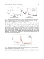
As a preliminary illustration, Fig. 2 below shows, respectively, a sample of artificially
generated VEP, a noisy VEP at SNR = -2 dB, and the extracted VEPs using the GSA, SRM
and SDEM techniques.
0 100 200 300 400
-1
0
1
Time [ms]
(a) VEP and Corrupted VEP
Normalized Amplitude
0 100 200 300 400
-1
0
1
Time [ms]
(b) GSA
Normalized Amplitude
0 100 200 300 400
-1
0
1
Time [ms]
(c) SRM
Normalized Amplitude
0 100 200 300 400
-1
0
1
Time [ms]
(d) SDEM
Normalized Amplitude
Fig. 2. (a) clean VEP (lighter line/color) and corrupted VEP (darker line/color) with
SNR = -2 dB; and the estimated VEPs produced by (b) GSA; (c) SRM; (d) SDEM.
To compare the performances of the algorithms in statistical form, SNR is varied from
0 dB to -13 dB and the algorithms are run 500 times for each value. The average error in
estimating the latencies of P100, P200, and P300 are calculated and tabulated along with the
failure rate in Table 1 below. Any trial is noted as a failure with respect to a certain peak if
the waveform fails to show clearly the pertinent peak.
SNR
[dB]
Peak
Failure rate [%]
Peak
Average error
GSA SRM SDEM GSA SRM SDEM
0
P100 0.6 0.5 1.6 P100 3.7 3.9 4.1
P200 0.4 2.6 3.2 P200 3.9 4.2 4.3
P300 17.8 53.2 40.2 P300 6.5 12.9 9.8
-2
P100 2.2 2.0 2.6 P100 4.1 4.1 4.5
P200 1.4 7.2 9 P200 4.0 5.1 5.3
P300 17.8 55.4 46 P300 6.3 13.3 10.8
-4
P100 3.2 2.8 6.6 P100 4.2 4.2 5.1
P200 5.6 12.2 15.2 P200 4.8 5.8 6.3
P300 21.4 61.4 48.4 P300 6.6 13.8 11.6
-6
P100 5.5 5.7 13.6 P100 4.2 4.5 6.9
P200 4.8 22 22.8 P200 4.5 7.6 8
P300 18.2 60 52.2 P300 6.1 14.0 12.7
-8
P100 8.2 9.8 22.2 P100 4.8 5.7 8.4
P200 8.2 34.8 34.4 P200 4.7 10.0 10.4
P300 17.4 59.6 52.4 P300 6.3 14.5 13
-10
P100 6 16.4 28.8 P100 4.4 7.1 9.6
P200 12.8 37 39.4 P200 5.0 10.6 11.3
P300 18.6 58.4 56.4 P300 6.1 15.2 13.3
Table 1. The failure rate and average errors produced by GSA, SRM and SDEM.
From Table 1, SRM outperforms GSA and SDEM in terms of failure rate for SNRs equal to 0
through -4 dB; however, in terms of average errors, GSA outperforms SRM and SDEM.
From -6 dB and below, GSA is a better estimator compared to both SRM and SDEM.
Overall, it is clear that the proposed GSA algorithm outperforms SRM and SDEM in terms
of accuracy and success rate. All the three algorithms display their best performance in
estimating the latency of the P100 components in comparisons with the other two peaks.
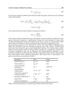
Further, Fig. 3 below illustrates the estimation of VEPs at SNR equal to -10 dB.
SubspaceTechniquesforBrainSignalEnhancement 281
The values for A,
and
are experimentally tweaked to create arbitrary amplitudes with
precise peak latencies at 100 ms, 200 ms, and 300 ms simulating the real P100, P200 and P300,
respectively.
The EEG colored noise
e(k) can be characterized by an autoregressive (AR) model
(Yu et al., 1994) given by the following equation.
)()4(0510.0)3(3109.0)2(1587.0)1(5084.1)( kkkkkk weeeee
(67)
where
w(k) is the input driving noise of the AR filter and e(k) is the filter output. Since noise
is assumed to be additive, Eq. (65) and Eq. (67) are combined to obtain
)()()( kkk exy
(68)
As a preliminary illustration, Fig. 2 below shows, respectively, a sample of artificially
generated VEP, a noisy VEP at SNR = -2 dB, and the extracted VEPs using the GSA, SRM
and SDEM techniques.
0 100 200 300 400
-1
0
1
Time [ms]
(a) VEP and Corrupted VEP
Normalized Amplitude
0 100 200 300 400
-1
0
1
Time [ms]
(b) GSA
Normalized Amplitude
0 100 200 300 400
-1
0
1
Time [ms]
(c) SRM
Normalized Amplitude
0 100 200 300 400
-1
0
1
Time [ms]
(d) SDEM
Normalized Amplitude
Fig. 2. (a) clean VEP (lighter line/color) and corrupted VEP (darker line/color) with
SNR = -2 dB; and the estimated VEPs produced by (b) GSA; (c) SRM; (d) SDEM.
To compare the performances of the algorithms in statistical form, SNR is varied from
0 dB to -13 dB and the algorithms are run 500 times for each value. The average error in
estimating the latencies of P100, P200, and P300 are calculated and tabulated along with the
failure rate in Table 1 below. Any trial is noted as a failure with respect to a certain peak if
the waveform fails to show clearly the pertinent peak.
SNR
[dB]
Peak
Failure rate [%]
Peak
Average error
GSA SRM SDEM GSA SRM SDEM
0
P100 0.6 0.5 1.6 P100 3.7 3.9 4.1
P200 0.4 2.6 3.2 P200 3.9 4.2 4.3
P300 17.8 53.2 40.2 P300 6.5 12.9 9.8
-2
P100 2.2 2.0 2.6 P100 4.1 4.1 4.5
P200 1.4 7.2 9 P200 4.0 5.1 5.3
P300 17.8 55.4 46 P300 6.3 13.3 10.8
-4
P100 3.2 2.8 6.6 P100 4.2 4.2 5.1
P200 5.6 12.2 15.2 P200 4.8 5.8 6.3
P300 21.4 61.4 48.4 P300 6.6 13.8 11.6
-6
P100 5.5 5.7 13.6 P100 4.2 4.5 6.9
P200 4.8 22 22.8 P200 4.5 7.6 8
P300 18.2 60 52.2 P300 6.1 14.0 12.7
-8
P100 8.2 9.8 22.2 P100 4.8 5.7 8.4
P200 8.2 34.8 34.4 P200 4.7 10.0 10.4
P300 17.4 59.6 52.4 P300 6.3 14.5 13
-10
P100 6 16.4 28.8 P100 4.4 7.1 9.6
P200 12.8 37 39.4 P200 5.0 10.6 11.3
P300 18.6 58.4 56.4 P300 6.1 15.2 13.3
Table 1. The failure rate and average errors produced by GSA, SRM and SDEM.
From Table 1, SRM outperforms GSA and SDEM in terms of failure rate for SNRs equal to 0
through -4 dB; however, in terms of average errors, GSA outperforms SRM and SDEM.
From -6 dB and below, GSA is a better estimator compared to both SRM and SDEM.
Overall, it is clear that the proposed GSA algorithm outperforms SRM and SDEM in terms
of accuracy and success rate. All the three algorithms display their best performance in
estimating the latency of the P100 components in comparisons with the other two peaks.
Further, Fig. 3 below illustrates the estimation of VEPs at SNR equal to -10 dB.
BiomedicalEngineering282
0 100 200 300 400
-1
0
1
Time [ms]
(a) VEP and Corrupted VEP
Normalized Amplitude
0 100 200 300 400
-1
0
1
Time [ms]
(b) GSA
Normalized Amplitude
0 100 200 300 400
-2
-1
0
1
Time [ms]
(c) SRM
Normalized Amplitude
0 100 200 300 400
-1
0
1
Time [ms]
(d) SDEM
Normalized Amplitude
Fig. 3. (a) clean VEP (lighter line/color) and corrupted VEP (darker line/color) with
SNR = -10dB; and the estimated VEPs produced by (b) GSA; (c) SRM; (d) SDEM.
4.2 Results of Real Patient Data
This section reveals the accuracy of the GSA, SRM and SDEM techniques in estimating
human P100 peaks, which are used by doctors as objective evaluation of the visual pathway
conduction. Experiments were conducted at Selayang Hospital, Kuala Lumpur using
RETIport32 equipment, and carried out on twenty four subjects having
normal (P100
< 115 ms)
and abnormal (P100 > 115 ms) VEP readings. They were asked to watch a pattern
reversal checkerboard pattern (1
o
full field), the stimulus being a checker reversal
(N = 50 stimuli). Scalp recordings were made according to the International 10/20 System,
with one eye closed at any given time. The active electrode was connected to the middle of
the occipital (O1, O2) area while the reference electrode was attached to the middle of the
forehead. Each trial was pre-filtered in the range 0.1 Hz to 70 Hz and sampled at 512 Hz.
In this study, we will show the results for artifact-free trials of these subjects taken from
their right eyes only. Eighty trials for each subject’s right eye were processed by the VEP
machine using ensemble averaging (EA). The averaged values were readily available and
directly obtained from the equipment. Since EA is a multi-trial scheme, it is expected to
produce good estimation of the P100 that can be used as a baseline for comparing the
performance of the GSA, SRM and SDEM estimators. Further, GSA and SRM require
unprocessed data from the machine. Thus, the equipment was configured accordingly to
generate the raw data. The recording for every trial involved capturing the brain activities
for 333 ms before stimulation was applied; this enabled us to capture the colored EEG noise
alone. The next 333 ms was used to record the post-stimulus EEG, comprising a mixture of
the VEP and EEG. The same process was repeated for the consecutive trials.
For comparisons with EA, the eighty different waveforms per subject produced by SSM
were also averaged. Again, the strategy here was to look for the highest peak from the
averaged waveform. The purpose of averaging the outcome of the SSM was to establish the
performance of GSA, SRM and SDEM as single-trial estimators; any mean peak produced
by any algorithm will be compared with the EA value. The comparisons shall establish the
degree of accuracy of the estimators' individual single-trial outcome.
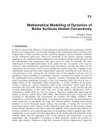
Illustrated in Fig. 4 below is the estimators' extracted Pattern VEPs for S7 from trial #1.
0 108 150
-0.8
-0.6
-0.4
-0.2
0
0.2
0.4
0.6
0.8
1
Time [ms]
Normalized Amplitude
Corrupted VEP
GSA
SRM
SDEM
Fig. 4. The P100 of the seventh subject (S7) taken from trial # 1 (note: the P100 produced by
the EA method is at 108 ms as indicated by the vertical dotted line).
It is to be noted that any peaks that occur below 90 ms are noise and are therefore ignored.
Attention is given to any dominant (i.e., highest) peak(s) from 90 to 150 ms. From Fig. 4, the
corrupted VEP (unprocessed raw signal) contains two dominant peaks at 107 and 115 ms,
with the one at 115 ms being slightly higher. The highest peak produced by GSA is at 108
ms, which is the same as that obtained by EA. The SRM estimator produces two peaks at 107
and 115 ms, with the most dominant peak at 115 ms. The SDEM algorithm shows the
dominant peak at 112 ms. In brief, our GSA technique frequently produces lower mean
errors in detecting the P100 components from the real patient data.
Further, Table 2 below summarizes the mean values of the P100's by EA, GSA, SRM and
SDEM for the twenty four subjects.
SubspaceTechniquesforBrainSignalEnhancement 283
0 100 200 300 400
-1
0
1
Time [ms]
(a) VEP and Corrupted VEP
Normalized Amplitude
0 100 200 300 400
-1
0
1
Time [ms]
(b) GSA
Normalized Amplitude
0 100 200 300 400
-2
-1
0
1
Time [ms]
(c) SRM
Normalized Amplitude
0 100 200 300 400
-1
0
1
Time [ms]
(d) SDEM
Normalized Amplitude
Fig. 3. (a) clean VEP (lighter line/color) and corrupted VEP (darker line/color) with
SNR = -10dB; and the estimated VEPs produced by (b) GSA; (c) SRM; (d) SDEM.
4.2 Results of Real Patient Data
This section reveals the accuracy of the GSA, SRM and SDEM techniques in estimating
human P100 peaks, which are used by doctors as objective evaluation of the visual pathway
conduction. Experiments were conducted at Selayang Hospital, Kuala Lumpur using
RETIport32 equipment, and carried out on twenty four subjects having
normal (P100
< 115 ms)
and abnormal (P100 > 115 ms) VEP readings. They were asked to watch a pattern
reversal checkerboard pattern (1
o
full field), the stimulus being a checker reversal
(N = 50 stimuli). Scalp recordings were made according to the International 10/20 System,
with one eye closed at any given time. The active electrode was connected to the middle of
the occipital (O1, O2) area while the reference electrode was attached to the middle of the
forehead. Each trial was pre-filtered in the range 0.1 Hz to 70 Hz and sampled at 512 Hz.
In this study, we will show the results for artifact-free trials of these subjects taken from
their right eyes only. Eighty trials for each subject’s right eye were processed by the VEP
machine using ensemble averaging (EA). The averaged values were readily available and
directly obtained from the equipment. Since EA is a multi-trial scheme, it is expected to
produce good estimation of the P100 that can be used as a baseline for comparing the
performance of the GSA, SRM and SDEM estimators. Further, GSA and SRM require
unprocessed data from the machine. Thus, the equipment was configured accordingly to
generate the raw data. The recording for every trial involved capturing the brain activities
for 333 ms before stimulation was applied; this enabled us to capture the colored EEG noise
alone. The next 333 ms was used to record the post-stimulus EEG, comprising a mixture of
the VEP and EEG. The same process was repeated for the consecutive trials.
For comparisons with EA, the eighty different waveforms per subject produced by SSM
were also averaged. Again, the strategy here was to look for the highest peak from the
averaged waveform. The purpose of averaging the outcome of the SSM was to establish the
performance of GSA, SRM and SDEM as single-trial estimators; any mean peak produced
by any algorithm will be compared with the EA value. The comparisons shall establish the
degree of accuracy of the estimators' individual single-trial outcome.
Illustrated in Fig. 4 below is the estimators' extracted Pattern VEPs for S7 from trial #1.
0 108 150
-0.8
-0.6
-0.4
-0.2
0
0.2
0.4
0.6
0.8
1
Time [ms]
Normalized Amplitude
Corrupted VEP
GSA
SRM
SDEM
Fig. 4. The P100 of the seventh subject (S7) taken from trial # 1 (note: the P100 produced by
the EA method is at 108 ms as indicated by the vertical dotted line).
It is to be noted that any peaks that occur below 90 ms are noise and are therefore ignored.
Attention is given to any dominant (i.e., highest) peak(s) from 90 to 150 ms. From Fig. 4, the
corrupted VEP (unprocessed raw signal) contains two dominant peaks at 107 and 115 ms,
with the one at 115 ms being slightly higher. The highest peak produced by GSA is at 108
ms, which is the same as that obtained by EA. The SRM estimator produces two peaks at 107
and 115 ms, with the most dominant peak at 115 ms. The SDEM algorithm shows the
dominant peak at 112 ms. In brief, our GSA technique frequently produces lower mean
errors in detecting the P100 components from the real patient data.
Further, Table 2 below summarizes the mean values of the P100's by EA, GSA, SRM and
SDEM for the twenty four subjects.
BiomedicalEngineering284
Subject EA
Latency [ms] Mean Error
GSA SRM SDEM GSA SRM SDEM
S1 99 99 101 138 0 2 39
S2 100 100 101 101 0 1 1
S3 119 119 118 117 0 1 2
S4 128 130 125 96 2 3 32
S5 99 118 98 98 19 1 1
S6 107 104 103 103 3 4 4
S7 108 110 110 91 2 2 17
S8 107 103 105 105 4 2 2
S9 130 144 155 155 14 25 25
S10 117 107 106 105 10 11 12
S11 119 115 123 98 4 4 21
S12 114 113 114 116 1 0 2
S13 102 96 100 117 0 2 20
S14 123 118 118 90 5 5 33
S15 102 96 108 117 6 6 15
S16 108 108 107 106 0 1 2
S17 107 107 107 106 0 0 1
S18 107 108 110 111 1 3 4
S19 110 106 104 104 4 6 6
S20 130 130 121 128 0 9 2
S21 109 102 102 101 7 7 8
S22 130 135 148 138 5 13 8
S23 102 104 133 133 2 31 31
S24 102 102 102 102 0 0 0
Table 2. The mean values of the P100's produced by GSA, SRM and SDEM for twenty four
subjects.
From Table 2, it is quite clear that GSA outperforms the SRM and SDM techniques in
estimating the P100.
5. Conclusion
In this chapter the foundations of the subspace based signal enhancement techniques are
outlined. The relationships between the principal subspace (signal subspace) and the
maximum energy, and between the complementary subspace (noise subspace) and the
minimum energy, are defined. Next, the eigendecomposition of the autocorrelation matrix
of data corrupted by additive noise, and how it is used to enhance SNR by retaining only the
information in the signal subspace eigenvectors, is explained. Since, finding the dimension
of signal subspace is a critical issue to subspace teachings, the Akaike information criteria is
suggested to be used. Three subspace based techniques, GSA, SRM and SDEM, exploiting
the concept of signal and noise subspaces in different ways, in order to effectively enhance
the SNR in EP environments, are explained. The performances of the techniques are
compared using both artificially generated data and real patient data.
In the first experiment, the techniques are used to estimate the latencies of P100, P200, and
P300, under SNR varying from 0 dB to -10 dB. The EPs are artificially generated and
corrupted by colored noise. The results show better performance by the GSA in terms of
both accuracy and failure rate. This is mainly due to the use of the generalized
eigendecomposition for simultaneous diagonalization of signal and noise autocorrelation
matrices.
In the second experiment the performances are compared using real patient data, and
ensemble averaging is used as a baseline. The GSA is showing closer results to the EA, in
comparisons with SRM and SDEM. This makes the single-trial GSA technique perform like
the multi-trial ensemble averaging in VEP extraction, with the added advantages of
recovering the desired peaks of the individual trial, reducing recording time, and relieving
subjects from fatigue.
In summary, subspace techniques are powerful if used properly to extract biomedical
signals such as EPs which are severely corrupted by additive colored or white noise. Finally,
the signal subspace dimension and the Lagrange multiplier are two crucial parameters that
influence the estimators' performances, and thus require further studies.
6. Acknowledgment
The authors would like to thank Universiti Teknologi PETRONAS for funding this research
project. In addition, the authors would like to thank Dr. Tara Mary George and Mr. Mohd
Zawawi Zakaria of the Ophthalmology Department, Selayang Hospital, Kuala Lumpur who
acquired the Pattern Visual Evoked Potentials data at the hospital.
7. References
Akaike, H. (1973). Information Theory and an Extension of the Maximum Likelihood
Principle, Proceedings of the 2nd Int'l. Symp. Inform. Theory, Supp. to Problems of
Control and Inform. Theory, pp. 267-281, 1973.
Andrews, S.; Palaniappan R. & Kamel N. (2005). Extracting Single Trial Visual Evoked
Potentials using Selective Eigen-Rate Principal Components. World Enformatika
Society Transactions on Engineering, Computing and Technology, vol. 7, August 2005.
Cui, J.; Wong, W. & and Mann, S. (2004). Time-Frequency Analysis of Visual Evoked
Potentials by Means of Matching Pursuit with Chirplet Atoms, Proceedings of the
26th Annual International Conference of the IEEE EMBS, San Francisco, CA, USA, pp.
267-270, September 1-5, 2004.
Deprettere, F. (ed.) (1989). SVD and Signal Processing: Algorithms, Applications and
Architectures, North-Holland Publishing Co., 1989.
SubspaceTechniquesforBrainSignalEnhancement 285
Subject EA
Latency [ms] Mean Error
GSA SRM SDEM GSA SRM SDEM
S1 99 99 101 138 0 2 39
S2 100 100 101 101 0 1 1
S3 119 119 118 117 0 1 2
S4 128 130 125 96 2 3 32
S5 99 118 98 98 19 1 1
S6 107 104 103 103 3 4 4
S7 108 110 110 91 2 2 17
S8 107 103 105 105 4 2 2
S9 130 144 155 155 14 25 25
S10 117 107 106 105 10 11 12
S11 119 115 123 98 4 4 21
S12 114 113 114 116 1 0 2
S13 102 96 100 117 0 2 20
S14 123 118 118 90 5 5 33
S15 102 96 108 117 6 6 15
S16 108 108 107 106 0 1 2
S17 107 107 107 106 0 0 1
S18 107 108 110 111 1 3 4
S19 110 106 104 104 4 6 6
S20 130 130 121 128 0 9 2
S21 109 102 102 101 7 7 8
S22 130 135 148 138 5 13 8
S23 102 104 133 133 2 31 31
S24 102 102 102 102 0 0 0
Table 2. The mean values of the P100's produced by GSA, SRM and SDEM for twenty four
subjects.
From Table 2, it is quite clear that GSA outperforms the SRM and SDM techniques in
estimating the P100.
5. Conclusion
In this chapter the foundations of the subspace based signal enhancement techniques are
outlined. The relationships between the principal subspace (signal subspace) and the
maximum energy, and between the complementary subspace (noise subspace) and the
minimum energy, are defined. Next, the eigendecomposition of the autocorrelation matrix
of data corrupted by additive noise, and how it is used to enhance SNR by retaining only the
information in the signal subspace eigenvectors, is explained. Since, finding the dimension
of signal subspace is a critical issue to subspace teachings, the Akaike information criteria is
suggested to be used. Three subspace based techniques, GSA, SRM and SDEM, exploiting
the concept of signal and noise subspaces in different ways, in order to effectively enhance
the SNR in EP environments, are explained. The performances of the techniques are
compared using both artificially generated data and real patient data.
In the first experiment, the techniques are used to estimate the latencies of P100, P200, and
P300, under SNR varying from 0 dB to -10 dB. The EPs are artificially generated and
corrupted by colored noise. The results show better performance by the GSA in terms of
both accuracy and failure rate. This is mainly due to the use of the generalized
eigendecomposition for simultaneous diagonalization of signal and noise autocorrelation
matrices.
In the second experiment the performances are compared using real patient data, and
ensemble averaging is used as a baseline. The GSA is showing closer results to the EA, in
comparisons with SRM and SDEM. This makes the single-trial GSA technique perform like
the multi-trial ensemble averaging in VEP extraction, with the added advantages of
recovering the desired peaks of the individual trial, reducing recording time, and relieving
subjects from fatigue.
In summary, subspace techniques are powerful if used properly to extract biomedical
signals such as EPs which are severely corrupted by additive colored or white noise. Finally,
the signal subspace dimension and the Lagrange multiplier are two crucial parameters that
influence the estimators' performances, and thus require further studies.
6. Acknowledgment
The authors would like to thank Universiti Teknologi PETRONAS for funding this research
project. In addition, the authors would like to thank Dr. Tara Mary George and Mr. Mohd
Zawawi Zakaria of the Ophthalmology Department, Selayang Hospital, Kuala Lumpur who
acquired the Pattern Visual Evoked Potentials data at the hospital.
7. References
Akaike, H. (1973). Information Theory and an Extension of the Maximum Likelihood
Principle, Proceedings of the 2nd Int'l. Symp. Inform. Theory, Supp. to Problems of
Control and Inform. Theory, pp. 267-281, 1973.
Andrews, S.; Palaniappan R. & Kamel N. (2005). Extracting Single Trial Visual Evoked
Potentials using Selective Eigen-Rate Principal Components. World Enformatika
Society Transactions on Engineering, Computing and Technology, vol. 7, August 2005.
Cui, J.; Wong, W. & and Mann, S. (2004). Time-Frequency Analysis of Visual Evoked
Potentials by Means of Matching Pursuit with Chirplet Atoms, Proceedings of the
26th Annual International Conference of the IEEE EMBS, San Francisco, CA, USA, pp.
267-270, September 1-5, 2004.
Deprettere, F. (ed.) (1989). SVD and Signal Processing: Algorithms, Applications and
Architectures, North-Holland Publishing Co., 1989.
BiomedicalEngineering286
Ephraim, Y. & Van Trees, H. L (1995). A Signal Subspace Approach for Speech
Enhancement. IEEE Transaction on Speech and Audio Processing, vol. 3, no. 4, pp. 251-
266, July 1995.
Georgiadis, S.D.; Ranta-aho, P. O.; Tarvainen, M. P. & Karjalainen, P. A (2007). A Subspace
Method for Dynamical Estimation of Evoked Potentials. Computational Intelligence
and Neuroscience, vol. 2007, article ID 61916, pp. 1-11, September 18, 2007.
Gharieb, R. R. & Cichocki, A (2001). Noise Reduction in Brain Evoked Potentials Based on
Third-Order Correlations. IEEE Transactions on Biomedical Engineering, vol. 48, no. 5,
pp. 501-512, May 2001.
Golub, G. H. & Van Loan, C. F. (1989). Matrix Computations, The Johns Hopkins University
Press, 2nd edition, 1989.
Henning, G. & Husar, P. (1995). Statistical Detection of Visually Evoked Potentials. IEEE
Engineering in Medicine and Biology, July/August 1995.
John, E.; Ruchkin, D. & and Villegas, J. (1964). Experimental background: signal analysis and
behavioral correlates of evoked potential configurations in cats. Ann. NY Acad. Sci.,
vol. 112, pp. 362-420, 1964.
Karjalainen, P. A.; Kaipio, J. P.; Koistinen, A. S. & Vauhkonen, M. (1999). Subspace
Regularization Method for the Single-Trial Estimation of Evoked Potentials. IEEE
Transactions on Biomedical Engineering, vol. 46, no. 7, pp. 849-860, July 1999.
Nidal-Kamel & Zuki-Yusoff, M. (2008). A Generalized Subspace Approach for Estimating
Visual Evoked Potentials, Proceedings of the 30th Annual Conference of the IEEE
Engineering in Medicine and Biology Society (IEEE EMBC'08), Vancouver, Canada,
Aug. 20-24, 2008, pp. 5208-5211.
Regan, D. (1989). Human brain electrophysiology: evoked potentials and evoked magnetic fields in
science and medicine, Elsevier, New York: Elsevier.
Rissanen, J. (1978). Modeling by shortest data description. Automatica, vol. 14,
pp. 465-471, 1978.
Schwartz, G. (1978). Estimating the dimension of a model. Ann. Stat., vol. 6,
pp. 461-464, 1978.
Wax, M. & Kailath, T. (1985). Detection of Signals by Information Theoretic Criteria. IEEE
Transactions on Acoustics, Speech, and Signal Processing, vol. ASSP-33, no. 2, pp. 387-
392, April 1985.
Yu, X. H.; He, Z. Y. & and Zhang, Y. S (1994). Time-Varying Adaptive Filters for Evoked
Potential Estimation. IEEE Transactions on Biomedical Engineering, vol. 41, no. 11,
November 1994.
Zuki-Yusoff, M. & Nidal-Kamel (2009). Estimation of Visual Evoked Potentials for
Measurement of Optical Pathway Conduction (accepted for publication), the 17th
European Signal Processing Conference (EUSIPCO 2009), Glasgow, Scotland,
Aug. 24-28, 2009, to be published.
Zuki-Yusoff, M.; Nidal-Kamel & Fadzil-M.Hani, A. (2008). Single-Trial Extraction of Visual
Evoked Potentials from the Brain, Proceedings of the 16th European Signal Processing
Conference (EUSIPCO 2008), Lausanne, Switzerland, Aug. 25-29, 2008.
Zuki-Yusoff, M.; Nidal-Kamel & Fadzil-M.Hani, A. (2007). Estimation of Visual Evoked
Potentials using a Signal Subspace Approach, Proceedings of the International
Conference on Intelligent and Advanced Systems 2007 (ICIAS 2007), Kuala Lumpur,
Malaysia, Nov. 25-28, 2007, pp. 1157-1162.
ClassicationofMentalTasksusingDifferentSpectralEstimationMethods 287
Classication of Mental Tasks using Different Spectral Estimation
Methods
PabloF.Diez,EricLaciar,VicenteMut,EnriqueAvila,AbelTorres
X
Classification of Mental Tasks using Different
Spectral Estimation Methods
Pablo F. Diez
1
, Eric Laciar
1
, Vicente Mut
2
, Enrique Avila
1
, Abel Torres
3
1
Gabinete de Tecnología Médica, Universidad Nacional de San Juan
2
Instituto de Automática, Universidad Nacional de San Juan
3
Departament ESAII, Universitat Politècnica de Catalunya
1,2
Argentina,
3
Spain
1. Introduction
The electroencephalogram (EEG) is the non-invasive recording of the neuronal electrical
activity. The analysis of EEG signals has become, over the last 20 years, a broad field of
research, including many areas such as brain diseases (Parkinson, Alzheimer, etc.), sleep
disorders, anaesthesia monitoring and more recently, in new augmentatives ways of
communication, such as Brain-Computer Interfaces (BCI).
BCI are devices that provide the brain with a new, non-muscular communication channel
(Wolpaw et al., 2002), which can be useful for persons with motor impairments. A wide
variety of methods to extract features from the EEG signals can be used; these include
spectral estimation techniques, wavelet transform, time-frequency representations, and
others. At this moment, the spectral estimation techniques are the most used methods in the
BCI field.
The processing of EEG signals is an important part in the design of a BCI (Wolpaw et al.,
2002). It is commonly divided in the features extraction and the feature translation (Mason &
Birch, 2003). In this work, we will focus in the EEG features extraction using three different
spectral estimation techniques.
In many studies, the researchers use different spectral estimation techniques like Fourier
Transform (Krusienski et al., 2007), Welch periodogram (Millán et al., 2002); (Millán et al.,
2004) or Autoregressive (AR) modeling (Bufalari et al., 2006); (Krusienski et al., 2006);
(Schlögl et al., 1997) in EEG signals. A review of methods for features extraction and features
translation from these signals can be found in a review from the Third BCI meeting
(McFarland et al., 2006). A comparison between the periodogram and the AR model applied
to EEG signals aimed to clinical areas is presented in (Akin & Kiymik, 2000). Finally, an
extended comparison of classification algorithms can be found in (Lotte et al., 2007).
In this chapter, we compare the performance of three different spectral estimation
techniques for the classification of different mental tasks over two EEG databases. These
techniques are the standard periodogram, the Welch periodogram (both based on Fourier
transform) and Burg method (for AR model-based spectral analysis). For each one of these
methods we compute two parameters: the mean power and the root mean square (RMS) in
15
BiomedicalEngineering288
different frequency bands. Both databases used in this work, are composed by a set of EEG
signals acquired on healthy people. One database is related with motor-imagery tasks and
the other one is related with math and imagery tasks.
The classification of the mental tasks was conducted with different classifiers, such as, linear
discriminate analysis, learning vector quantization, neural networks and support vector
machine.
This chapter is organized as follows. In the next section the databases utilized in this work
are explained. The section 3 contains a description of the estimation spectral methods used.
An explanation of the procedure applies to each database is arrived in section 4. The
different classifiers are briefly described in section 5 and the obtained results are shown in
section 6. Finally, in sections 7 and 8 a discussion about results and the conclusions are
presented.
2. EEG Databases
In this work, we have used two different databases, each one with diverse mental tasks.
2.1. Math-Imagine database
This database was collected in a previous work (Diez & Pi Marti, 2006) in the Laboratory of
Digital Electronics, Faculty of Engineering, National University of San Juan (Argentina).
EEG signals from the scalp of six healthy subjects (4 males and 2 females, 28±2 years) were
acquired while they performed three different mental tasks, namely: (a) Relax task: the
subjects close his eyes and try to relax and think in nothing in particular; (b) Math Task: the
subjects make a regressive count from 3 to 3 beginning in 30, i.e. 30, 27, 24, 3, 0. The subjects
were asked to begin the count once again and try to not verbalize; and (c) Imagine task: the
subjects have to imagine an incandescent lamp at the moment that it is turn on.
For each subject, the EEG signals were acquired using six electrodes of Ag/AgCL in
positions F
3
, F
4
, C
3
, C
4
, P
3
and P
4
according to the 10-20 positioning system. With this
electrodes were configured 4 bipolar channels of measurement (ch1: F
3
-C
3
; ch2:F
4
-C
4
; ch3:P
3
-
C
3
; ch4: P
4
-C
4
). Each channel is composed by an instrumentation amplifier with gain 7000
and CMRR greater than 90dB, a bandpass analogical filter set at 0.1-45Hz and an analogical
to digital converter ADC121S101 of 12 bits accuracy with a sampling rate of 150Hz.
0s 1s 2s 3s 4s 5s 6s 7s 8s 9s
Proposed
Mental Task
Start
trial
Performing
Task
F4
C4
P4
F3
C3
P3
Fig. 1. Electrodes position indicated by grey circles (left), on F
3
, F
4
, C
3
, C
4
, P
3
and P
4
according to 10-20 positioning system. The acquisition protocol is presented on the right.
The subjects were trained to keep the maximal concentration while perform the mental
tasks. Each mental task has a duration of 5s (750 samples) with 3s between them. The
subjects were seated comfortably, with dim lighting, in front of a PC monitor. In which,
were presented to subjects the proposed mental tasks (0-2s), the start signal to begin the trial
(3s) and the final of the trial (8s), in according with the protocol illustrated in Figure 1. No
feedback was presented to subjects during the trials. Every session had 15 trials for each
mental task, i.e., 45 trials in total. Two subjects (Subj#1 and Subj#2) performed 3 sessions;
the others performed only 2 sessions, i.e., two subjects had 135 trials and the rest 90 trials.
The EEG of this database were digitally filtered using a Butterworth bi-directional bandpass
filter, order 10, with 6 and 40Hz as lower and upper cut-off frequencies respectively.
2.2. Motor-Imagery database
This database was acquired in the Department of Medical Informatics, Institute for
Biomedical Engineering, University of Technology Graz (Austria) and it is available free on-
line from (BCI-Competition III
web page). It was recorded from a normal subject (female, 25 years) during a feedback
session. The subject sat in a relaxing chair with armrests. The task was to control a feedback
bar by means of (a) imagery left hand and (b) imagery right hand movements. The order of left
and right cues was random. The experiment consists of 140 trials, conducted on the same
day.
Each trial had the first 2s in silence, at t=2s an acoustic stimulus indicates the beginning of
the trial and a “+” was displayed for 1s; then at t=3s, an arrow (left or right) was displayed
as cue. At the same time the subject was asked to move a bar into the direction of the arrow
(Figure 2). Similar acquisition protocols were implemented in several studies (Schlögl et al.,
1997); (Neuper et al., 1999). The recording was made using a G.tec amplifier and Ag/AgCl
electrodes. Three bipolar EEG channels (anterior ‘+’, posterior ‘-‘) were measured over C
3
, C
z
and C
4
. The EEG was sampled with 128 Hz and analogically filtered between 0.5 and 30 Hz.
The feedback was based on AAR parameters of channel over C
3
and C
4
, the AAR
parameters were combined with a discriminate analysis into one output parameter.
Each EEG record of the motor-imagery database was digitally filtered using a Butterworth
filter, order 8, with 6 and 30 Hz as lower and upper cut-off frequencies respectively.
C3 Cz C4
Fig. 2. Electrodes position indicated by grey circles (left), located ±2.5 cm over the crosses.
The crosses indicates the position of C
3
, C
Z
and C
4
according to 10-20 positionin
g
s
y
stem.
The acquisition protocol is presented on the right.
Trigger
beep
Feedback period
with cue
Displayed
cross
0s
1s 2s 3s
4s
5s
6s 7s
8s 9s
ClassicationofMentalTasksusingDifferentSpectralEstimationMethods 289
different frequency bands. Both databases used in this work, are composed by a set of EEG
signals acquired on healthy people. One database is related with motor-imagery tasks and
the other one is related with math and imagery tasks.
The classification of the mental tasks was conducted with different classifiers, such as, linear
discriminate analysis, learning vector quantization, neural networks and support vector
machine.
This chapter is organized as follows. In the next section the databases utilized in this work
are explained. The section 3 contains a description of the estimation spectral methods used.
An explanation of the procedure applies to each database is arrived in section 4. The
different classifiers are briefly described in section 5 and the obtained results are shown in
section 6. Finally, in sections 7 and 8 a discussion about results and the conclusions are
presented.
2. EEG Databases
In this work, we have used two different databases, each one with diverse mental tasks.
2.1. Math-Imagine database
This database was collected in a previous work (Diez & Pi Marti, 2006) in the Laboratory of
Digital Electronics, Faculty of Engineering, National University of San Juan (Argentina).
EEG signals from the scalp of six healthy subjects (4 males and 2 females, 28±2 years) were
acquired while they performed three different mental tasks, namely: (a) Relax task: the
subjects close his eyes and try to relax and think in nothing in particular; (b) Math Task: the
subjects make a regressive count from 3 to 3 beginning in 30, i.e. 30, 27, 24, 3, 0. The subjects
were asked to begin the count once again and try to not verbalize; and (c) Imagine task: the
subjects have to imagine an incandescent lamp at the moment that it is turn on.
For each subject, the EEG signals were acquired using six electrodes of Ag/AgCL in
positions F
3
, F
4
, C
3
, C
4
, P
3
and P
4
according to the 10-20 positioning system. With this
electrodes were configured 4 bipolar channels of measurement (ch1: F
3
-C
3
; ch2:F
4
-C
4
; ch3:P
3
-
C
3
; ch4: P
4
-C
4
). Each channel is composed by an instrumentation amplifier with gain 7000
and CMRR greater than 90dB, a bandpass analogical filter set at 0.1-45Hz and an analogical
to digital converter ADC121S101 of 12 bits accuracy with a sampling rate of 150Hz.
0s 1s 2s 3s 4s 5s 6s 7s 8s 9s
Proposed
Mental Task
Start
trial
Performing
Task
F4
C4
P4
F3
C3
P3
Fig. 1. Electrodes position indicated by grey circles (left), on F
3
, F
4
, C
3
, C
4
, P
3
and P
4
according to 10-20 positioning system. The acquisition protocol is presented on the right.
The subjects were trained to keep the maximal concentration while perform the mental
tasks. Each mental task has a duration of 5s (750 samples) with 3s between them. The
subjects were seated comfortably, with dim lighting, in front of a PC monitor. In which,
were presented to subjects the proposed mental tasks (0-2s), the start signal to begin the trial
(3s) and the final of the trial (8s), in according with the protocol illustrated in Figure 1. No
feedback was presented to subjects during the trials. Every session had 15 trials for each
mental task, i.e., 45 trials in total. Two subjects (Subj#1 and Subj#2) performed 3 sessions;
the others performed only 2 sessions, i.e., two subjects had 135 trials and the rest 90 trials.
The EEG of this database were digitally filtered using a Butterworth bi-directional bandpass
filter, order 10, with 6 and 40Hz as lower and upper cut-off frequencies respectively.
2.2. Motor-Imagery database
This database was acquired in the Department of Medical Informatics, Institute for
Biomedical Engineering, University of Technology Graz (Austria) and it is available free on-
line from (BCI-Competition III
web page). It was recorded from a normal subject (female, 25 years) during a feedback
session. The subject sat in a relaxing chair with armrests. The task was to control a feedback
bar by means of (a) imagery left hand and (b) imagery right hand movements. The order of left
and right cues was random. The experiment consists of 140 trials, conducted on the same
day.
Each trial had the first 2s in silence, at t=2s an acoustic stimulus indicates the beginning of
the trial and a “+” was displayed for 1s; then at t=3s, an arrow (left or right) was displayed
as cue. At the same time the subject was asked to move a bar into the direction of the arrow
(Figure 2). Similar acquisition protocols were implemented in several studies (Schlögl et al.,
1997); (Neuper et al., 1999). The recording was made using a G.tec amplifier and Ag/AgCl
electrodes. Three bipolar EEG channels (anterior ‘+’, posterior ‘-‘) were measured over C
3
, C
z
and C
4
. The EEG was sampled with 128 Hz and analogically filtered between 0.5 and 30 Hz.
The feedback was based on AAR parameters of channel over C
3
and C
4
, the AAR
parameters were combined with a discriminate analysis into one output parameter.
Each EEG record of the motor-imagery database was digitally filtered using a Butterworth
filter, order 8, with 6 and 30 Hz as lower and upper cut-off frequencies respectively.
C3 Cz C4
Fig. 2. Electrodes position indicated by grey circles (left), located ±2.5 cm over the crosses.
The crosses indicates the position of C
3
, C
Z
and C
4
according to 10-20 positionin
g
s
y
stem.
The acquisition protocol is presented on the right.
Trigger
beep
Feedback period
with cue
Displayed
cross
0s
1s 2s 3s
4s
5s
6s 7s
8s 9s
BiomedicalEngineering290
3. Spectral Analysis
EEG signals were processed in order to estimate the signal Power Spectral Density (PSD),
this section explain the different PSD estimation methods regardless the database used. The
three analysed techniques were: (a) standard periodogram, (b) Welch periodogram and
(c) Burg method.
3.1. Standard Periodogram
The periodogram is considered as a non-parametric spectral analysis since no parametric
assumptions about the signal are incorporated.
This technique was introduced at an early stage in the processing of EEG signals and it is
based in the Fourier Transform. Considering that EEG rhythms are essentially oscillatory
signals, its decomposition in terms of sine and cosine, was found useful (Sörnmo & Laguna,
2005). Basically, the Fourier spectral analysis correlates the signal with sines and cosines of
diverse frequencies and produces a set of coefficients that defines the spectral content of the
analyzed signal. The Fourier Transform computed in the discrete field is known as Discrete
Time Fourier Transform (DTFT).
Thus, the periodogram is an estimation of the PSD based on DTFT of the signal x[n] and it is
defined by the following equation:
2
1
2
ˆ
( ) [ ]
s
N
j fnT
s
P
n
T
S f x n e
N
(1)
where S
P
(f) is the periodogram, T
S
is the sampling period, N is the number of samples of the
signal and f is the frequency. Hence, the periodogram is estimated as the squared magnitude
of the N points DTFT of x[n]. The DTFT is easily computed through the Fast Fourier
Transform (FFT) algorithm and, therefore, also the periodogram.
A variation of the periodogram is the windowed periodogram, i.e., we apply a window, in
the process of computing periodogram. Each kind of window has specific characteristics.
There are many types of windows, such as triangular windows (like Bartlett’s), gaussian
windows (like Hanning’s) and others kinds. These windows are used to deal with the
problem of smearing and leakage, due to the presence of main lobe and side lobes. For more
details see (Sörnmo & Laguna, 2005).
In the standard periodogram, no window is used (although no using window is the same as
using a rectangular window).
In Figure 3, it is presented two periodograms (computed with a 1024 points FFT) of EEG
signals from Motor-Imagery database, where an Event Related Desynchronization (ERD) is
observed (Pfurtscheller & Lopes da Silva, 1999). That means, in channel 1 over C
3
(left
figure) the mean power in μ-band (8 to 12 Hz) is higher than the other one in channel 2 over
C
4
(right figure), i.e., in this trial, it is observed easily that subject imagines a left motor task.
3.2. Welch Periodogram
Welch periodogram is a version modified of the periodogram, it can use windowing or not,
but the principal feature of this method is the averaging periodogram. The consequence of
this averaging is the reduction of the variance of the spectrum, at the expense of a reduction
of spectral resolution
The Welch periodogram can be computed performing the following steps:
1. Split the signal in M overlapped segments of D samples length each.
2. Calculates the periodogram for each segment S
P
(f)
(m)
. Each segment had applied a
window.
3. Hence, the Welch periodogram S
W
(f) is calculated as:
( )
1
1
ˆ ˆ
( ) ( )
M
m
W P
m
S f S f
M
(2)
The quantity of segments M could be calculated as:
1
N D
M
L
(3)
where N is the number of samples of the signal and L is the number of samples overlapping
between the segments. In this work, the overlapping was selected in 50% in all cases, which
is the standard value in computation of Welch periodogram.
0 10 20 30 40 50 60
-90
-80
-70
-60
-50
-40
-30
-20
Frequency (Hz)
Power/frequency (dB/Hz)
Power Spectral Density Estimate via Periodogram
0 10 20 30 40 50 60
-90
-80
-70
-60
-50
-40
-30
-20
Power Spectral Density Estimate via Periodogram
Power/frequency (dB/Hz)
Frequency (Hz)
Fig. 3. Standard Periodograms from Motor-Ima
g
er
y
database, trial nº1, between 4 to 6 s;
from (a) channel 1 (over C
3
) and (b) from channel 2 (over C
4
). In this trial the sub
j
ect
imagines a left motor task, then the mean power in μ-band over C
4
is lower than C
3
. Bot
h
periodograms were estimated with a 1024 points FFT. EEG signals were previously filtered
between 6 and 30 Hz.
(a)
(b)
ClassicationofMentalTasksusingDifferentSpectralEstimationMethods 291
3. Spectral Analysis
EEG signals were processed in order to estimate the signal Power Spectral Density (PSD),
this section explain the different PSD estimation methods regardless the database used. The
three analysed techniques were: (a) standard periodogram, (b) Welch periodogram and
(c) Burg method.
3.1. Standard Periodogram
The periodogram is considered as a non-parametric spectral analysis since no parametric
assumptions about the signal are incorporated.
This technique was introduced at an early stage in the processing of EEG signals and it is
based in the Fourier Transform. Considering that EEG rhythms are essentially oscillatory
signals, its decomposition in terms of sine and cosine, was found useful (Sörnmo & Laguna,
2005). Basically, the Fourier spectral analysis correlates the signal with sines and cosines of
diverse frequencies and produces a set of coefficients that defines the spectral content of the
analyzed signal. The Fourier Transform computed in the discrete field is known as Discrete
Time Fourier Transform (DTFT).
Thus, the periodogram is an estimation of the PSD based on DTFT of the signal x[n] and it is
defined by the following equation:
2
1
2
ˆ
( ) [ ]
s
N
j fnT
s
P
n
T
S f x n e
N
(1)
where S
P
(f) is the periodogram, T
S
is the sampling period, N is the number of samples of the
signal and f is the frequency. Hence, the periodogram is estimated as the squared magnitude
of the N points DTFT of x[n]. The DTFT is easily computed through the Fast Fourier
Transform (FFT) algorithm and, therefore, also the periodogram.
A variation of the periodogram is the windowed periodogram, i.e., we apply a window, in
the process of computing periodogram. Each kind of window has specific characteristics.
There are many types of windows, such as triangular windows (like Bartlett’s), gaussian
windows (like Hanning’s) and others kinds. These windows are used to deal with the
problem of smearing and leakage, due to the presence of main lobe and side lobes. For more
details see (Sörnmo & Laguna, 2005).
In the standard periodogram, no window is used (although no using window is the same as
using a rectangular window).
In Figure 3, it is presented two periodograms (computed with a 1024 points FFT) of EEG
signals from Motor-Imagery database, where an Event Related Desynchronization (ERD) is
observed (Pfurtscheller & Lopes da Silva, 1999). That means, in channel 1 over C
3
(left
figure) the mean power in μ-band (8 to 12 Hz) is higher than the other one in channel 2 over
C
4
(right figure), i.e., in this trial, it is observed easily that subject imagines a left motor task.
3.2. Welch Periodogram
Welch periodogram is a version modified of the periodogram, it can use windowing or not,
but the principal feature of this method is the averaging periodogram. The consequence of
this averaging is the reduction of the variance of the spectrum, at the expense of a reduction
of spectral resolution
The Welch periodogram can be computed performing the following steps:
1. Split the signal in M overlapped segments of D samples length each.
2. Calculates the periodogram for each segment S
P
(f)
(m)
. Each segment had applied a
window.
3. Hence, the Welch periodogram S
W
(f) is calculated as:
( )
1
1
ˆ ˆ
( ) ( )
M
m
W P
m
S f S f
M
(2)
The quantity of segments M could be calculated as:
1
N D
M
L
(3)
where N is the number of samples of the signal and L is the number of samples overlapping
between the segments. In this work, the overlapping was selected in 50% in all cases, which
is the standard value in computation of Welch periodogram.
0 10 20 30 40 50 60
-90
-80
-70
-60
-50
-40
-30
-20
Frequency (Hz)
Power/frequency (dB/Hz)
Power Spectral Density Estimate via Periodogram
0 10 20 30 40 50 60
-90
-80
-70
-60
-50
-40
-30
-20
Power Spectral Density Estimate via Periodogram
Power/frequency (dB/Hz)
Frequency (Hz)
Fig. 3. Standard Periodograms from Motor-Ima
g
er
y
database, trial nº1, between 4 to 6 s;
from (a) channel 1 (over C
3
) and (b) from channel 2 (over C
4
). In this trial the subject
imagines a left motor task, then the mean power in μ-band over C
4
is lower than C
3
. Bot
h
periodograms were estimated with a 1024 points FFT. EEG signals were previously filtered
between 6 and 30 Hz.
(a)
(b)
BiomedicalEngineering292
The resolution R depends on the length of segment D according to:
1
S
R
DT
(4)
Hence, high values of D (higher than 75 %, approximately, of the number of samples of the
signal N) obtain a PSD similar to the standard periodogram. On the contrary, with small
values of D the periodogram is smoothed. This fact can be observed in the Figure 4, where
several Welch periodogram are shown, for different Hamming window lengths (16, 32, 64
and 128 points).
0 10 20 30 40 50 60
-80
-70
-60
-50
-40
-30
Frequency (Hz)
Power/frequency (dB/Hz)
Power Spectral Density Estimate via Welch
Window length:
128 points
0 10 20 30 40 50 60
-80
-70
-60
-50
-40
-30
Frequency (Hz)
Power/frequency (dB/Hz)
Power Spectral Density Estimate via Welch
Window length:
64 points
0 10 20 30 40 50 60
-80
-70
-60
-50
-40
-30
Frequency (Hz)
Power/frequency (dB/Hz)
Power Spectral Density Estimate via Welch
Window length:
32 points
0 10 20 30 40 50 60
-80
-70
-60
-50
-40
-30
Frequency (Hz)
Power/frequency (dB/Hz)
Power Spectral Density Estimate via Welch
Window length:
16 points
Fig. 4. Welch periodo
g
ram computed with a 512 points FFT, for different window len
g
th
(128, 64, 32 and 16 points), from Motor-Imagery database, trial nº1, between 4 to 6 s; from
channel 1 (over C
3
). The periodogram is smoothed when decreasing the window len
g
th. A
Hamming window was applied in all cases. The EEG signal was filtered between 6 to 30 Hz.
3.3. Burg method
If consider the EEG like a linear stochastic signal, the EEG can be modelled as an
autoregressive (AR) model, i.e., the estimation of PSD becomes a problem of system
identification.
An AR modelling is, as depicted in Figure 5, based on white noise υ
(n)
feeding a filter H
(z)
,
thus we obtain the signal x
(n)
. The white noise is considered as zero-mean and variance σ
υ
2
.
The filter H
(z)
is expressed as:
( )
1 2
( ) 1 2
1 1
1
z
p
z p
H
A a z a z a z
(5)
where A
(z)
is a polynomial of order p with coefficients a
p
. Those can be estimated through
different methods, such as autocorrelation (Yule-Walker), covariance, modified covariance
and Burg method. In this work, the Burg method was utilized.
Once we are estimated the coefficients a
p
, the PSD is calculated as:
2
2
2
1
( )
1
s
s
P
j fT p
p
p
T
S f
a e
(6)
where σ is the variance of the input signal and P is the order of the AR model.
The Burg method is a technique to estimate the coefficients a
p
of the AR model. This method
joint the minimization of the forward and backward prediction error variances using the
Levinson-Durbin recursion in the minimization process. The prediction error filter is
estimated using a lattice structure; afterwards, the parameters are transformed into direct
form FIR predictor parameters. Thus, the PSD can be calculated using (6). The Burg
description algorithm is beyond of the scope of this work, for mathematical concerns see
(Sörnmo & Laguna, 2005).
3.3.1. Model order
An issue in parametric PSD is choosing the model order, since it influences the shape of
estimated PSD. A low order means a smooth spectrum and, on the other hand, a high order
results in a PSD with spurious peaks. One more pair of roots of polynomial A
(z)
, i.e., increase
the model order in two, force another peak in the estimated spectrum.
There are a few criteria to estimate “the best order” of the model. These criteria penalises the
complexity of the model when increasing the model order. The most known criteria are the
H
(z)
1
A
(z)
υ
(n)
x
(n)
Fig. 5. Autoregressive modeling: Modeled signal x
(n)
obtained through filterin
g
white noise
υ
(n)
with filter H
(
z
)
.
ClassicationofMentalTasksusingDifferentSpectralEstimationMethods 293
The resolution R depends on the length of segment D according to:
1
S
R
DT
(4)
Hence, high values of D (higher than 75 %, approximately, of the number of samples of the
signal N) obtain a PSD similar to the standard periodogram. On the contrary, with small
values of D the periodogram is smoothed. This fact can be observed in the Figure 4, where
several Welch periodogram are shown, for different Hamming window lengths (16, 32, 64
and 128 points).
0 10 20 30 40 50 60
-80
-70
-60
-50
-40
-30
Frequency (Hz)
Power/frequency (dB/Hz)
Power Spectral Density Estimate via Welch
Window length:
128 points
0 10 20 30 40 50 60
-80
-70
-60
-50
-40
-30
Frequency (Hz)
Power/frequency (dB/Hz)
Power Spectral Density Estimate via Welch
Window length:
64 points
0 10 20 30 40 50 60
-80
-70
-60
-50
-40
-30
Frequency (Hz)
Power/frequency (dB/Hz)
Power Spectral Density Estimate via Welch
Window length:
32 points
0 10 20 30 40 50 60
-80
-70
-60
-50
-40
-30
Frequency (Hz)
Power/frequency (dB/Hz)
Power Spectral Density Estimate via Welch
Window length:
16 points
Fig. 4. Welch periodo
g
ram computed with a 512 points FFT, for different window len
g
th
(128, 64, 32 and 16 points), from Motor-Ima
g
er
y
database, trial nº1, between 4 to 6 s; from
channel 1 (over C
3
). The periodogram is smoothed when decreasing the window len
g
th. A
Hamming window was applied in all cases. The EEG signal was filtered between 6 to 30 Hz.
3.3. Burg method
If consider the EEG like a linear stochastic signal, the EEG can be modelled as an
autoregressive (AR) model, i.e., the estimation of PSD becomes a problem of system
identification.
An AR modelling is, as depicted in Figure 5, based on white noise υ
(n)
feeding a filter H
(z)
,
thus we obtain the signal x
(n)
. The white noise is considered as zero-mean and variance σ
υ
2
.
The filter H
(z)
is expressed as:
( )
1 2
( ) 1 2
1 1
1
z
p
z p
H
A a z a z a z
(5)
where A
(z)
is a polynomial of order p with coefficients a
p
. Those can be estimated through
different methods, such as autocorrelation (Yule-Walker), covariance, modified covariance
and Burg method. In this work, the Burg method was utilized.
Once we are estimated the coefficients a
p
, the PSD is calculated as:
2
2
2
1
( )
1
s
s
P
j fT p
p
p
T
S f
a e
(6)
where σ is the variance of the input signal and P is the order of the AR model.
The Burg method is a technique to estimate the coefficients a
p
of the AR model. This method
joint the minimization of the forward and backward prediction error variances using the
Levinson-Durbin recursion in the minimization process. The prediction error filter is
estimated using a lattice structure; afterwards, the parameters are transformed into direct
form FIR predictor parameters. Thus, the PSD can be calculated using (6). The Burg
description algorithm is beyond of the scope of this work, for mathematical concerns see
(Sörnmo & Laguna, 2005).
3.3.1. Model order
An issue in parametric PSD is choosing the model order, since it influences the shape of
estimated PSD. A low order means a smooth spectrum and, on the other hand, a high order
results in a PSD with spurious peaks. One more pair of roots of polynomial A
(z)
, i.e., increase
the model order in two, force another peak in the estimated spectrum.
There are a few criteria to estimate “the best order” of the model. These criteria penalises the
complexity of the model when increasing the model order. The most known criteria are the
H
(z)
1
A
(z)
υ
(n)
x
(n)
Fig. 5. Autoregressive modeling: Modeled signal x
(n)
obtained through filterin
g
white noise
υ
(n)
with filter H
(
z
)
.
BiomedicalEngineering294
Final Prediction Error (FPE), Akaike and modified Akaike (minimum description length of
Rissanen).
For a signal of length N, the penalty function of each criterion is:
2
( )
2
( )
2
( )
ln 2
ln ln
p e
p e
Modif p e
N p
FPE
N p
AIC N p
AIC N
p
N
where σ
e
2
is the prediction error variance.
Figure 6 illustrates the penalty function of the different criteria and it is indicated the best
order found for each method. It was observed, generally, that Akaike and FPE methods
provide the same order of AR model, whereas the modified Akaike criterion does not.
Besides, Akaike and FPE usually overvalue the order of AR model, therefore, it would be
preferable to use the modified Akaike criterion.
In this work, the three criteria were tested, unfortunately, no reliable results were found.
This is, the optimal order varies for each method, also varies for every acquisition channel,
and for data of the same mental task. Hence, the Burg method was analyzed for several
orders on each database, regardless of the order determined by the mentioned criteria.
(7)
(8)
(9)
10 20 30 40 50 60 70 80 90 100
2000
2500
3000
3500
4000
4500
5000
5500
Order
10 20 30 40 50 60 70 80 90 100
3000
3500
4000
4500
5000
Order
10 20 30 40 50 60 70 80 90 100
6000
6100
6200
6300
6400
Order
10 20 30 40 50 60 70 80 90 100
6100
6150
6200
6250
6300
6350
6400
6450
Order
n=47
n=47 n=12
Akaike Criterion
Modified
Akaike Criterion
FPE Criterion
Prediction error
variance:
2
e
Fig. 6. Penalty functions of the different criteria (σ
e
2
, FPE, Akaike and Modified Akaike),
analyzed on Math-Imagery database, channel 2 in first trial.
4. Features Extraction
Although, the three proposed PSD estimation methods were apply on both databases,
special concerns need to be considered for each database. In this section, it is presented an
explanation on the way that each PSD method was applied on each database.
4.1. Features extraction on Math-Imagery database
As was explained in section 2, the signals of this database were filtered between 6 and 40
Hz. The range of frequencies utilized includes the bands α (8 to12Hz), β (12 to 27 Hz), γ
(> 27 Hz) and a part of θ-band (6 to 8Hz). The γ-band is utilized due to the improvement
results shown in (Palaniappan, 2006).
For this database, we proposed a little different division of the EEG bands. The
periodograms were split in bands and sub-bands according to Table I. Due to the shape of
0 10 20 30 40 50 60
-70
-65
-60
-55
-50
-45
-40
-35
-30
Frequency (Hz)
Power/frequency (dB/Hz)
PSD estimate via Burg. Order : 2
0 10 20 30 40 50 60
-80
-70
-60
-50
-40
-30
Frequency (Hz)
Power/frequency (dB/Hz)
PSD estimate via Burg. Order : 4
0 10 20 30 40 50 60
-120
-110
-100
-90
-80
-70
-60
-50
-40
-30
Frequency (Hz)
Power/frequency (dB/Hz)
PSD estimate via Burg. Order : 8
0 10 20 30 40 50 60
-160
-140
-120
-100
-80
-60
-40
Frequency (Hz)
Power/frequency (dB/Hz)
PSD estimate via Burg. Order : 20
Fig. 7. PSD estimated under Burg method for different order of AR model (2, 4 8 and 20).
The spectrum has more peaks when increase the order, according to nº of peaks= AR model
order/2.
ClassicationofMentalTasksusingDifferentSpectralEstimationMethods 295
Final Prediction Error (FPE), Akaike and modified Akaike (minimum description length of
Rissanen).
For a signal of length N, the penalty function of each criterion is:
2
( )
2
( )
2
( )
ln 2
ln ln
p e
p e
Modif p e
N p
FPE
N p
AIC N p
AIC N
p
N
where σ
e
2
is the prediction error variance.
Figure 6 illustrates the penalty function of the different criteria and it is indicated the best
order found for each method. It was observed, generally, that Akaike and FPE methods
provide the same order of AR model, whereas the modified Akaike criterion does not.
Besides, Akaike and FPE usually overvalue the order of AR model, therefore, it would be
preferable to use the modified Akaike criterion.
In this work, the three criteria were tested, unfortunately, no reliable results were found.
This is, the optimal order varies for each method, also varies for every acquisition channel,
and for data of the same mental task. Hence, the Burg method was analyzed for several
orders on each database, regardless of the order determined by the mentioned criteria.
(7)
(8)
(9)
10 20 30 40 50 60 70 80 90 100
2000
2500
3000
3500
4000
4500
5000
5500
Order
10 20 30 40 50 60 70 80 90 100
3000
3500
4000
4500
5000
Order
10 20 30 40 50 60 70 80 90 100
6000
6100
6200
6300
6400
Order
10 20 30 40 50 60 70 80 90 100
6100
6150
6200
6250
6300
6350
6400
6450
Order
n=47
n=47 n=12
Akaike Criterion
Modified
Akaike Criterion
FPE Criterion
Prediction error
variance:
2
e
Fig. 6. Penalty functions of the different criteria (σ
e
2
, FPE, Akaike and Modified Akaike),
analyzed on Math-Imagery database, channel 2 in first trial.
4. Features Extraction
Although, the three proposed PSD estimation methods were apply on both databases,
special concerns need to be considered for each database. In this section, it is presented an
explanation on the way that each PSD method was applied on each database.
4.1. Features extraction on Math-Imagery database
As was explained in section 2, the signals of this database were filtered between 6 and 40
Hz. The range of frequencies utilized includes the bands α (8 to12Hz), β (12 to 27 Hz), γ
(> 27 Hz) and a part of θ-band (6 to 8Hz). The γ-band is utilized due to the improvement
results shown in (Palaniappan, 2006).
For this database, we proposed a little different division of the EEG bands. The
periodograms were split in bands and sub-bands according to Table I. Due to the shape of
0 10 20 30 40 50 60
-70
-65
-60
-55
-50
-45
-40
-35
-30
Frequency (Hz)
Power/frequency (dB/Hz)
PSD estimate via Burg. Order : 2
0 10 20 30 40 50 60
-80
-70
-60
-50
-40
-30
Frequency (Hz)
Power/frequency (dB/Hz)
PSD estimate via Burg. Order : 4
0 10 20 30 40 50 60
-120
-110
-100
-90
-80
-70
-60
-50
-40
-30
Frequency (Hz)
Power/frequency (dB/Hz)
PSD estimate via Burg. Order : 8
0 10 20 30 40 50 60
-160
-140
-120
-100
-80
-60
-40
Frequency (Hz)
Power/frequency (dB/Hz)
PSD estimate via Burg. Order : 20
Fig. 7. PSD estimated under Burg method for different order of AR model (2, 4 8 and 20).
The spectrum has more peaks when increase the order, according to nº of peaks= AR model
order/2.