Micro Electronic and Mechanical Systems 2009 Part 15 pot

Neuron Network Applied to Video Encoder

481

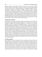
Fig. 3. Basic component of neural network
Dendrites are inputs into neuron. Natural neurons have even hundreds of inputs. Point
where dendrites are touching the neuron is called a synapse. Synapse is characterized by
effectiveness, called synaptic weight. Neuron output is formed in a following way: signals
on dendrites are multiplied by corresponding synaptic weights, results are added and if
they exceed threshold level on the result is applied a transfer function of neuron, which is
marked f on a figure. Only limitation of transfer function is that it must be limited and non-
decreasing. Neuron output is routed to axon, which by its branches transfers result to
dendrites. In this way, output from one layer of network is transferred to the next one.
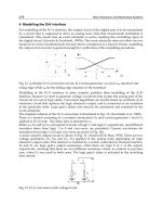
In neural networks, three types of transfer functions are presently being used:
• jumping
• logical with threshold
• sigmoid
All three types are shown in figure 4:


Fig. 4. Three types of transfer functions
The neural network has unique multiprocessing architecture and without much
modification, it surpasses one or even two processors of von Neumann architecture
characterized by serial of sequential information processing (S.P. Teeuwsen at all, 2003). It
has ability to explain every functional dependence and to expose a nature of such
Micro Electronic and Mechanical Systems

482
dependence with no need to external incentives, demands for building a model or its
change. In short, neural network may be considered as a black box capable of predicting
output pattern or a signal after recognizing given input pattern. Once trained, it may

recognize similarities when a new input signal is given, which results in predicted output
signal. There are two categories of neural networks: artificial and biological ones. Artificial
neural networks are in structure, function and in information processing similar to
biological ones. In computer sciences, neural network is an intertwined network of elements
that processes data. One of more important characteristics of neural networks is their
capability to learn from limited set of examples . The neural network is a system comprised
of several simple processors (units, neurons), and every one of them gas its local memory
where it stores processed data. These units are connected by communication channels
(connections). Data exchanged by these channels are usually numerical ones. Units are
processing only their local data and inputs obtained directly through connection.
Limitations of local operators may be removed during training. A large number of neural
networks created as models of biological neural networks. Historically speaking, inspiration
for development of neural networks was in desire to construct an artificial system capable of
refined, maybe even "intelligent" computations in a way similar to that in human brain.
Potentially, neural networks are offering us a possibility to understand functioning of
human brain. Artificial neural networks are a collection of mathematical models that
simulate some of observed capabilities in biological neural systems and has similarities to
adaptable biological learning. They are made of large number of interconnected neurons
(processing elements) which are, similarly to biological neurons, connected by their
connections comprising of permeability (weight) coefficients, whose role is similar to
synapses. Most of neural networks have some kind of rule for "training", which adjusts
coefficients of inter-neural connections based on input data (Cao J, at all 2003). Large
potential of neural networks lays in possibility of parallel data processing, to compute
components independent from each other. Neural networks are systems made of several
simple elements (neurons) that process data parallely.
There are numerous problems in science and engineering that demand extracting useful
information from certain content. For many of those problems, standard techniques as signal
processing, shape recognition, system control, artificial intelligence and so on, are not
adequate. Neural networks are an attempt to solve these problems in a similar way as in
human brain. Like human brain, neural networks are able to learn from given data; later, when

they encounter the same or similar data, they are able to give correct or approximate result.
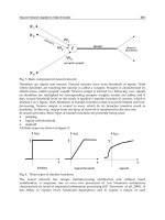
Artificial neuron, based on sum input and transfer function, computes output values. The
following figure shows an artificial neuron:


Fig. 5. Artificial neuron
Neuron Network Applied to Video Encoder

483
The neural network model consists of:
• neural transfer function
• network topology, i.e. a way of interconnecting between neurons,
• learning laws
According to topology, networks are differing by a number of neural layers. Usually each
layer receives inputs from previous one, and sends its outputs to the next layer. The first
neural layer is called input layer, the last one is output layer and other layers are called
hidden layers. Due to a way of interconnecting between neurons, networks may be divided
to recursive and non-recursive ones. In recursive neural networks, higher layers return
information to lower ones, while in non-recursive ones there is a signal flow only from
lower to higher layers.
Neural networks learn from examples. Certainly there must be many examples, often even
tens of thousands. Essence of a learning process is that it causes corrections in synaptic
weights. When new input data cause no more changes in these coefficients, it is considered
that a network is trained to solve a problem. Training may be done in several ways:
controlled training, training by grading and self-organization.
No matter which learning algorithm is used, processes are in essence very similar,
consisting from following steps:
1. A set of input data is presented to a network.
2. Network processes information and remembers result (this is a step forward).
3. The error value is calculated by subtracting obtained result from the expected one.

4. For every node a new synaptic weight is calculated (this is a step back).
5. Synaptic weights are changed, or old ones are left and new ones are remembered.
6. On network inputs, a new set of input data is brought to network inputs and steps 1-5
are repeated. When all examples are processed, synaptic weights values are updated
and if an error is under some expected value the network is considered trained.
We will consider two training modes: controlled training and self-organization training.
The back-propagation algorithm is the most popular algorithm for controlled training. The
basic idea is as follows: random pair of input and output results is chosen. Input set of
signals is sent to the network by bringing one signal at each input neuron. These signals are
propagating further through the network, in hidden layers, and after some time a results
show on output. How has this happened?
For every neuron an input value is calculated, in a way we previously explained; signals are
multiplied by synaptic weights of corresponding dendrites, they are added and a neuron's
transfer function is being applied to obtained value. The signal is propagated further
through the network in a same way, until it reaches output dendrites. Then a transformation
is done once again and output values are obtained. The next step is to compare signals
obtained on output axon branches to expected values for given test example. Error value is
calculated for every output branch. If all errors are equal to zero, there is no need for further
training – network is able to perform expected task. However, in most cases error will be
different from zero. Then a modification of synaptic weights of certain nodes is called for.
Self-organized training is a process where a network finds statistical regularities in a set of
input data and automatically develops different behavior regimes depending on input. For
this type of learning, the Kohonen algorithm is used most often.
The network has only two neural layers: input and output one. Output layer is also called a
competitive layer (reason will be explained later). Every input neuron is connected to every
Micro Electronic and Mechanical Systems

484
neuron in output layer. Neurons in output layer are organized in two-dimensional matrix
(Zurada, J. M.1992).

Multilayer neural network with signal propagation forward is one of often used
architectures. Within it, signals are propagating only ahead, and neurons are organized in
layers. Most important properties of multilayer networks with signal propagation forward
are given as following theorems:
1. Multilayer network with a single hidden layer may uniformly approximate any real
continual function on the finite real axis, with arbitrary precision.
2. Multilayer network with two hidden layers may uniformly approximate any real
continual function of several arguments, with arbitrary precision.
Input layer receives data from environment. Hidden layer receives outputs of a previous
layer (in this case, outputs of input layer) and, depending on sum of input weights, gives
output. For more complex problems, sometimes is necessary more than one hidden layer.
Output layer computes, on the basis of weight sum and transfer function, outputs from
neural network.
The following figure shows a neural network with one hidden layer.


Fig. 6. Neural network with one hidden layer and with signal propagation forward
In this work, we used Kohonen neural network, which is a self-organizing map of
properties, belonging to a class of artificial neural networks with unsupervised training
(Kukolj D., Petrov M., 2000). This type of neural network may be observed as topologically
organized neural map with strong associations to some parts of biological central nervous
system. The notion of topological map understands neurons that are spatially organized in
Neuron Network Applied to Video Encoder

485
maps that guard, in a certain way, the topology of input space. Kohonen neural network is
intended for following tasks:
• Quantumization of input space
• Reduction of output space dimension
• Preservation of topology present within structure of input space.

Kohonen neural network is able to classify input samples-vectors, without need to recognize
signals for error. Therefore, it belongs to group of artificial neural networks with
unsupervised learning. In actual use of Kohonen network in algorithm for obstacle
avoidance, network is not trained but enhancement neurons are given values calculated in
advance. Regarding clusterization, if a network may not classify input vector to any output
cluster, than it gives data regarding how much the input vector is similar to every of clusters
defined in advance. Therefore, this paper uses Fuzzy Kohonen neural clusterization network
(FKCN).
Enhancement of h.263 code properties is attained by generating a prototype codebook,
characterized by highly changeable differences in picture blocks. Generating codebook is
attained by training of self-organizing neural network (Haykin, 1994; Lippmann, 1987;
Zurada, 1992). After realization of original training concept (Kukolj and Petrov, 2000), a
single-layer neural network is formed. Every node of output ANN layers represents a
prototype within codebook. Coordinates of every and node within network is represented
by difficulty synaptic coefficients w
i
. After initialization, the code proceeds in two iterative
phases.
First, closest node for every sample is found, using Euclidean distance, and node
coordinates are computed as arithmetic means of coordinates for samples clustered around
every node. The node balancing procedure is continued by confirmation of following
condition:

SKG
K
i
ii
Tww ≤−
∑
=1

'
, (1)
where T
ASE
is equal to a certain part of present value of average square error (ASE).
Variables w
i
and w
i
'
are synaptic vectors of node and in present and previous code iteration.
If above condition is not met, this step is repeating, otherwise the procedure is proceeding
further.
In a second step, so-called dead nodes are considered, i.e. nodes that have no assigned
samples. If there are no dead nodes, T
ASE
has very low positive value. If dead nodes are
existing, value q for pre-defined number of nodes (q<<K), with maximum ASE value, is
found. Then dead node is moved near one randomly chosen node from q nodes with
maximum ASE values. Now new coordinates of the node are as follows:

δ
+=
qnew
i
ww
max
,
Ki , ,1
=

, (2)
where w
max
q
is location of chosen node between q nodes with highest ASE, w
i
new
is new node
location, and δ = [δ
1
, δ
2
, ,δ
n
]
T
are small random numbers. The process of deriving new
coordinates for dead nodes (2) is repeated for all of those nodes. If maximal number of
iteration is achieved, or if in previous and present iteration number of dead nodes is equal to
zero, code ends. Otherwise it returns to first stage.
Micro Electronic and Mechanical Systems

486
4. Application of ANN in video stream coding
The basic way of removing spatial sameness during coding in h.263 code is using of
transformation (DCT) coding (Kukolj at all, 2006). Instead of being transferred in original
shape after DTC coding, data are presented as the coefficient matrix. Advantage of this
transformation is that obtained coefficients could be quantized, which increases the number
of coefficients with zero value. This enables removal of excess bits using entropy coding on
the bit repeating basis (run-length).

This approach is efficient in cases when a block is poor in details, so the energy is localized
in a few first coefficients of DCT transformation. But, when a picture is rich in details, the
energy is equally distributed to other coefficients as well, so after quantization we do not
obtain consecutive zero coefficients. In these cases, coding of those blocks uses much more
bits, since bit-repetition coding could not be efficiently used. Basic way of compression
factor control in this case is increase of quantization step, which brings to loss of small
details in reconstructed block (block is blurred) with highly expressed block-effect on
reconstructed picture (Cloete, Zurada, 2000).
Enclosed improvement of h.263 code is based on detection of these blocks and their
replacement by corresponding ANN node. Basic criterion for critical blocks detection is the
length of generated bits, using the standard h.263 code.
As training set for ANN we used a set of blocks, which are, during the standard h.263
process, represented with more than 10 bits. Boundary level of code length, N=10 bits, have
been chosen with purpose to obtain codebook with 2
N
=1024 prototypes.
In order to obtain training set, video sequences from "Matrix" movie were used, as well as
standard CIF test video sequences "Mobile and calendar" (Hagan , at all 2002). A training set
from about 100,000 samples was obtained for ANN training. As a training result, training set
was transformed into 1024 codebook prototypes with least average square error regarding
the training set.
The modified code is identical with standard way of h.263 compression of video stream
until the stage of move vector compensation. Every block is coded by the standard method
(using DCT transformation and coding on the basis of bit repeating), and than decision on
application of ANN instead of standard approach is made. Two conditions must be fulfilled
in order to use the network.
1. Condition of code length: whether standard approach gives the code longer of 10 bits
as the representation of observed block. This is the primary condition, providing that
ANN is used only in cases when standard code does not give satisfying compression
level.

2. Condition of activation threshold: whether average square error, obtained using
neural network, is within boundaries:

ANM DCT
SKG k SKG≤⋅ (3)
where:
ASE
INN
- average square error obtained using ANN;
ASE
DCT
- average square error obtained using the standard method
k - activation threshold for the network (1.0 - 1.8).
On the basis of these conditions, choice between standard coding method and ANN
application is being made.
Neuron Network Applied to Video Encoder

487

Fig. 7. Changes in h.263 stream format
Format of coded video stream is taken from h.263 syntax (ITU-T, 1996). Data organization in
levels has been kept, as well as a way of representation for block moves vector. A
modification of syntax of block level was done, introducing additional field (1 bit length) in
header of block level (Fig. 3), in order to note which coding method was used in certain
blocks.
5. Results of testing
Testing of the described modified h.263 code was done on dynamic video sequence from the
"Matrix" movie (525 pictures, 640x304 points). Basic measured parameters were the size of
coded video stream and error within coding process. Error is expressed as peak signal to
noise ratio (PSNR):

255 255
10 log
l
PSNR
SKG
⋅
=⋅ (4)
where ASE
l
is average square error of reconstructed picture in comparison to the original
one.
During the testing, quantization step used in standard DCT coding process and activation
threshold of neural network (expressed as coefficient k in formula (4)) were varied as
parameters.
The standard h.263 was used as a reference for comparison of obtained results.
Two series of tests were done. In first group of tests, quantization step has been varied,
while activation threshold was constant (k=1.0). In second group of tests, activation
threshold has been varied, with constant value for quantization step (1.0).
Figure 8 shows the size of obtained coded stream for both methods. It could be seen that
compression level obtained using ANN is higher than one obtained using standard h.263
code. For higher quantum values, comparable sizes of stream are obtained, since in this case
condition of code length for ANN use was not met, so the coding is being done almost
without ANN.
Figure 9. shows the size of error within coded video stream for both methods. It could be
seen that, for same values of used quantum, ANN has insignificantly higher error than the
standard h.263 approach.
Micro Electronic and Mechanical Systems

488

0
200000
400000
600000
800000
1000000
1200000
6 8 10 15 20
quantum
stream size
h.263
h.263+PM


Fig. 8. Dependence of stream size from quantum

29,000
29,200
29,400
29,600
29,800
30,000
30,200
6 8 10 15 20
quantum
PSNR
h.263
h.263+PM

Fig. 9. Dependence of PSNR from quantum
Figures 10. and 11. show results obtained by varying activation threshold of neural network
between 1.0 and 1.8. Due to clearness, results are shown for the first 60 pictures from the test
sequence. Sudden peaks correspond to changes of camera angle (frame).
Neuron Network Applied to Video Encoder

489

0
15000
30000
45000
60000
75000
90000
11 19 27 35 43 51 59
number of a picture
size of coded picture
h.263
ANM
ANM,k=1.2
ANM,k=1.8

Fig. 10. Dependence of compression from the ANN activation threshold

20,000
22,000
24,000
26,000

28,000
30,000
32,000
11 19 27 35 43 51 59
number of a picture
PSNR
h.263
ANM
ANM, k=1.2
ANM, k=1.8


Fig. 11. Dependence of PSNR from the ANN activation threshold
Micro Electronic and Mechanical Systems

490
Obtained results show that with increase of neural network activation threshold,
compression level decreases and quality of video stream increases. Further increase of
activation threshold (above k=1.8), effect of ANN on coding becomes minor.
6. Conclusion
The paper deals with h.263 recommendation for the video stream compression. Basic
purpose of the modification is stream compression enhancement with insignificant losses in
picture quality. Enhancement of the video stream compression is achieved by artificial
neural network. Conditions for its use are described as condition of code length and
condition of activation threshold. These conditions were tested for every block within
picture, so the coding of the block was done by standard approach or by use of neural
network. Results of testing have shown that by this method the higher compression was
achieved with insignificantly higher error in comparison to the standard h.263 code.
7. References
Amer, A. and E. Dubois (2005). “Fast and Reliable structure-oriented Video Noise

compression standards”, Proc. SPIE, Vol. CR60: Standards and Common Interfaces for
estimation”, IEEE Transactions on Circuits and systems for Video technology, Generic
coding of moving pictures and associated audio information: video, Laboratories,
ISSN: 1051-8215 The Netherlands, May 1989, Video Inform. Syst., Philadelphia,
USA, Oct. 1996,
Barsterretxea K, J. M. Tarela, Campo I.D., Digital design of sigmoid approximator for
artifical neural networks, Electronics letters, Vol m38., ISSN:0013-5194 No.1.
January 2002.
Boncelet C. (2005). Handbook of Image and video procesing, 2
th
edit, Elvesier Academic Press.
ISBN 0121197921.
Bourlard, H., T. Adali, S. Bengio, J. Larsen, and S. Douglas, Proceedings of the Twelfth
IEEE Workshop on Neural Networks for Signal Processing, ISSN:0018-9464 IEEE Press,
2002
Bronstein, I. N., K. A. Semeddjajew, G. Mosiol, and H. Muhlig (2005). Taschenbuck der
mathematik, 6
th
edit, ISBN: 978-3-540-72121-5 Verlah Harri Deutch.
Cao J., Wang J., Liao X.F. Novel stability criteria of delayed celluar neural Networks 13 (2),
ISSN: 0022-0000, 2002.
Cloete Ian, Jacek M. Zurada, "Knowledge-Based Neurocomputing", ISBN: 0-262-03274-0The
MIT Press, 2000.
COST211bis/SIM89/37, Description of Reference Model 8 (RM8), PTT Research
Di Ferdinando, R. Calabretta and D. Parisi, “Evolving modular architectures for neural
networks”, in R. French.and J. P. Sougné (eds.) Connectionist models of learning,
development and evolution, pp. 253-262, ISSN:1370-4621 Springer-Verlag: London,
2001.
Faulsett L., Fundamentals of neural networks—architectures, algorithms, and applications
(Englewood Cliffs, NJ: Prentice-Hall, Inc., 1994).

Neuron Network Applied to Video Encoder

491
Fogel, D. B., C.J. Robinson, "Computational Intelligence", ISBN: 0-471-27454-2 John Wiley &
Sons, IEEE Press,
Girod, B., E. Steinbach, and N. Färber, “Comparison of the H.263 and H.261 video
Hagan, H. Demuth, M. Beale, ISBN-10: 0971732108, ISBN-13: 978-0971732100"Neural
Network Design", 2002,
Haykin, S. (1994). Neural Networks, ISSN:1069-2509New York, MacMillan Publ. Co.
Hertz, J., A. Krogh, R. G. Palmer, Introduction to the Theory of Neural Computation, ISBN
0-201-51560-1 Addison-Wesley, 1991.
ITU-T Recommendation (1995): H.262, ISO/IEC 13818-2:1995, Information technology
ITU-T Recommendation (1996): H.223, Video coding for low bit rate communication.
Kukolj, D. and M. Petrov (2000). “Unlabeled data clustering using a heuristic self-
organizing neural network”, ISSN: 1045-9227 IEEE Transactions on Neural Networks,
2000.
Kukolj, Dragan, Branislav Atlagić, Milovan Petrov, Unlabeled data clustering using a re-
organizing neural network, Cybernetics and Systems, An Int. Journal, Vol. 37, No.
7, 2006, pp. 779-790.
LeGall, D.J., “The MPEG video compression algorithm”, ISSN:1110-8657 Signal Processing:
Image Communication, Vol. 4, No. 2, pp. 129-140, April 1992.
Lippmann, R. P. (1987). “An Introduction to Computing with Neural Nets”, ISSN:0164-1212
EEE ASSP Magazine, April 1987, pp. 4-22.
Mandic D., Chambers J., Recurrent Neural Networks for prediction: Learning Algorithms,
Architecture and stability, ISSN:0045-7906 John Wiley & Sons, New York,
2002,
Markoski, B. and Đ. Babić (2007). “Polynominal-based filters in Bandpass Interpolation
and Sampling rate conversion”, ISSN: 1790-5022 WSEAS Transactions on signal
procesing.
Nauck, D. and R. Kruse. Designing Neuro-Fuzzy Systems Through Backpropagation. W.

Pedrycz ed., Fuzzy Modelling: ISSN:01278274 Paradigms and Practice. Kluwer,
Amsterdam, Netherlands 1995.
Nauck, D., C. Borgelt, F. Klawonn, R. Kruse, ISBN:0-89791-658-1 Neuro – Fuzzy – Systeme,
Wiesbaden, 2003.
Nürnberger, A. Radetzky und R. Kruse. A problem specific recurrent neural network for the
description and simulation of dynamic spring models. ISBN 0-7803-4859-1 In Proc.
IEEE International Joint Conference on Neural Networks 1998 (IJCNN '98), 572-576.
Anchorage, Alaska, Mai 1998.
Rijkse, K., “ITU standardisation of very low bitrate video coding algorithms”, ISSN:0923-
5965 Signal Processing: Image Communication, Vol. 7, pp. 553-565, 1995
Roese, J.A., W.K. Pratt, G.S. Robinson, “Interframe cosine transform image coding”, I
SSN:0-
387-08391-X IEEE Trans. Commun., Vol. 25, No. 11, pp. 1329-1339, Nov. 1977.
Schäfer, R., and T. Sikora, “Digital video coding standards and their role in video
communications”, ISSN: 1445-1336Proc. IEEE, Vol. 83, No. 6, pp. 907-924, June 1995.
Teeuwsen, S. P., I. Erlich, & M.A. El-Sharkawi, Neural network based classification method
for small-signal stability assessment, ISSN: 0885-8950 Proc. IEEE Power Technology
Conf.,Bologna, Italy, 2003, 1–6.
Micro Electronic and Mechanical Systems

492
Teeuwsen, S. P., I. Erlich, & M.A. El-Sharkawi, Small-signal stability assessment based on
advanced neural network methods, ISSN: 0885-8950 Proc. IEEE PES Meeting,
Toronto, CA, 2003, 1–8.
Zurada, J. M. (1992). Introduction to Artificial Neural Systems, St. Paul, ISBN:0-13-611435-0.
West Publishing Co.
27
Single Photon Eigen-Problem
with Complex Internal Dynamics
Nenad V. Delić

1
, Jovan P. Šetrajčić
1,8
, Dragoljub Lj. Mirjanić
2,8
,
Zdravko Ivanković
3
, Dobrivoje Martinov
4
, Snežana Jokić
4
,
Ivana Petrevska–Đukić
5
, Dušanka Tešanović
6
and Svetlana Pelemiš
7

1
Department of Physics, Faculty of Sciences, University of Novi Sad,
2
Faculty of Medicine, University of Banja Luka,
3
Faculty of Technical Sciences, University of Novi Sad,
4
Technical Faculty Zrenjanin, University of Novi Sad,
5
UniCredit Bank Srbija, a.d. Novi Sad,

6
Oncology Institute of Vojvodina, Sremska Kamenica,
7
Faculty of Technology Zvornik, University of East Sarajevo,
8
Academy of Sciences and Arts in Banja Luka,
1,3,4,5,6
Vojvodina – Serbia
2,7,8
Republic of Srpska, BiH
1. Introduction
Linearized single photon Hamiltonian is used for the analysis of its features in coordinate
systems of various geometries. As it could have been expected, based on the general theory
of relativity, it turned out that space geometry and physical features are closely interrelated.
In Cartesian’s coordinates single photons are spatial plane waves, while in cylindrical
coordinates they are one-dimensional plane waves the amplitudes of which falls in planes
normal to the direction of propagation. The most general information on single photon
characteristics has been obtained by the analysis in spherical coordinates. The analysis in
this system has shown that single photon spin essentially influences its behavior and that
the wave functions of single photon can be normalized for zero orbital momentum, only.
A free photon Hamiltonian is linearized in the second part of this paper using Pauli’s
matrices. Based on the correspondence of Pauli’s matrices kinematics and the kinematics of
spin operators, it has been proved that a free photon integral of motion is a sum of orbital
momentum and spin momentum for a half one spin. Linearized Hamiltonian represents a
bilinear form of products of spin and momentum operators. Unitary transformation of this
form results in an equivalent Hamiltonian, which has been analyzed by the method of
Green’s functions. The evaluated Green’s function has given possibility for interpretation of
photon reflection as a transformation of photon to anti-photon with energy change equal to
double energy of photon and for spin change equal to Dirac’s constant. Since photon is
relativistic quantum object the exact determining of its characteristics is impossible. It is the

reason for series of experimental works in which photon orbital momentum, which is not
Micro Electronic and Mechanical Systems

494
integral of motion, was investigated. The exposed theory was compared to the mentioned
experiments and in some elements the satisfactory agreement was found.
2. Eigen-problem of single photon Hamiltonian
In the first part of this work the eigen-problem of single photon Hamiltonian was
formulated and solutions were proposed. Based on the general theory of relativity, it turned
out that space geometry and physical features are closely interrelated. Because of that the
analyses was provided in Cartesian’s, cylindrical and spherical coordinate systems.
2.1 Introduction
Classical expression for free photon energy is:

222
zyx
pppcE ++=
, (1.1)
where c is the light velocity in vacuum and p
x
, p
y
and p
z
are the components of photon
momentum. If instead of classical momentum components we use quantum-mechanical
operators p
ν
→
ν

ν
x
ip
∂
∂
−= 
ˆ
; ν = (x,y,z), where
π
≡
2
h

= 1,05456 ⋅ 10
–34
Js is Dirac's constant,
we obtain quantum-mechanical single photon Hamiltonian:

222
ˆˆˆ
ˆ
zyx
pppcH ++±=
. (2.2)
This Hamiltonian is not a linear operator that contradicts the principle of superposition
(Gottifried, 2003; Kadin, 2005). Klein and Gordon (Sapaznjikov, 1983) skirted this problem
solving the eigen-problem of square of Hamiltonian (2.2):

ϕϕ
22

ˆ
EH =
, (2.3)
since the square of Hamiltonian is a linear operator. This approach has given satisfactory
description of single photon behaving. Up to now it is considered that this approach gives
real picture of photon. Here will be demonstrated that Kline–Gordon picture of photon is
incomplete.
Here we shall try to examine single photon behavior by means of linearized Hamiltonian
(2.2). Linearization procedure is analogous to the procedure that was used by Dirac’s in the
analysis of relativistic electron Hamiltonian (Dirac, 1958). We shall take that

(
)
2
222
ˆ
ˆ
ˆ
ˆ
ˆ
ˆ
ˆˆˆ
zyxzyx
pppppp
χβα
++=++
, (2.4)
i.e. we shall transform the sum of squares into the square of the sum using
βα
ˆ

,
ˆ
and
χ
ˆ

matrices. In accordance with (2.4) these matrices fulfill the following relations:

.0
ˆ
ˆˆ
ˆ
ˆˆˆˆˆ
ˆˆ
ˆ
;1
ˆ
ˆ
ˆ
222
=+=+=+
===
βχχβαχχααββα
χβα

(2.5)
It is easy to show (Tošić, et al., 2008; Delić, et al., 2008) that (2.5) conditions are fulfilled by
Pauli’s matrices
Single Photon Eigen-Problem with Complex Internal Dynamics

495

⎟
⎟
⎠
⎞
⎜
⎜
⎝
⎛
−
=
⎟
⎟
⎠
⎞
⎜
⎜
⎝
⎛
−
=
⎟
⎟
⎠
⎞
⎜
⎜
⎝
⎛

=
10
01
ˆ
;
0
0
ˆ
;
01
10
ˆ
χβα
i
i
. (2.6)
Combining (2.6), (2.4) and (2.2), we obtain linearized photon Hamiltonian which completely
reproduces the quantum nature of light (Holbrow, et al., 2001; Torn, et al., 2004) in the form:

⎟
⎟
⎟
⎟
⎠
⎞
⎜
⎜
⎜
⎜
⎝

⎛
∂
∂
−
∂
∂
+
∂
∂
∂
∂
−
∂
∂
∂
∂
±=
⎟
⎟
⎠
⎞
⎜
⎜
⎝
⎛
−+
−
±=
zy
i

x
y
i
xz
i
c
ppip
pipp
cH
zyx
yxz

ˆˆˆ
ˆˆˆ
ˆ
.
(2.7)
Since linearized Hamiltonian is a 2×2 matrix, photon eigen-states must be columns and rows
which two components. Operators of other physical quantities must be represented in the
form of diagonal 2×2 matrices.
At the end of this presentation, it is important to underline the orbital momentum operator
⎟
⎟
⎠
⎞
⎜
⎜
⎝
⎛
L

L
ˆ
0
0
ˆ


;
prL
ˆˆ
ˆ



×=
does not commute with Hamiltonian (2.7). It means that it is not integral of
motion as in Klein-Gordon theory (Davidov, 1963). It can be shown that integral of motion
represents total momentum
⎟
⎟
⎠
⎞
⎜
⎜
⎝
⎛
J
J
ˆ
0

0
ˆ


, where
J
ˆ

is the sum of orbital momentum
L
ˆ

and
rotation momentum
S
ˆ

which corresponds to 1/2 spin.
In further the eigen-problem of linearized single photon Hamiltonian will be analyzed in
Cartesian’s, cylindrical and spherical coordinates.
2.2 Photons in Cartesian's picture
The eigen-problem of single photon Hamiltonian in Cartesian coordinates (we shall take it
with plus sign) has the following form:

⎟
⎟
⎠
⎞
⎜
⎜

⎝
⎛
Ψ
Ψ
=
⎟
⎟
⎠
⎞
⎜
⎜
⎝
⎛
Ψ
Ψ
⎟
⎟
⎟
⎟
⎠
⎞
⎜
⎜
⎜
⎜
⎝
⎛
∂
∂
−

∂
∂
+
∂
∂
∂
∂
−
∂
∂
∂
∂
2
1
2
1
E
zy
i
x
y
i
xz
i
c
, (2.8)
wherefrom we obtain the following system of equations from:

0
21

=Ψ
⎟
⎟
⎠
⎞
⎜
⎜
⎝
⎛
∂
∂
−
∂
∂
+Ψ
⎟
⎠
⎞
⎜
⎝
⎛
−
∂
∂
y
i
x
ik
z
; (2.9a)

0
21
=Ψ
⎟
⎠
⎞
⎜
⎝
⎛
+
∂
∂
−Ψ
⎟
⎟
⎠
⎞
⎜
⎜
⎝
⎛
∂
∂
+
∂
∂
ik
zy
i

x
, (2.9b)
where
c
E
k

=
. It follows from (2.9a) that:

2
1
1
Ψ
⎟
⎟
⎠
⎞
⎜
⎜
⎝
⎛
∂
∂
−
∂
∂
⎟
⎠
⎞

⎜
⎝
⎛
−
∂
∂
=Ψ
−
y
i
x
ik
z
. (2.10)
Micro Electronic and Mechanical Systems

496
Since the operators
ik
z
±
∂
∂
and
y
i
x ∂
∂
±
∂

∂
commute, through (2.10) we come to the following
relation:

0
11
=Ψ
⎟
⎟
⎠
⎞
⎜
⎜
⎝
⎛
∂
∂
+
∂
∂
⎟
⎟
⎠
⎞
⎜
⎜
⎝
⎛
∂
∂

−
∂
∂
+Ψ
⎟
⎠
⎞
⎜
⎝
⎛
−
∂
∂
⎟
⎠
⎞
⎜
⎝
⎛
+
∂
∂
y
i
xy
i
x
ik
z
ik

z
. (2.11)
In the same manner, from (2.9b) and (2.10), we come to the relation:

0
22
=Ψ
⎟
⎟
⎠
⎞
⎜
⎜
⎝
⎛
∂
∂
−
∂
∂
⎟
⎟
⎠
⎞
⎜
⎜
⎝
⎛
∂
∂

+
∂
∂
+Ψ
⎟
⎠
⎞
⎜
⎝
⎛
+
∂
∂
⎟
⎠
⎞
⎜
⎝
⎛
−
∂
∂
y
i
xy
i
x
ik
z
ik

z
. (2.12)
The two last relations are of identical form and can be substituted by one unique relation:

0),,(
2
2
2
2
2
2
2
=Ψ
⎟
⎟
⎠
⎞
⎜
⎜
⎝
⎛
+
∂
∂
+
∂
∂
+
∂
∂

zyxk
zyx
. (2.13)
If we take in (2.13) that
2222
zyx
kkkk ++=
and
)()()(),,( zCyBxAzyx
=
Ψ
, we come to the
following equation:

0
111
2
2
2
2
2
2
2
2
2
=+++++
zyx
k
dz
Cd

C
k
dy
Bd
B
k
dx
Ad
A
, (2.14)
which is fulfilled if:

0;0;0
2
2
2
2
2
2
2
2
2
=+=+=+ Ck
dz
Cd
Bk
dy
Bd
Ak
dx

Ad
zyx
. (2.15)
Equations (2.15) can be easily solved and each of them has two linearly independent
particular integrals:

.e;e
;e;e
;e;e
2211
2211
2211
zz
yy
xx
izkizk
iykiyk
ixkixk
cCcC
bBbB
aAaA
−
−
−
==
==
==

(2.16)
Based on these expressions, we conclude that eigen-vector of single photon

⎟
⎟
⎠
⎞
⎜
⎜
⎝
⎛
Ψ
Ψ
2
1
has the
following form:

⎟
⎟
⎠
⎞
⎜
⎜
⎝
⎛
=
⎟
⎟
⎠
⎞
⎜
⎜

⎝
⎛
Ψ
Ψ
− rki
rki
D
D




e
e
2
1
. (2.17)
Since
k

is a continuous variable, the normalization of (2.17) mast be done to δ–function,
wherefrom follows:

()
)(
e
e
ee
32
kkrdD

rki
rki
rkirki











′
−=
⎟
⎟
⎠
⎞
⎜
⎜
⎝
⎛
∫
−
′′
−
δ
. (2.18)

Single Photon Eigen-Problem with Complex Internal Dynamics

497
Solving these integrals, we come to: 2

D
2
(2π)
3
= 1, wherefrom we get the normalized single
photon eigen-vector as:

⎟
⎟
⎠
⎞
⎜
⎜
⎝
⎛
π
=
⎟
⎟
⎠
⎞
⎜
⎜
⎝
⎛

Ψ
Ψ
−
rki
rki




e
e
4
1
3
2
1
. (2.19)
As it can be seen from (2.19), the components of single photon eigen-vector are progressive
plane wave ~
rki


e
and the regressive one ~
rki


−
e
. Since we consider a free single photon, the

obtained conclusion is physically acceptable.
2.3 Photons in cylindrical picture
In this section of first part of the paper we are going to analyze the same problem in
cylindrical coordinates. Since solving of partial equation of
0)(
2
=Ψ+Δ k
type in cylindrical
coordinates requires more general approach than that which was used in Cartesian's
coordinates, it is necessary to examine single photon eigen-problem in cylindrical system.
In order to examine this problem, we shall start from the equation (2.13) in which Laplacian
Δ≡
∂
∂
+
∂
∂
+
∂
∂
2
2
2
2
2
2
zyx
will be given in cylindrical coordinates (ρ,φ,z) where ρ э [0,∞], φ э [0,2π]
and z э [–∞,+∞]. The Laplacian in cylindrical coordinates has the following form:
2

2
2
2
22
2
11
z∂
∂
+
∂
∂
+
∂
∂
+
∂
∂
=Δ
ϕρ
ρρ
ρ

and therefore (2.13) with Ψ(x,y,z) => Φ(ρ,φ,z), reduces to:

0
11
2
2
2
2

2
22
2
=Φ+
∂
Φ∂
+
∂
Φ∂
+
∂
Φ∂
+
∂
Φ∂
k
z
ϕρ
ρρ
ρ
. (2.20)
The square of wave vector k will be separated into two parts
22222
zzyx
kqkkk +=++
. On the
basis of this the equation (2.20) can be written as follows:

Φ−
∂

Φ∂
−=
∂
Φ∂
+Φ+
∂
Φ∂
+
∂
Φ∂
2
2
2
2
2
2
2
2
2
11
z
k
z
q
ϕρ
ρρ
ρ
. (2.21)
By the substitution:

)(),(),,( zGFz
ϕ
ρ
ϕ
ρ
=
Φ
, (2.22)
the equation (2.21) reduces to:

⎟
⎟
⎠
⎞
⎜
⎜
⎝
⎛
+
∂
−=
⎟
⎟
⎠
⎞
⎜
⎜
⎝
⎛
∂

∂
++
∂
∂
+
∂
∂
Gk
z
Gd
G
F
Fq
FF
F
z
2
2
2
2
2
2
2
2
2
1111
ϕρρρρ
. (2.23)
This equation is fulfilled if:

0
11
2
2
2
2
2
2
=
∂
∂
++
∂
∂
+
∂
∂
ϕρ
ρρ
ρ
F
Fq
FF
; (2.24a)
Micro Electronic and Mechanical Systems

498

0
2

2
2
=+
∂
Gk
z
Gd
z
. (2.24b)
Now we separate the variables by substitution:

)()(),(
ϕ
ρ
ϕ
ρ
SXF
=
, (2.25)
after which, the (2.24a) goes over to:

2
2
2
22
2
2
2
11
m

Sd
S
Xq
XX
X
≡
∂
−=
⎟
⎟
⎠
⎞
⎜
⎜
⎝
⎛
+
∂
∂
+
∂
∂
ϕ
ρ
ρ
ρ
ρ
ρ
. (2.26)
Introduction of the variables separation constant m

2
represents generalization with respect
to approach used in previous section. Since the function S(φ) must be single-sign S(φ) =
S(φ+2π) we must that m is integer, i.e. m = 0,±1, ±2,
Relation (2.26) is separated into two differential equations:

;0
2
2
2
=+ Sm
d
Sd
ϕ

(2.27a)

.0)(
1
2
2
2
2
2
=−++ X
m
q
d
dX
d

Xd
ρρρρ

(2.27b)
The equation (2.24b) has two particular integrals:

zz
izkizk
gGgG
−
== e;e
2211
, (2.28)
while the solution of the equation (2.27a) is:

ϕ
ϕ
im
m
sS e)(
0
=
. (2.29)
By the substitution of argument ρ = b

ξ, the equation (2.27b) reduces to

0
1
2

2
22
2
2
=
⎟
⎟
⎠
⎞
⎜
⎜
⎝
⎛
−++ X
m
bq
d
dX
d
Xd
ξξξξ
, (2.30)
and taking that
q
b
1
=
, we translate (2.30) into Bessel's equation with integer index m:

01

1
2
2
2
2
=
⎟
⎟
⎠
⎞
⎜
⎜
⎝
⎛
−++ X
m
d
dX
d
Xd
ξξξξ
. (2.31)
It means that the solution of (2.27b) is the m–order Bessel’s function: J
m
, i.e.

)()(
0
ρ
ρ

qJaX
m
=
. (2.32)
Taking into account (2.28), (2.29) and (2.32), we obtain the components of single photon
eigen-vector:

ϕϕ
ρϕρρϕρ
im
izk
m
im
izk
m
zz
qJDzqJDz ee)(),,(;ee)(),,(
2211
−
=Φ=Φ
. (2.33a)
Single Photon Eigen-Problem with Complex Internal Dynamics

499
Since q and k
z
are continuous variables, while m is a discrete one the normalization of eigen-
vector must be done partially to δ–functions and partially to Kronecker’s symbol. It means
that normalization condition is the following:
()

)()()()(ee
1
0
)(
)(
2
0
2
2
2
1
qqkkqqJqJddzdDD
zznmmm
zkki
mmi
zzz
′
−
′
−=
′
+
−
∞+∞
∞−
′
−±
′
−±
∫∫∫

δδδρρρρϕ
ϕ
π
.
Using formula for normalization of Bessel functions with integer index (Korn & Korn, 1961):
)(
1
)()(
0
kk
k
kxJxkJxdx
mm
′
−=
′
∫
∞
δ
,
the normalization condition reduces into:
2
2
2
2
1
4
1
π
=+ DD

. It means that normalized single
photon eigen-vector in cylindrical coordinates is given by:

⎟
⎟
⎠
⎞
⎜
⎜
⎝
⎛
=
⎟
⎟
⎠
⎞
⎜
⎜
⎝
⎛
Φ
Φ
−
z
z
izk
im
m
izk
im

m
qJD
qJD
ee)(
ee)(
2
1
2
1
ρ
ρ
ρ
ρ
. (2.34)
The first component Φ
1
corresponds to photon (velocity +c), while second component Φ
2

corresponds to anti-photon (velocity –c). From this formula we conclude that single photon
eigen-vector components are progressive and regressive plane waves along z-axis. In the
(x,y) planes components change periodically with polar angle φ and decrease by the rule
ρ
-1/2
with distance between the axis and envelope of cylinder. The last is concluded on the
basis of asymptotic behaving of Bessel’s functions (Korn & Korn, 1961):
ρ
ρ
ρ
sin

)( ≈
m
J
, when
ρ → ∞. We have seen during the analysis of a photon in Cartesian’s coordinates that only
zero values of parameters of variables separation are physically imposed. In cylindrical
coordinates, due to physical reasons again, one parameter of variable separation had zero
value, while the other has to be a square of integer. The last is necessary since the solution
must be single-sign function.
2.4 Photon in spherical picture
The analysis of single photon eigen-problem in spherical coordinates, as it well be shown
later, requires introduction of two variable separation parameters. We start from the
equation (2.13), where the Laplace’s operator will be written down in spherical coordinates
(r,θ,φ), where r
∈ [0,∞], θ ∈[0,π] and φ ∈ [0,2π]. In these coordinates it is of the form:

2
2
222
2
2
sin
1
sin
sin
11
ϕθ
θ
θ
θ

θ
∂
∂
+
⎟
⎠
⎞
⎜
⎝
⎛
∂
∂
∂
∂
+
⎟
⎠
⎞
⎜
⎝
⎛
∂
∂
∂
∂
=Δ
rr
r
r
r

r
. (2.35)
It means that (2.13), with Ψ(x,y,z) → Ω(r,θ,φ), becomes:

0
sin
1
sin
sin
11
2
2
2
222
2
2
=Ω+
∂
Ω∂
+
⎟
⎠
⎞
⎜
⎝
⎛
∂
Ω∂
∂
∂

+
⎟
⎠
⎞
⎜
⎝
⎛
∂
Ω∂
∂
∂
k
rr
r
r
r
r
ϕθ
θ
θ
θ
θ
. (2.36)
In the first stage of variables separation, we shall take that:
Micro Electronic and Mechanical Systems

500

(
)

),()(,,
ϕ
θ
ϕ
θ
QrRr
=
Ω
, (2.37)
after which substitution into (2.36), it goes over to:

2
2
2
2
222
sin
1
sin
sin
111
Λ=
⎥
⎦
⎤
⎢
⎣
⎡
∂
∂

+
⎟
⎠
⎞
⎜
⎝
⎛
∂
∂
∂
∂
−=
⎥
⎦
⎤
⎢
⎣
⎡
+
⎟
⎠
⎞
⎜
⎝
⎛
∂
∂
∂
∂
ϕθ

θ
θ
θθ
QQ
Q
Rrk
r
R
r
rR
, (2.38)
where Λ
2
is the variable separation parameter. Double equality in (2.38) gives two
equations:

0
2
2
2
2
2
2
=
⎟
⎟
⎠
⎞
⎜
⎜

⎝
⎛
Λ
−++ R
r
k
dr
dR
r
dr
Rd
; (2.39a)

0
sin
1
sin
sin
1
2
2
2
2
=Λ+
∂
∂
+
⎟
⎠
⎞

⎜
⎝
⎛
∂
∂
∂
∂
Q
QQ
ϕθ
θ
θ
θθ
. (2.39b)
It should be noted that equation (2.39b) represents eigen-problem of
2
2
ˆ

L
operator. It means
that Λ
2
determines orbital quantum numbers. In this equation we shall take that:

(
)
(
)
(

)
ϕ
θ
ϕ
θ
STQ
=
,
, (2.40)
after this substitution, which goes over to:

2
2
2
22
1
sinsinsin
1
m
S
S
T
T
B
=
∂
∂
−=
⎥
⎦

⎤
⎢
⎣
⎡
Λ+
⎟
⎠
⎞
⎜
⎝
⎛
∂
∂
∂
∂
ϕ
θ
θ
θ
θ
θ
. (2.41)
In this double equality the variable separation parameter m must be integer since the
solution S(φ) must be single-signed function. The same requirement appeared in the
previous section where single photon vas analyzed in cylindrical coordinates. The equation
(2.41) gives two second order differential equations:

0
2
2

2
=+ Sm
d
Sd
ϕ
; (2.42a)

0
sin
cot
2
2
2
2
2
=
⎟
⎟
⎠
⎞
⎜
⎜
⎝
⎛
−Λ++ T
m
d
dT
d
Td

θ
θ
θ
θ
. (2.42b)
When the solution (2.42a) is:

(
)
ϕ
ϕ
im
m
sS e
0
=
; m = 0,±1,±2, …, (2.43)
the equation (2.42b) is associated Legendre’s equation (Gottifried, 2003; Davidov, 1963). The
complete procedure of solving of this equation cannot be found in literature. Instead of the
general solving procedure of the equation (2.42b) is solved for m = 0. Its solutions are
Legendre’s polynomials (Korn & Korn, 1961; Janke, et al., 1960). Differentiating these
polynomials m-th times it was possible to conclude that solution (2.42b) can be expressed
through m-th Legendre’s polynomials derivations.
Single Photon Eigen-Problem with Complex Internal Dynamics

501
In order to avoid such an artificial solving of the equation (2.42b), we shall expose, briefly,
its solving by means of potential series. This solving procedure may be comprehended as
methodological contribution of this part of the paper. At the first stage, we translate the
equation (2.42b) into algebraic form by means of substitution of argument

ζ
θ
=cos
:

()
0
1
21
2
2
2
2
2
2
=
⎟
⎟
⎠
⎞
⎜
⎜
⎝
⎛
−
−+−− B
m
d
dB
d

Bd
ζ
ζ
ζ
ζ
ζ
ζ
; ζ
∈
[–1,+1]. (2.44)
The term
2
2
1
ζ
−
m
in (2.44) does not allow the solving of this equation by means of potential
series. Consequently this term must be eliminated from the equation. The strategy of
elimination is the following: by the substitution of T = UּV, where U is an arbitrary function,
the equation (2.44) reduces to the same form but with arbitrary constant in linear function
with is multiplied by first derivative of V function. This arbitrary coefficient will be taken in
the form –2(2s+1) where s is arbitrary. Arbitrary constant s will be determined in a way
which eliminates the term
2
2
1
ζ
−
m

from equation for V function. By the described strategy the
(2.44) becomes:

() ()
042)12(21
22
2
2
2
=−−Λ++−− Vss
d
dV
s
d
Vd
ζ
ζ
ζ
ζ
. (2.45)
This equation is suitable for solving by means of potential series. Arbitrary function U is
given by
()
S
U
2
1
ζ
−=
, where s = ± m/2. This means that function T has the form:

(
)
VT
S
2
1
ζ
−=
. (2.46)
Since ζ
∈
[–1,+1] the exponent s must not be negative since T would then have singularities
in ζ = ±1 not allowing the normalization. Fortunate circumstance is that the exponent of the
function 1 – ζ
2
has ± sign. This means that for m > 0 can be taken s = + m/2 =|m|/2. If m < 0,
we take s = – m/2 =|m|/2. Based on this reasoning the equation (2.45) becomes:

()
[]
0)1()1(21
2
2
2
2
=+−Λ++−− Vmm
d
dV
m

d
Vd
ζ
ζ
ζ
ζ
. (2.47)
The solution of this equation will looked for in the form of potential series:

n
n
n
vV
ζ
∑
∞
=
=
0
, (2.48)
after which substitution in (2.47) we obtain recurrent formula for series coefficients:

(
)
(
)
()()
nn
v
nn

mnmn
v
11
1
2
2
++
+++−Λ
−=
+
; n = 0,1,2, … (2.49)
Here arises a dilemma whether to leave the whole series or to cut it and retain a polynomial
instead of series. In order to solve this dilemma, we shall analyze a special case of formula
(2.49) when m = Λ = 0. In this case formula (2.49) becomes:
Micro Electronic and Mechanical Systems

502

nn
v
n
n
v
2
2
+
=
+
; n = 1,3,5, …, (2.50)
wherefrom it turns out that

12
1
+
=
n
v
v
n
, and this means that series solution (2.48) becomes:

1
1
ln
2
1
1
53
2
53
+
−
=
−
≡++=
∫
ζ
ζ
ζ
ζζζ
ζ

d
V
. (2.51)
From this formula is obvious that the series has singularities for ζ = ±1. This resolves above
mentioned dilemma: the series must be cut and the polynomial obtained in this way must be
taken as solution. From the formula (2.49) it is clear that the series will be cut if:
Λ
2
= l (l+1) ; l = 0,1,2, (2.52)
Now is clear that the series is cut when l = |m|+ n, wherefrom it follows that the degree of
polynomial is l =|m|– n and that quantum number m per module must not exceed l: |m|≤ l.
The obtained polynomials of l –|m|degree are called the associated Legendre’s polynomials
(Korn & Korn, 1961; Janke, et al., 1960) and by means of them T function is expressed as:

)()1()(
2/||2
,
ζζζ
ml
m
ml
LT
−
−=
. (2.53)
The product of functions (2.43) and (2.53) normalized per angles gives spherical harmonics
(Gottifried, 2003; Davidov, 1963):

l
ml

ml
m
im
l
ml
ml
d
d
ml
ml
l
l
Y
2
,
)(sin
)(cos
sin
)!(
)!(
2
12
2
e
!2
)1(
θ
θ
θ
π

ϕ
+
++
+
−
+−
=
. (2.54)
Finally we shall solve the equation (2.39a) in which Λ
2
is substituted by l (l+1). It means that
it goes over to:

0
)1(2
2
2
2
2
=
⎟
⎠
⎞
⎜
⎝
⎛
+
−++ R
r
ll

k
dr
dR
r
dr
Rd
; r ∈ [0,∞) . (2.55)
Substituting the function R with r
–1/2
J(r) and substituting the argument r by ρ/k, we
translate last equation into Bessel’s equation (Korn & Korn, 1961; Janke, et al., 1960) with
l+1/2 index having two linearly independent particular solution J
l+1/2
(kr) and J
–l–1/2
(kr).
Consequently the solutions of (2.39a) are:

)()(
2/1
2/1
11
krJkrwR
l+
−
=
;
)()(
2/1
2/1

22
krJkrwR
l−−
−
=
. (2.56)
It is necessary for further to quote behaving of Bessel’s functions with half integer indices. It
can be easily shown that:

kr
kr
krJ
sin
)(
2/1
=
;
kr
kr
krJ
cos
)(
2/1
=
−
, (2.57)
As well as using recurrent formula for Bessel’s functions (Janke, et al., 1960):
Single Photon Eigen-Problem with Complex Internal Dynamics

503

11
2
1
2
1
+−
−=
ppp
JJJ
dx
d
, (2.58)
and taking that p = +1/2 and p = –1/2 , we obtain respectively:

xxxxxJ cossin)(
2/12/3
2/3
−−
−=
;
xxxxxJ sincos)(
2/12/3
2/3
−−
−
−−=
. (2.59)
Due to the factor x
–3/2

functions J
±3/2
have strong singularities in zero so that they cannot be
normalized in the interval 0 ≤ r < ∞. Due to the same reasons neither J
±5/2
, J
±7/2
, etc. cannot
be normalized. It can be concluded that only solutions for A which are proportional to J
±1/2

have chances to be normalized. Those solutions are:

kr
kr
r
W
R
sin
1
=
;
kr
kr
r
W
R
cos
2
=

. (2.60)
The very important conclusion of this analysis is: only free photons with zero orbital
momentum have chances to be normalized exist. For l > 0 photon eigen-vector cannot be
normalized.
We shall now examine whether the components of photon eigen-vector proportional to R
1

and R
2
can be normalized. Those components are:

kr
kr
Y
r
W sin
),(
001
ϕθ
=Ω
;
kr
kr
Y
r
W cos
),(
002
ϕθ
=Ω

. (2.61)
The normalization condition is the following:

() () () ()
[]
.)(
1
)cos(
),(sin
2
0
2
2/12/12/12/1
2
00 0
2
2
0,0
2
kk
k
rkkdr
kk
W
krJrkJkrJrkJrdrYddW
′
−=
′
−
′

=
=
′
+
′
∫
∫∫ ∫
∞
−−
∞
δ
ϕθθθϕ
ππ

(2.62)
It is not difficult to show that:
0)cos(
0
=
′
−
∫
∞
rkkdr
, so that the condition (2.62) becomes
meaningless. This means that even for l = 0 photon eigen-vector cannot be normalized.
The last possibility for normalization free photons eigen-vector is so called box quantization
method. In this method the sphere is substituted by cube enveloping it and cyclic boundary
conditions are required:
)(

ee
Lrikikr +
=
, wherefrom it follows that wave vector is quantized:

n
L
k
π
2
=
; n = 1,2,3, (2.63)
Since k

=

2

π/λ, it gives that:
L = n λ ; n = 1,2,3, (2.64)
It is seen that the first harmonic of electromagnetic waves has the wave length equal to the
cube edge.
Photon energy is determined in the standard way:

L
c
;nhn
L
c
h

ckE ====
00
2
2
νν
π
π

. (2.65)
Micro Electronic and Mechanical Systems

504
This expression for energy is in full accordance with Plank’s hypothesis (Planck, 1901).
In the normalization condition (2.62) the following translations has to be used:
.
2
2
)(
2
cos
)cos(
;;1)(
00
n
L
nm
L
rmn
L
kk

rkk
Ldrdrkk
mn
L
mn
nn
π
π
π
δδ
⎯⎯→⎯
−
→
′
′
−
=→⎯⎯→⎯→
′
−
=
∞
=
∫∫

Combining this and (2.62) we obtain that the normalization constant is
n
W
π
2
1

=
. On the
basis of this the normalized photon eigen-vector is given by:
()
,3,2,1;
2
2
cos
2
2
sin
2
1
2
)
2
(),(
)
2
(),(
2
1
2/3
2/1
2/1
00
2/1
2/1
00
2

1
=
⎟
⎟
⎟
⎟
⎟
⎟
⎟
⎟
⎟
⎟
⎟
⎠
⎞
⎜
⎜
⎜
⎜
⎜
⎜
⎜
⎜
⎜
⎜
⎜
⎝
⎛
=
⎟

⎟
⎟
⎟
⎠
⎞
⎜
⎜
⎜
⎜
⎝
⎛
=
⎟
⎟
⎠
⎞
⎜
⎜
⎝
⎛
Ω
Ω
−
−
−
n
nr
L
nr
L

nr
L
nr
L
n
n
nr
L
JrY
nr
L
JrY
n
π
π
π
π
π
π
ϕθ
π
ϕθ
π

(2.66)
As it can be seen the analysis of single photon eigen-problem in spherical coordinates has
shown it orbital momentum of photon is equal to zero and that the spin S = 1/2 is its unique
rotational characteristics (Yao, et al., 2005). Physically it is fully understandable that orbital
momentum of a free photon is equal to zero since it moves along the straight line. On
straight line photon radius-vector

r

and its momentum
rmp
f



=
are parallel and this gives
that
0=×= prl


.
3. Free photon as a system with complex internal dynamics
In the second part of this work the free photon Hamiltonian will be linearized using Pauli’s
matrices. Based on the correspondence of Pauli matrices kinematics and the kinematics of
spin operators, the unitary transformation of this form (equivalent Hamiltonian), will be
analyzed by the method of Green’s functions. Since photon is relativistic quantum object the
exact determining of its characteristics is impossible. It is the reason for series of
experimental works in which photon orbital momentum, which is not integral of motion,
will be theoretically investigated.
3.1 Introduction
The fact that photon Hamiltonian is not a linear operator has a set of consequences that have
not been studied sufficiently so far. The main reason is that photon characteristics have been
mainly examined by means of Klein-Gordon’s equation (Gottifried, 2003; Davidov, 1963;
Messiah, 1970; Davydov, 1976), which represents eigen-problem of photon Hamiltonian
square. In this part of our paper we shall linearized photon Hamiltonian and examine some
of photon characteristics witch follow from linearized Hamiltonian. The analogy with

Dirac’s approach to the problem of electrons will be used (Gottifried, 2003; Dirac, 1958).
Single Photon Eigen-Problem with Complex Internal Dynamics

505
Firstly will be examined integrals of motion of free photon and will be shown that the
photon integral of motion is not orbital momentum. It will be shown that the integral of
motion is total momentum being the sun of orbital one and spin momentum.
The evaluated Green’s function has given possibility for interpretation of photon reflection
as a transformation of photon to anti-photon with energy change equal to double energy of
photon and for spin change equal to Dirac’s constant (Dirac, 1958; Messiah, 1970). Since
photon is relativistic quantum object the exact determining of its characteristics is
impossible.
The discussion of obtained results and their comparison to the experimental data will be
done at the last part.
3.2 Linearized photon Hamiltonian
We shall not deal with this eigen-problem in further of this paper. Instead of this we shall
look for integrals of motion, i.e. those operators that commute with free-photon
Hamiltonian (2.7). It is obvious that any function depending on momentum components
represents an integral of motion, but this fact is not of physical interest.
It is of particular importance whether orbital momentum:

⎟
⎟
⎠
⎞
⎜
⎜
⎝
⎛
=

L
L
L
ˆ
0
0
ˆ
ˆ



;
prL
ˆ
ˆ



×=
(3.1)
is photon integral of motion, since in non-relativistic quantum mechanics operator
L
ˆ

is
integral of motion of electron (Messiah, 1970; Davydov, 1976). The components of orbital
momentum are given as follows:

xyzzxyyzx
pypxLpxpzLpzpyL

ˆˆ
ˆ
;
ˆˆ
ˆ
;
ˆˆ
ˆ
−=−=−=
. (3.2)
If we use commutation relations for components of radius vector and the components of
momentum: [x
i
,p
j
]

=

iħ

δ
ij
, i,j ∈ (x,y,z) and look for commutators of (3.2) with Hamiltonian
(2.7), we come to the following relations:
[]
(
)
[
]

()
[
]
(
)
βααχχβ
ˆ
ˆ
ˆ
ˆ
ˆ
,
ˆ
;
ˆ
ˆ
ˆ
ˆ
ˆ
,
ˆ
;
ˆ
ˆ
ˆ
ˆ
ˆ
,
ˆ
xyzzxyyzx

ppciHLppciHLppciHL −±=−±=−±= 
, (3.3)
based on which it follows that orbital momentum is not a free photon integral of motion.
It should be pointed out that signs in (3.3) are obtained on the basis of obvious symmetry
properties
)(
ˆ
)(
ˆ
rHrH


=−
and
)()( rLrL




=−
, where
r

is radius-vector.
In order to find some rotation characteristics that commute with a free photon Hamiltonian,
we shall first show that commutation relations for matrices
βα
ˆ
,
ˆ

and
χ
ˆ
, given in section 2.1
by expression (2.6), are:

[
]
[]
[
]
αχββαχχβα
ˆ
2
ˆ
,
ˆ
;
ˆ
2
ˆ
,
ˆ
;
ˆ
2
ˆ
,
ˆ
iii ===

, (3.4)
while commutation relations for spin components (Dirac, 1958; Messiah, 1970):

[
]
[
]
[
]
xzyyxzzyx
SiSSSiSSSiSS
ˆˆ
,
ˆ
;
ˆˆ
,
ˆ
;
ˆˆ
,
ˆ
 ===
, (3.5)