Mobile and Wireless Communications Network layer and circuit level design 2012 Part 13 pptx

PowerAmplierDesignforHighSpectrum-EfciencyWirelessCommunications 351
















Fig. 34. Measured output IP3.

Table 1 summarizes the measured key performance feature of the power amplifier, which
shows comparable performance in terms of linearity and intermodulation distortion under
the measurement setup.

Table 1. Measured performance summary

8. Conclusion

In this chapter, we have presented the design aspects of the class-AB linear power amplifier.
The proposition of the linear power amplifier for high spectrum-efficiency communications
in CMOS process technology is mainly due to the integration of a single-chip RF radio. The
inherently theoretical high-power efficiency characteristic is especially suitable for wireless
communication applications. Moreover, linearization enhancement techniques have also
been investigated, which makes the power amplifier be practically employed in high
spectrum-efficiency communications.
-40
-30
-20
-10
0
10
20
30
40
-35 -30 -25 -20 -15 -10 -5 0 5 10
Input Power (dBm)
Output Power (dBm
)
Output Power
IM3 Output Power
Technology TSMC 0.18-μm 1P6M RF CMOS

Supply voltage 2.4V
Center frequency 5.25GHz
Maximum output power 20.9dBm
Power-added efficiency 20.1%
@Pout = 16 dBm
Output P1dB 16.5dBm
Output IP3 28.6dBm
DC current of driver stage 44mA
DC current of power stage 112mA
Technology TSMC 0.18-μm 1P6M RF CMOS
Supply voltage 2.4V
Center frequency 5.25GHz
Maximum output power 20.9dBm
Power-added efficiency 20.1%
@Pout = 16 dBm
Output P1dB 16.5dBm
Output IP3 28.6dBm
DC current of driver stage 44mA
DC current of power stage 112mA

Finally, in the case study a 5.25-GHz, high-linearity, class-AB power amplifier has been
investigated and integrated on a chip in 0.18-m RF CMOS technology. The CMOS PA uses
a NMOS diode to compensate the distortion of the PA. Requirements of the specification
have been discussed and translated into circuit designs and simulation results. Experimental
results indicate a good agreement with the compensation approach.

9. References

Asbeck, P. & Fallesen, C. (2000). A Polar System for RF Power Amplifiers, The 7th
International Conf. on Electronics, Circuits and Systems, Vol. 1, pp.478-481, 2000.

Cripps, S. C. (2002). Feedback Techniques, In: Advanced Techniques in RF Power Amplifier
Design, Norwood, MA: Artech House.
Eberle, W., et al. (2001). Digital 72Mbps 64-QAM OFDM transceiver for 5GHz wireless LAN
in 0.18μm CMOS, IEEE ISSCC Dig. Tech. Papers, pp. 336–337, Feb. 2001.
Fallesen, C. & Asbeck, P. (2001). A 1-W 0.35-_m CMOS power amplifier for GSM-1800 with
45% PAE, IEEE Int. Solid-State Circuits Conf. Dig. Tech. Papers, pp. 158–159, Feb.
2001.
Hau, G., Bishimura, T. B. & Iwata, N. (1999). 57% Efficiency, Wide Dynamic Range
Linearized Heterojunction FET-Based Power Amplifier for Wide-Band CDMA
Handsets, 21st Annual of GaAs IC Sym., pp. 295-298, 1999.
Heo, D., Gebara, E., Chen, Yoo, S., Hamai, M., Suh, Y. & Laskar, J. (2000). An Improved
Deep Submicrometer MOSFET RF Nonlinear Model with New Breakdown Current
Model and Drain-to-Substrate Nonlinear Coupling, IEEE Trans. Microwave Theory
Tech., Vol. 48, No. 12, Dec. 2000, pp. 2361-2369.
Jeffrey, A., Weldon, R., Narayanaswami, S., Rudell, J. C., Lin, L., Otsuka, M., Dedieu, S., Tee,
L., Tsai, K., Lee, C. & Gray, P. R. (2001). A 1.75GHz Highly Integrated Narrow-
Band CMOS Transmitter With Harmonic-Rejection Mixers, IEEE Journal of Solid-
State Circuits, Vol. 36, No. 12, Dec. 2001, pp. 2003-2015.
Jeon, K., Kwon, Y., & Hong, S. (1997). Input Harmonics control using non-linear capacitor in
GaAs FET Power Amplifier, IEEE MTT-S Dig., Vol. 2, pp. 817-820, 1997.
Jeon, M., Kim, J., Kang, H., Jung, S., Lee, J. & Kwon, Y. (2002). A New ‘Active’ Predistortor
With High Gain Using Cascode-FET Structures, IEEE RFIC Symp., pp.253-256, 2002.
Johansson, M. & Mattsson, T. (1991). Transmitter Linearization Using Cartesian Feedback
for Linear TDMA Modulation, Proc. IEEE Veh. Tech. Conf., pp.439-444, 1991.
Kuo, T. & Lusignan, B. (2001). A 1.5-W class-F RF power amplifier in 0.25-_m CMOS
technology, IEEE Int. Solid-State Circuits Conf. Dig. Tech. Papers, pp. 154–155, Feb.
2001.
Massobrio, G. & Antognetti, P. (1993). Semiconductor Device Modeling with SPICE, McGraw-
Hill, New York.
Mertens, K. L. R. & Steyaert, M. S. J. (2002). A 700-MHz 1-W fully differential CMOS class-E

power amplifier, IEEE Journal of Solid-State Circuits, Vol.37, Feb. 2002, pp.137-141.
Morris, K. A. & McGeehan, J. P. (2000). Gain and phase matching requirements of cubic
predistortion systems, IEE Electronics Letters, Vol.36, No. 21, Oct. 2000, pp.1822-
1824.
Muller, R. S. & Kamins, T. I. (1986). Device Electronics for Integrated Circuits, Second Ed., New
York: Wiley.
MobileandWirelessCommunications:Networklayerandcircuitleveldesign352

Peter, V. (1983). Reduction of Spurious Emission from Radio Transmitters by Means of
Modulation Feedback, IEE Conf. on Radio Spectrum Conservation Tech., pp.44-49, 1983.
Razavi, B.(1999). RF Transmitter Architectures and Circuits, IEEE Custom Integrated Circuits
Conference, 1999.
Razavi, B. (2000). Basic MOS Device Physics, In: Design of Analog CMOS Integrated Circuits,
McGraw-Hill.
Ryan, P. et al.(2001). A single chip PHY COFDM modem for IEEE 802.11a with integrated
ADC’s and DACs, ISSCC Dig. Tech. Papers, pp. 338–339, Feb. 2001.
Shi, B. And Sundstrom, L. (1999). Design and Implementation of A CMOS Power Feedback
Linearization IC for RF Power Amplifiers, Proc. Int. Symp. on Circuits and Systems,
Vol. 2, pp. 252-255, 1999.
Singh, J. (1994). FIELD EFFECT TRANSISTORS: MOSFET, In: Semiconductor Devices An
Introduction, McGraw-Hill.
Sowlati, T. & Leenaerts, D. M. W. (2003). A 2.4-GHz 0.18-um CMOS Self-Biased Cascode
Power Amplifier, IEEE Journal of Solid-State Circuits, Vol. 38, No. 8, Aug. 2003, pp.
1318-1324.
Su, D. and McFarland, W. (1997). A 2.5-V, 1-W Monolithic CMOS RF Power Amplifier, IEEE
Custom IC Conf., pp.189-192, 1997.
Su, D. K. & McFarland, W. J. (1998). An IC for Linearizing RF Power Amplifiers Using
Envelope Elimination and Restoration, IEEE Journal of Solid-State Circuits, Vol. 33,
No. 12, Dec. 1998, pp. 2252-2258.
Tanaka, S., Behbahani, F. & Abidi, A. A. (1997). A Linearization Technique for CMOS RF

Power Amplifiers, Symp. VLSI Circuits Dig., pp.93-94, 1997.
Thomson, J. et al. (2002). An integrated 802.11a baseband and MAC processor, IEEE ISSCC
Dig. Tech. Papers, 2002, pp. 126-127, Feb. 2002.
Tsai, K. and Gray, P. R. (1999). A 1.9-GHz, 1-W CMOS Class-E Power Amplifier for Wireless
Communications, IEEE Journal of Solid-State Circuits, Vol. 34, No. 7, July 1999, pp.
962-970.
Vathulya, V., Sowlati, T. & Leenaerts, D. M. W. (2001). Class-1 Bluetooth power amplifier
with 24-dBm output power and 48% PAE at 2.4 GHz in 0.25-m CMOS, Proc. Eur.
Solid-State Circuits Conf., pp. 84–87, Sep. 2001.
Wang, C., Larson, L. E. & Asbeck, P. M. (2001). A Nonlinear Capacitance Cancellation
Technique and its Application to a CMOS Class AB Power Amplifier, IEEE RFIC
Symp., pp. 39-42, 2001.
Wang, W.; Zhang, Y.P. (2004). 0.18-um CMOS Push-Pull Power Amplifier With Antenna in
IC Package, IEEE Microwave and Guided Wave Letters, Vol. 14 , No. 1, Jan. 2004,
pp. 13-15.
Westesson, E. & Sundstrom, L. (1999). A Complex Polynomial Predistorter Chip in CMOS
For Baseband on IF Linearization of RF Power Amplifiers, Proc. Int. Sym. on Circuits
and Systems, Vol. 1, pp. 206-209, 1999.
Woerlee, P. H., Knitel, M. F., Langevelde, R. V., Klaassen, D. B. M., Tiemeijer, L. F., Scholten,
A. J. & Duijnhoven, A. T. Z. (2001). RF-CMOS Performance Trends, IEEE Trans. on
Electron Devices, Vol. 48, No. 8, Aug. 2001, pp. 1776-1782.
Wright, A. S. & Durtler, W. G. (1992). Experimental Performance of an Adaptive Digital
Linearized Power Amplifier, IEEE Trans. Vehicular Tech., Vol. 41, No. 4, Nov. 1992,
pp.395-400.

Yamauchi, K., Mori, K., Nakayama, M., Mitsui, Y. & Takagi, T. (1997). A Microwave
Miniaturized Linearizer Using a Parallel Diode with a Bias Feed Resistance, IEEE
Trans. Microwave Theory Tech., Vol. 45, No. 12, Dec. 1997, pp. 2431-2434.
Yen, C. & Chuang, H. (2003). A 0.25-/spl mu/m 20-dBm 2.4-GHz CMOS power amplifier
with an integrated diode linearizer, IEEE Microwave and Guided Wave Letters, Vol.

13, No. 2 , Feb. 2003, pp. 45–47.
Yoo, C. and Huang, Q. (2001). A Common-Gate Switched 0.9-W Class-E Power Amplifier
with 41% PAE in 0.25-um CMOS, IEEE Journal of Solid-State Circuits, Vol. 36, No. 5,
May 2001, pp. 823-830.
Yu, C., Chan, W. & Chan, W. (2000). Linearised 2GHz Amplifier for IMT-2000, Vehicular
Tech. Conf. Proc., Vol. 1, pp. 245-248, 2000.
Zargari, M., Su, D. K., Yue, P., Rabii, S., Weber, D., Kaczynski, B. J., Mehta, S. S., Singh, K.,
Mendis, S. and Wooley, B. A. (2002). A 5-GHz CMOS Transceiver for IEEE 802.11a
Wireless LAN Systems, IEEE Journal of Solid-State Circuits, Vol. 37, No. 12, Dec. 2002,
pp. 1688-1694.
PowerAmplierDesignforHighSpectrum-EfciencyWirelessCommunications 353

Peter, V. (1983). Reduction of Spurious Emission from Radio Transmitters by Means of
Modulation Feedback, IEE Conf. on Radio Spectrum Conservation Tech., pp.44-49, 1983.
Razavi, B.(1999). RF Transmitter Architectures and Circuits, IEEE Custom Integrated Circuits
Conference, 1999.
Razavi, B. (2000). Basic MOS Device Physics, In: Design of Analog CMOS Integrated Circuits,
McGraw-Hill.
Ryan, P. et al.(2001). A single chip PHY COFDM modem for IEEE 802.11a with integrated
ADC’s and DACs, ISSCC Dig. Tech. Papers, pp. 338–339, Feb. 2001.
Shi, B. And Sundstrom, L. (1999). Design and Implementation of A CMOS Power Feedback
Linearization IC for RF Power Amplifiers, Proc. Int. Symp. on Circuits and Systems,
Vol. 2, pp. 252-255, 1999.
Singh, J. (1994). FIELD EFFECT TRANSISTORS: MOSFET, In: Semiconductor Devices An
Introduction, McGraw-Hill.
Sowlati, T. & Leenaerts, D. M. W. (2003). A 2.4-GHz 0.18-um CMOS Self-Biased Cascode
Power Amplifier, IEEE Journal of Solid-State Circuits, Vol. 38, No. 8, Aug. 2003, pp.
1318-1324.
Su, D. and McFarland, W. (1997). A 2.5-V, 1-W Monolithic CMOS RF Power Amplifier, IEEE
Custom IC Conf., pp.189-192, 1997.

Su, D. K. & McFarland, W. J. (1998). An IC for Linearizing RF Power Amplifiers Using
Envelope Elimination and Restoration, IEEE Journal of Solid-State Circuits, Vol. 33,
No. 12, Dec. 1998, pp. 2252-2258.
Tanaka, S., Behbahani, F. & Abidi, A. A. (1997). A Linearization Technique for CMOS RF
Power Amplifiers, Symp. VLSI Circuits Dig., pp.93-94, 1997.
Thomson, J. et al. (2002). An integrated 802.11a baseband and MAC processor, IEEE ISSCC
Dig. Tech. Papers, 2002, pp. 126-127, Feb. 2002.
Tsai, K. and Gray, P. R. (1999). A 1.9-GHz, 1-W CMOS Class-E Power Amplifier for Wireless
Communications, IEEE Journal of Solid-State Circuits, Vol. 34, No. 7, July 1999, pp.
962-970.
Vathulya, V., Sowlati, T. & Leenaerts, D. M. W. (2001). Class-1 Bluetooth power amplifier
with 24-dBm output power and 48% PAE at 2.4 GHz in 0.25-m CMOS, Proc. Eur.
Solid-State Circuits Conf., pp. 84–87, Sep. 2001.
Wang, C., Larson, L. E. & Asbeck, P. M. (2001). A Nonlinear Capacitance Cancellation
Technique and its Application to a CMOS Class AB Power Amplifier, IEEE RFIC
Symp., pp. 39-42, 2001.
Wang, W.; Zhang, Y.P. (2004). 0.18-um CMOS Push-Pull Power Amplifier With Antenna in
IC Package, IEEE Microwave and Guided Wave Letters, Vol. 14 , No. 1, Jan. 2004,
pp. 13-15.
Westesson, E. & Sundstrom, L. (1999). A Complex Polynomial Predistorter Chip in CMOS
For Baseband on IF Linearization of RF Power Amplifiers, Proc. Int. Sym. on Circuits
and Systems, Vol. 1, pp. 206-209, 1999.
Woerlee, P. H., Knitel, M. F., Langevelde, R. V., Klaassen, D. B. M., Tiemeijer, L. F., Scholten,
A. J. & Duijnhoven, A. T. Z. (2001). RF-CMOS Performance Trends, IEEE Trans. on
Electron Devices, Vol. 48, No. 8, Aug. 2001, pp. 1776-1782.
Wright, A. S. & Durtler, W. G. (1992). Experimental Performance of an Adaptive Digital
Linearized Power Amplifier, IEEE Trans. Vehicular Tech., Vol. 41, No. 4, Nov. 1992,
pp.395-400.

Yamauchi, K., Mori, K., Nakayama, M., Mitsui, Y. & Takagi, T. (1997). A Microwave

Miniaturized Linearizer Using a Parallel Diode with a Bias Feed Resistance, IEEE
Trans. Microwave Theory Tech., Vol. 45, No. 12, Dec. 1997, pp. 2431-2434.
Yen, C. & Chuang, H. (2003). A 0.25-/spl mu/m 20-dBm 2.4-GHz CMOS power amplifier
with an integrated diode linearizer, IEEE Microwave and Guided Wave Letters, Vol.
13, No. 2 , Feb. 2003, pp. 45–47.
Yoo, C. and Huang, Q. (2001). A Common-Gate Switched 0.9-W Class-E Power Amplifier
with 41% PAE in 0.25-um CMOS, IEEE Journal of Solid-State Circuits, Vol. 36, No. 5,
May 2001, pp. 823-830.
Yu, C., Chan, W. & Chan, W. (2000). Linearised 2GHz Amplifier for IMT-2000, Vehicular
Tech. Conf. Proc., Vol. 1, pp. 245-248, 2000.
Zargari, M., Su, D. K., Yue, P., Rabii, S., Weber, D., Kaczynski, B. J., Mehta, S. S., Singh, K.,
Mendis, S. and Wooley, B. A. (2002). A 5-GHz CMOS Transceiver for IEEE 802.11a
Wireless LAN Systems, IEEE Journal of Solid-State Circuits, Vol. 37, No. 12, Dec. 2002,
pp. 1688-1694.
MobileandWirelessCommunications:Networklayerandcircuitleveldesign354
TerrestrialFree-SpaceOpticalcommunications 355
TerrestrialFree-SpaceOpticalcommunications
Ghassemlooy,Z.andPopoola,W.O.
X

Terrestrial Free-Space Optical Communications

Ghassemlooy, Z. and Popoola, W. O.
Optical Communications Research Group, NCRLab,
Northumbria University, Newcastle upon Tyne, UK

1. Introduction
Free-space optical communication (FSO) or better still laser communication is an age long
technology that entails the transmission of information laden optical radiation through the
atmosphere from one point to the other. The earliest form of FSO could be said to be the

Alexander Graham Bell’s Photophone of 1880. In his experiment, Bell modulated the Sun
radiation with voice signal and transmitted it over a distance of about 200 metres. The
receiver was made of a parabolic mirror with a selenium cell at its focal point. However, the
experiment did not go very well because of the crudity of the devices used and the
intermittent nature of the Sun radiation. The fortune of FSO changed in the 1960s with the
discovery of optical sources, most importantly the laser. A flurry of FSO demonstrations
was recorded in the early 1960s into 1970s. Some of these included the: spectacular
transmission of television signal over a 30 mile (48 km) distance using GaAs light emitting
diode by researchers working in the MIT Lincolns Laboratory in 1962, a record 118 miles
(190km) transmission of voice modulated He-Ne laser between Panamint Ridge and San
Gabriel Mountain, USA in May 1963 and the first TV-over-laser demonstration in March
1963 by a group of researchers working in the North American Aviation. The first laser link
to handle commercial traffic was built in Japan by Nippon Electric Company (NEC) around
1970. The link was a full duplex 0.6328 µm He-Ne laser FSO between Yokohama and
Tamagawa, a distance of 14 km (Goodwin, 1970).
From this time on, FSO has continued to be researched and used chiefly by the military for
covert communications. FSO has also been heavily researched for deep space applications
by NASA and ESA with programmes such as the then Mars Laser Communication
Demonstration (MLCD) and the Semiconductor-laser Inter-satellite Link Experiment
(SILEX) respectively. Although, deep space FSO lies outside the scope of our discussion
here, it is worth mentioning that over the past decade, near Earth FSO were successfully
demonstrated in space between satellites at data rates of up to 10 Gbps (Hemmati, 2006). In
spite of early knowledge of the necessary techniques to build an operational laser
communication system, the usefulness and practicality of a laser communication system was
until recently questionable for many reasons (Goodwin, 1970): First, existing
communications systems were adequate to handle the demands of the time. Second,
considerable research and development were required to improve the reliability of
components to assure reliable system operation. Third, a system in the atmosphere would
17
MobileandWirelessCommunications:Networklayerandcircuitleveldesign356

always be subject to interruption in the presence of heavy fog. Fourth, use of the system in
space where atmospheric effects could be neglected required accurate pointing and tracking
optical systems which were not then available. In view of these problems, it is not surprising
that until now, FSO had to endure a slow penetration into the access network.
But with the rapid development and maturity of optoelectronic devices, FSO has now
witnessed a re-birth. Also, the increasing demand for more bandwidth in the face of new
and emerging applications implies that the old practice of relying on just one access
technology to connect with the end users has to give way. These forces coupled with the
recorded success of FSO in military applications have rejuvenated interest in its civil
applications within the access network. Several successful field trials have been recorded in
the last few years in various parts of the world which have further encouraged investments
in the field. This has now culminated into the increased commercialisation and the
deployment of FSO in today’s communication infrastructures.
FSO has now emerged as a commercially viable alternative to radio frequency (RF) and
millimetre wave wireless systems for reliable and rapid deployment of data and voice
networks. RF and millimetre wave technologies wireless networks can offer data rates from
tens of Mbps (point-to-multipoint) up to several hundred Mbps (point-to-point). However,
there is a limitation to their market penetration due to spectrum congestion, licensing issues
and interference from unlicensed bands. The future emerging license-free bands are
promising, but still have certain bandwidth and range limitations compared to the FSO. The
short-range FSO links are used as an alternative to the RF links for the last or first mile to
provide broadband access network to businesses as well as a high bandwidth bridge
between the local area networks (LANs), metropolitan area networks (MANs) and wide
area networks (WANs) (Pelton, 1998).
Full duplex FSO systems running at up to 1.25 Gbps between two static nodes and covering
a range of over 4 km in clear weather conditions are now common sights in today’s market.
Integrated FSO/fibre communication systems and wavelength division multiplexed (WDM)
FSO systems are currently at experimental stages and not yet deployed in the market. One
of such demonstrations is the single-mode fibre integrated 10 Gbps WDM FSO carried out in
Japan (Kazaura et al., 2007). The earlier scepticism about FSO’s efficacy, its dwindling

acceptability by service providers and slow market penetration that bedevilled it in the
1980s are now rapidly fading away judging by the number of service providers,
organisations, government and private establishments that now incorporate FSO into their
network infrastructure. Terrestrial FSO has now proven to be a viable complementary
technology in addressing the contemporary communication challenges; most especially the
bandwidth/high data rate requirements of end users at an affordable cost. The fact that FSO
is transparent to traffic type and data protocol makes its integration into the existing access
network far more rapid. Nonetheless, the atmospheric channel effects such as thick fog,
smoke and turbulence as well as the attainment of 99.999% availability still pose the greatest
challenges to long range terrestrial FSO. One practical solution is the deployment of a
hybrid FSO/RF link, where an RF link acts as a backup to the FSO.

2. Fundamentals of FSO
FSO in basic terms is the transfer of signals/data/information between two points using
optical radiation as the carrier signal through an unguided channel. The data to be
transported could be modulated on the intensity, phase or frequency of the optical carrier.
An FSO link is essentially based on line-of sight (LOS). Thus, both the transmitter and the
receiver must directly ‘see’ one another without any obstruction in their path for the
communication link to be established. The unguided channels could be any or a
combination of the space, sea-water, or the atmosphere. The emphasis here is on terrestrial
FSO and as such only the atmospheric channel will be considered.
An FSO communication system can be implemented in two variants. The conventional FSO
shown in Fig. 1 is for point-to-point communication with two similar transceivers; one at
each end of the link. This allows for a full-duplex communication. The second variant uses
the modulated retro-reflector (MRR). Laser communication links with MRRs are composed
of two different terminals and hence are asymmetric links. On one end of the link, there is
the MRR while the other hosts the interrogator as shown in Fig. 2. The interrogator projects
a continuous wave (CW) laser beam out to the retro-reflector. The modulated retro-reflector
modulates the CW beam with the input data stream. The beam is then retro-reflected back
to the interrogator. The interrogator receiver collects the return beam and recovers the data

stream from it. The implementation just described permits only simplex communication. A
two-way communication can also be achieved with the MRR by adding a photodetector to
the MRR terminal and the interrogator beam shared in a half-duplex manner. Unless
otherwise stated however, the conventional FSO link is assumed throughout this chapter.


Fig. 1. Conventional FOS system block diagram


Fig. 2. Modulated retro-reflector based FSO system block diagram

The basic features of FSO, areas of application and the description of each fundamental
block are further discussed in the following sections.
TerrestrialFree-SpaceOpticalcommunications 357
always be subject to interruption in the presence of heavy fog. Fourth, use of the system in
space where atmospheric effects could be neglected required accurate pointing and tracking
optical systems which were not then available. In view of these problems, it is not surprising
that until now, FSO had to endure a slow penetration into the access network.
But with the rapid development and maturity of optoelectronic devices, FSO has now
witnessed a re-birth. Also, the increasing demand for more bandwidth in the face of new
and emerging applications implies that the old practice of relying on just one access
technology to connect with the end users has to give way. These forces coupled with the
recorded success of FSO in military applications have rejuvenated interest in its civil
applications within the access network. Several successful field trials have been recorded in
the last few years in various parts of the world which have further encouraged investments
in the field. This has now culminated into the increased commercialisation and the
deployment of FSO in today’s communication infrastructures.
FSO has now emerged as a commercially viable alternative to radio frequency (RF) and
millimetre wave wireless systems for reliable and rapid deployment of data and voice
networks. RF and millimetre wave technologies wireless networks can offer data rates from

tens of Mbps (point-to-multipoint) up to several hundred Mbps (point-to-point). However,
there is a limitation to their market penetration due to spectrum congestion, licensing issues
and interference from unlicensed bands. The future emerging license-free bands are
promising, but still have certain bandwidth and range limitations compared to the FSO. The
short-range FSO links are used as an alternative to the RF links for the last or first mile to
provide broadband access network to businesses as well as a high bandwidth bridge
between the local area networks (LANs), metropolitan area networks (MANs) and wide
area networks (WANs) (Pelton, 1998).
Full duplex FSO systems running at up to 1.25 Gbps between two static nodes and covering
a range of over 4 km in clear weather conditions are now common sights in today’s market.
Integrated FSO/fibre communication systems and wavelength division multiplexed (WDM)
FSO systems are currently at experimental stages and not yet deployed in the market. One
of such demonstrations is the single-mode fibre integrated 10 Gbps WDM FSO carried out in
Japan (Kazaura et al., 2007). The earlier scepticism about FSO’s efficacy, its dwindling
acceptability by service providers and slow market penetration that bedevilled it in the
1980s are now rapidly fading away judging by the number of service providers,
organisations, government and private establishments that now incorporate FSO into their
network infrastructure. Terrestrial FSO has now proven to be a viable complementary
technology in addressing the contemporary communication challenges; most especially the
bandwidth/high data rate requirements of end users at an affordable cost. The fact that FSO
is transparent to traffic type and data protocol makes its integration into the existing access
network far more rapid. Nonetheless, the atmospheric channel effects such as thick fog,
smoke and turbulence as well as the attainment of 99.999% availability still pose the greatest
challenges to long range terrestrial FSO. One practical solution is the deployment of a
hybrid FSO/RF link, where an RF link acts as a backup to the FSO.

2. Fundamentals of FSO
FSO in basic terms is the transfer of signals/data/information between two points using
optical radiation as the carrier signal through an unguided channel. The data to be
transported could be modulated on the intensity, phase or frequency of the optical carrier.

An FSO link is essentially based on line-of sight (LOS). Thus, both the transmitter and the
receiver must directly ‘see’ one another without any obstruction in their path for the
communication link to be established. The unguided channels could be any or a
combination of the space, sea-water, or the atmosphere. The emphasis here is on terrestrial
FSO and as such only the atmospheric channel will be considered.
An FSO communication system can be implemented in two variants. The conventional FSO
shown in Fig. 1 is for point-to-point communication with two similar transceivers; one at
each end of the link. This allows for a full-duplex communication. The second variant uses
the modulated retro-reflector (MRR). Laser communication links with MRRs are composed
of two different terminals and hence are asymmetric links. On one end of the link, there is
the MRR while the other hosts the interrogator as shown in Fig. 2. The interrogator projects
a continuous wave (CW) laser beam out to the retro-reflector. The modulated retro-reflector
modulates the CW beam with the input data stream. The beam is then retro-reflected back
to the interrogator. The interrogator receiver collects the return beam and recovers the data
stream from it. The implementation just described permits only simplex communication. A
two-way communication can also be achieved with the MRR by adding a photodetector to
the MRR terminal and the interrogator beam shared in a half-duplex manner. Unless
otherwise stated however, the conventional FSO link is assumed throughout this chapter.


Fig. 1. Conventional FOS system block diagram


Fig. 2. Modulated retro-reflector based FSO system block diagram

The basic features of FSO, areas of application and the description of each fundamental
block are further discussed in the following sections.
MobileandWirelessCommunications:Networklayerandcircuitleveldesign358
2.1 Features of FSO
The basic features of the FSO technology are given below:

a) Huge modulation bandwidth - In general, the optical carrier frequency which
includes infrared, visible and ultra violet frequencies are far greater than RF. And
in any communication system, the amount of data transported is directly related to
the bandwidth of the modulated carrier. The allowable data bandwidth can be up
to 20 % of the carrier frequency. Using optical carrier whose frequency ranges from
10
12
– 10
16
Hz could hence permit up to 2000 THz data bandwidth. Optical
communication therefore, guarantees an increased information capacity. The
usable frequency bandwidth in RF range is comparatively lower by a factor of 10
5
.
b) Narrow beam size - The optical radiation prides itself with an extremely narrow
beam, a typical laser beam has a diffraction limit divergence of between 0.01 – 0.1
mrad (Killinger, 2002). This implies that the transmitted power is only concentrated
within a very narrow area. Thus providing FSO link with adequate spatial isolation
from its potential interferers. The tight spatial confinement also allows for the laser
beams to operate nearly independently, providing virtually unlimited degrees of
frequency reuse in many environments and makes data interception by unintended
users difficult. Conversely, the narrowness of the beam implies a tighter alignment
requirement.
c) Unlicensed spectrum - Due to the congestion of the RF spectrum, interference from
adjacent carriers is a major problem facing wireless RF communication. To
minimise this interference, regulatory authorities put stringent regulations in place.
To be allocated a slice of the RF spectrum therefore requires a huge fee and several
months of bureaucracy. But the optical frequencies are free from all of this, at least
for now. The initial set-up cost and the deployment time are then reduced and the

return on investments begins to trickle in far more quickly.
d) Cheap - The cost of deploying FSO is lower than that of an RF with a comparable
data rate. FSO can deliver the same bandwidth as optical fibre but without the
extra cost of right of way and trenching. Based on a recent finding done by
‘fSONA’, an FSO company based in Canada, the cost per Mbps per month based on
FSO is about half that of RF based systems (Rockwell and Mecherle, 2001).
e) Quick to deploy and redeploy - The time it takes for an FSO link to become fully
operational starting from installation down to link alignment could be as low as
four hours. The key requirement is the establishment of an unimpeded line of sight
between the transmitter and the receiver. It can as well be taken down and
redeployed to another location quite easily.
f) Weather dependent - The performance of terrestrial FSO is tied to the atmospheric
conditions. The unfixed properties of the FSO channel undoubtedly pose the
greatest challenge. Although this is not peculiar to FSO as RF and satellite
communication links also experience link outages during heavy rainfall and in
stormy weather.




In addition to the above points, other secondary features of FSO include:

 It benefits from existing fibre optics communications optoelectronics
 It is free from and does not cause electromagnetic interference
 Unlike wired systems, FSO is a non-fixed recoverable asset
 The radiation must be within the stipulated safety limits
 Light weight and compactness
 Low power consumption
 Requires line of sight and strict alignment as a result of its beam
narrowness.

2.2 Areas of application
The characteristic features of FSO discussed above make it very attractive for various
applications within the access and the metro networks. It can conveniently complement
other technologies (such as wired and wireless radio frequency communications, fibre-to-
the-X technologies and hybrid fibre coaxial among others) in making the huge bandwidth
that resides in the optical fibre backbone available to the end users. Most end users are
within a short distance from the backbone – one mile or less; this makes FSO very attractive
as a data bridge between the backbone and the end-users. Among other emerging areas of
application, terrestrial FSO has been found suitable for use in the following areas:

a) Last mile access - FSO can be used to bridge the bandwidth gap (last mile
bottleneck) that exists between the end-users and the fibre optics backbone. Links
ranging from 50 m up to a few km are readily available in the market with data
rates covering 1 Mbps to 2.5 Gbps (Willebrand and Ghuman, 2002).
b) Optical fibre back up link – Used to provide back-up against loss of data or
communication breakdown in the event of damage or unavailable of the main
optical fibre link.
c) Cellular communication back-haul – Can be used to back-haul traffics between
base stations and switching centres in the 3
rd
/4
th
generation (3G/4G) networks, as
well as transporting IS-95 code division multiple access (CDMA) signals from
macro-and microcell sites to the base stations.
d) Disaster recovery/Temporary links – The technology finds application where a
temporary link is needed be it for a conference or ad-hoc connectivity in the event
of a collapse of an existing communication network.
e) Multi-campus communication network – Can be used to interconnect campus

networks
f) Difficult terrains – For example across a river, very busy street, rail tracks or where
right of way is not available or too expensive to pursue, FSO is an attractive data
bridge in such instances.

3. FSO Block Diagram
The block diagram of a typical terrestrial FSO link is shown in Fig. 3. Like any other
communication technologies, the FSO essentially comprises of three parts: the transmitter,
TerrestrialFree-SpaceOpticalcommunications 359
2.1 Features of FSO
The basic features of the FSO technology are given below:

a) Huge modulation bandwidth - In general, the optical carrier frequency which
includes infrared, visible and ultra violet frequencies are far greater than RF. And
in any communication system, the amount of data transported is directly related to
the bandwidth of the modulated carrier. The allowable data bandwidth can be up
to 20 % of the carrier frequency. Using optical carrier whose frequency ranges from
10
12
– 10
16
Hz could hence permit up to 2000 THz data bandwidth. Optical
communication therefore, guarantees an increased information capacity. The
usable frequency bandwidth in RF range is comparatively lower by a factor of 10
5
.
b) Narrow beam size - The optical radiation prides itself with an extremely narrow
beam, a typical laser beam has a diffraction limit divergence of between 0.01 – 0.1
mrad (Killinger, 2002). This implies that the transmitted power is only concentrated
within a very narrow area. Thus providing FSO link with adequate spatial isolation

from its potential interferers. The tight spatial confinement also allows for the laser
beams to operate nearly independently, providing virtually unlimited degrees of
frequency reuse in many environments and makes data interception by unintended
users difficult. Conversely, the narrowness of the beam implies a tighter alignment
requirement.
c) Unlicensed spectrum - Due to the congestion of the RF spectrum, interference from
adjacent carriers is a major problem facing wireless RF communication. To
minimise this interference, regulatory authorities put stringent regulations in place.
To be allocated a slice of the RF spectrum therefore requires a huge fee and several
months of bureaucracy. But the optical frequencies are free from all of this, at least
for now. The initial set-up cost and the deployment time are then reduced and the
return on investments begins to trickle in far more quickly.
d) Cheap - The cost of deploying FSO is lower than that of an RF with a comparable
data rate. FSO can deliver the same bandwidth as optical fibre but without the
extra cost of right of way and trenching. Based on a recent finding done by
‘fSONA’, an FSO company based in Canada, the cost per Mbps per month based on
FSO is about half that of RF based systems (Rockwell and Mecherle, 2001).
e) Quick to deploy and redeploy - The time it takes for an FSO link to become fully
operational starting from installation down to link alignment could be as low as
four hours. The key requirement is the establishment of an unimpeded line of sight
between the transmitter and the receiver. It can as well be taken down and
redeployed to another location quite easily.
f) Weather dependent - The performance of terrestrial FSO is tied to the atmospheric
conditions. The unfixed properties of the FSO channel undoubtedly pose the
greatest challenge. Although this is not peculiar to FSO as RF and satellite
communication links also experience link outages during heavy rainfall and in
stormy weather.

In addition to the above points, other secondary features of FSO include:

 It benefits from existing fibre optics communications optoelectronics
 It is free from and does not cause electromagnetic interference
 Unlike wired systems, FSO is a non-fixed recoverable asset
 The radiation must be within the stipulated safety limits
 Light weight and compactness
 Low power consumption
 Requires line of sight and strict alignment as a result of its beam
narrowness.

2.2 Areas of application
The characteristic features of FSO discussed above make it very attractive for various
applications within the access and the metro networks. It can conveniently complement
other technologies (such as wired and wireless radio frequency communications, fibre-to-
the-X technologies and hybrid fibre coaxial among others) in making the huge bandwidth
that resides in the optical fibre backbone available to the end users. Most end users are
within a short distance from the backbone – one mile or less; this makes FSO very attractive
as a data bridge between the backbone and the end-users. Among other emerging areas of
application, terrestrial FSO has been found suitable for use in the following areas:

a) Last mile access - FSO can be used to bridge the bandwidth gap (last mile
bottleneck) that exists between the end-users and the fibre optics backbone. Links
ranging from 50 m up to a few km are readily available in the market with data
rates covering 1 Mbps to 2.5 Gbps (Willebrand and Ghuman, 2002).
b) Optical fibre back up link – Used to provide back-up against loss of data or
communication breakdown in the event of damage or unavailable of the main
optical fibre link.
c) Cellular communication back-haul – Can be used to back-haul traffics between

base stations and switching centres in the 3
rd
/4
th
generation (3G/4G) networks, as
well as transporting IS-95 code division multiple access (CDMA) signals from
macro-and microcell sites to the base stations.
d) Disaster recovery/Temporary links – The technology finds application where a
temporary link is needed be it for a conference or ad-hoc connectivity in the event
of a collapse of an existing communication network.
e) Multi-campus communication network – Can be used to interconnect campus
networks
f) Difficult terrains – For example across a river, very busy street, rail tracks or where
right of way is not available or too expensive to pursue, FSO is an attractive data
bridge in such instances.

3. FSO Block Diagram
The block diagram of a typical terrestrial FSO link is shown in Fig. 3. Like any other
communication technologies, the FSO essentially comprises of three parts: the transmitter,
MobileandWirelessCommunications:Networklayerandcircuitleveldesign360
the channel and the receiver. These basic parts are further discussed in the sections that
follow.


Fig. 3. Block diagram of a terrestrial FSO link

3.1 The transmitter
This functional element has the primary duty of modulating the source data onto the optical
carrier which is then propagated through the atmosphere to the receiver. The most widely
used modulation type is the intensity modulation (IM) in which the source data is

modulated on the irradiance/intensity of the optical radiation. This is achieved by varying
the driving current of the optical source directly in sympathy with the data to be transmitted
or via an external modulator such as the symmetric Mach-Zehnder (SMZ) interferometer.
The use of an external modulator guarantees a higher data rate than what is obtainable with
direct modulation but an external modulator has a nonlinear response. Other properties of
the radiated optical field such as its phase, frequency and state of polarisation can also be
modulated with data/information through the use of an external modulator. The
transmitter telescope collects, collimates and directs the optical radiation towards the
receiver telescope at the other end of the channel. Table 1 presents a summary of commonly
used sources in FSO systems.










Wavelength (nm) Type Remark
~850
Vertical cavity surface
emitting laser
Cheap and readily available (CD lasers)
No active cooling
Lower power density
Reliable up to ~10Gbps
~1300/~1550
Fabry-Perot

Distributed-feedback
lasers
Long life
Lower eye safety criteria
50 times higher power density (100
mW/cm
2
)
Compatible with EDFA
High speed, up to 40 Gbps
A slope efficiency of 0.03-0.2 W/A
~10,000 Quantum cascade laser
Expensive and relative new
Very fast and highly sensitive
Better fog transmission characteristics.
Components not readily available
No penetration through glass
Near Infrared LED
Cheaper
Simpler driver circuit
Lower power and lower data rates
Table 1. Optical sources

Within the 700–10,000 nm wavelength band there are a number transmission windows that
are almost transparent with an attenuation of <0.2 dB/km. The majority of FSO systems are
designed to operate in the 780–850 nm and 1520–1600 nm spectral windows. 780 nm - 850
nm is the most widely used because devices and components are readily available in this
wavelength range and at low cost. The 1550 nm band is attractive for a number of reasons
i) compatibility with the 3

rd
window wavelength-division multiplexing networks, ii) eye
safety (about 50 times more power can be transmitted at 1550 nm than at 850 nm), and iii)
reduced solar background and scattering in light haze/fog. Consequently, at 1550 nm a
significantly more power can be transmitted to overcome attenuation by fog. However, the
drawbacks of the 1550 nm band are slightly reduced detector sensitivity, higher component
cost and a stricter alignment requirement.

3.2 The receiver
The receiver helps recover the transmitted data from the incident optical field. The receiver
is composed of:

a) The receiver telescope - collects and focuses the incoming optical radiation on to the
photodetector. It is should be noted that a large receiver telescope aperture is
desirable as it collects multiple uncorrelated radiations and focuses their average
on the photodetector. This is referred to as aperture averaging but a wide aperture
also means more background radiation/noise,
b) An optical band - pass filter to reduce the amount of background radiations,
c) A photodetector - PIN or APD that converts the incident optical field into an
electrical signal. The commonly used photodetector for in the contemporary laser
TerrestrialFree-SpaceOpticalcommunications 361
the channel and the receiver. These basic parts are further discussed in the sections that
follow.


Fig. 3. Block diagram of a terrestrial FSO link

3.1 The transmitter
This functional element has the primary duty of modulating the source data onto the optical
carrier which is then propagated through the atmosphere to the receiver. The most widely

used modulation type is the intensity modulation (IM) in which the source data is
modulated on the irradiance/intensity of the optical radiation. This is achieved by varying
the driving current of the optical source directly in sympathy with the data to be transmitted
or via an external modulator such as the symmetric Mach-Zehnder (SMZ) interferometer.
The use of an external modulator guarantees a higher data rate than what is obtainable with
direct modulation but an external modulator has a nonlinear response. Other properties of
the radiated optical field such as its phase, frequency and state of polarisation can also be
modulated with data/information through the use of an external modulator. The
transmitter telescope collects, collimates and directs the optical radiation towards the
receiver telescope at the other end of the channel. Table 1 presents a summary of commonly
used sources in FSO systems.










Wavelength (nm) Type Remark
~850
Vertical cavity surface
emitting laser
Cheap and readily available (CD lasers)
No active cooling
Lower power density
Reliable up to ~10Gbps
~1300/~1550

Fabry-Perot

Distributed-feedback
lasers
Long life
Lower eye safety criteria
50 times higher power density (100
mW/cm
2
)
Compatible with EDFA
High speed, up to 40 Gbps
A slope efficiency of 0.03-0.2 W/A
~10,000 Quantum cascade laser
Expensive and relative new
Very fast and highly sensitive
Better fog transmission characteristics.
Components not readily available
No penetration through glass
Near Infrared LED
Cheaper
Simpler driver circuit
Lower power and lower data rates
Table 1. Optical sources

Within the 700–10,000 nm wavelength band there are a number transmission windows that
are almost transparent with an attenuation of <0.2 dB/km. The majority of FSO systems are
designed to operate in the 780–850 nm and 1520–1600 nm spectral windows. 780 nm - 850
nm is the most widely used because devices and components are readily available in this
wavelength range and at low cost. The 1550 nm band is attractive for a number of reasons

i) compatibility with the 3
rd
window wavelength-division multiplexing networks, ii) eye
safety (about 50 times more power can be transmitted at 1550 nm than at 850 nm), and iii)
reduced solar background and scattering in light haze/fog. Consequently, at 1550 nm a
significantly more power can be transmitted to overcome attenuation by fog. However, the
drawbacks of the 1550 nm band are slightly reduced detector sensitivity, higher component
cost and a stricter alignment requirement.

3.2 The receiver
The receiver helps recover the transmitted data from the incident optical field. The receiver
is composed of:

a) The receiver telescope - collects and focuses the incoming optical radiation on to the
photodetector. It is should be noted that a large receiver telescope aperture is
desirable as it collects multiple uncorrelated radiations and focuses their average
on the photodetector. This is referred to as aperture averaging but a wide aperture
also means more background radiation/noise,
b) An optical band - pass filter to reduce the amount of background radiations,
c) A photodetector - PIN or APD that converts the incident optical field into an
electrical signal. The commonly used photodetector for in the contemporary laser
MobileandWirelessCommunications:Networklayerandcircuitleveldesign362
communication systems are summarised in Table 2. Germanium only detectors are
generally not used in FSO because of their high dark current.
d) Post-detection processor/decision circuit - where the necessary amplification, filtering
and signal processing necessary to guarantee a high fidelity data recovery are
carried out.

Due to detector capacitance effect, higher speed detectors are inherently smaller in size (70
µm and 30 µm for 2.5 Gbps and 10 Gbps, respectively) with a limited field-of-view (FOV)

that require accurate alignment. FOV of the receiver is the ratio of the detector size to the
focal length (Jeganathan and Ionov):  

 

; where d is the detector diameter,
f is the effective focal length, and D is the receiver aperture. The quantity F# is the f-number.
For a 75 µm size detector, with F# = 1 and D = 150 mm telescope, the FOV = ~0.5 mrad.

Material/Structure Wavelength
(nm)
Responsivity Typical Sensitivity Gain
Silicon PIN 300 – 1100 0.5 -34dBm@155Mbps 1
Silicon PIN, with
Transimpedance
amplifier
300 – 1100 0.5 Gbps 1
InGaAs PIN 1000 – 1700 0.9 -46dBm@155Mbps 1
Silicon APD 400 – 1000 77 -52dBm@155Mbps 150
InGaAs APD 1000 – 1700 9 -33dBm @ 1.25 Gbps 10
Quantum–well and
Quatum-dot detectors
~10,000
Table 2. FSO Photodetectors

The receiver detection process can be classified into:

a) Direct detection receiver - This type of receiver detects the instantaneous intensity or
power of the optical radiation impinging on the photodetector. Hence, the output
of the photodetector is proportional to the power of the incident field. Its

implementation is very simple and most suitable for intensity modulated optical
systems (Gagliardi and Karp, 1995, Pratt, 1969). The block diagram of direct
detection receiver is shown in Fig. 4.


Fig. 4. The block diagram of a direct detection optical receiver.

b) Coherent detection receiver – The coherent receiver whose block diagram is shown in
Fig. 5 works based on the photo-mixing phenomenon. The incoming optical field is
mixed with another locally generated optical field on the surface of the
photodetector. The coherent receiver can be further divided into homodyne and
heterodyne receivers. In homodyne receivers, the frequency/wavelength of the
local (optical) oscillator is exactly the same as that of the incoming radiation while
in heterodyne detection, the incoming radiation and the local oscillator frequencies
are different. In contrast to the RF coherent detection, the output of the local
oscillator in an optical coherent detection is not required to have the same phase as
the incoming radiation. The principal advantages of a coherent receiver are:
relative ease of amplification at an intermediate frequency and the fact that the
signal-to-noise ratio can be significantly improved by simply raising the local
oscillator power.

Fig. 5. The block diagram of a coherent detection optical receiver.

3.3 The atmospheric channel
An optical communications channel differs from the conventional Gaussian-noise channel,
in that the channel input signal x(t) represents power rather than amplitude. This leads to
two constraints on the transmitted signal: i) x(t) must be non-negative, and ii) the average
value of x(t) must not exceed a specified value ܲ
୫ୟ୶
൒

்՜ஶ
ଵ
ଶ்
׬
ݔ
ሺ
ݐ
ሻ
݀ݐ
்
ି்
. In contrast to the
conventional channels, where the signal-to-noise ratio (SNR) is proportional to the power, in
optical systems the received electrical power and the variance of the shot noise are
proportional to A
d
2
and A
d
, respectively; where A
d
is the receiver detector area. Thus, for a
shot noise limited optical system, the SNR is proportional to A
d
. This implies that for a given
transmit power; a higher SNR can be attained by using a large area detector. However, as A
d

increases so does its capacitance, which has a limiting effect on the receiver bandwidth. The
atmospheric channel consists of gases (see Table 3), and aerosols – tiny particles suspended

in the atmosphere. Also present in the atmosphere are rain, haze, fog and other forms of
precipitation. The amount of precipitation present in the atmosphere depends on the
location (longitude and latitude) and the season. The highest concentration of particles is
obviously near the Earth surface within the troposphere; this decreases with increasing
altitude up through to the ionosphere (Gagliardi and Karp, 1995).





TerrestrialFree-SpaceOpticalcommunications 363
communication systems are summarised in Table 2. Germanium only detectors are
generally not used in FSO because of their high dark current.
d) Post-detection processor/decision circuit - where the necessary amplification, filtering
and signal processing necessary to guarantee a high fidelity data recovery are
carried out.

Due to detector capacitance effect, higher speed detectors are inherently smaller in size (70
µm and 30 µm for 2.5 Gbps and 10 Gbps, respectively) with a limited field-of-view (FOV)
that require accurate alignment. FOV of the receiver is the ratio of the detector size to the
focal length (Jeganathan and Ionov):  

 

; where d is the detector diameter,
f is the effective focal length, and D is the receiver aperture. The quantity F# is the f-number.
For a 75 µm size detector, with F# = 1 and D = 150 mm telescope, the FOV = ~0.5 mrad.

Material/Structure Wavelength
(nm)

Responsivity Typical Sensitivity Gain
Silicon PIN 300 – 1100 0.5 -34dBm@155Mbps 1
Silicon PIN, with
Transimpedance
amplifier
300 – 1100 0.5 Gbps 1
InGaAs PIN 1000 – 1700 0.9 -46dBm@155Mbps 1
Silicon APD 400 – 1000 77 -52dBm@155Mbps 150
InGaAs APD 1000 – 1700 9 -33dBm @ 1.25 Gbps 10
Quantum–well and
Quatum-dot detectors
~10,000
Table 2. FSO Photodetectors

The receiver detection process can be classified into:

a) Direct detection receiver - This type of receiver detects the instantaneous intensity or
power of the optical radiation impinging on the photodetector. Hence, the output
of the photodetector is proportional to the power of the incident field. Its
implementation is very simple and most suitable for intensity modulated optical
systems (Gagliardi and Karp, 1995, Pratt, 1969). The block diagram of direct
detection receiver is shown in Fig. 4.


Fig. 4. The block diagram of a direct detection optical receiver.

b) Coherent detection receiver – The coherent receiver whose block diagram is shown in
Fig. 5 works based on the photo-mixing phenomenon. The incoming optical field is
mixed with another locally generated optical field on the surface of the
photodetector. The coherent receiver can be further divided into homodyne and

heterodyne receivers. In homodyne receivers, the frequency/wavelength of the
local (optical) oscillator is exactly the same as that of the incoming radiation while
in heterodyne detection, the incoming radiation and the local oscillator frequencies
are different. In contrast to the RF coherent detection, the output of the local
oscillator in an optical coherent detection is not required to have the same phase as
the incoming radiation. The principal advantages of a coherent receiver are:
relative ease of amplification at an intermediate frequency and the fact that the
signal-to-noise ratio can be significantly improved by simply raising the local
oscillator power.

Fig. 5. The block diagram of a coherent detection optical receiver.

3.3 The atmospheric channel
An optical communications channel differs from the conventional Gaussian-noise channel,
in that the channel input signal x(t) represents power rather than amplitude. This leads to
two constraints on the transmitted signal: i) x(t) must be non-negative, and ii) the average
value of x(t) must not exceed a specified value ܲ
୫ୟ୶
൒
்՜ஶ
ଵ
ଶ்
׬
ݔ
ሺ
ݐ
ሻ
݀ݐ
்
ି்

. In contrast to the
conventional channels, where the signal-to-noise ratio (SNR) is proportional to the power, in
optical systems the received electrical power and the variance of the shot noise are
proportional to A
d
2
and A
d
, respectively; where A
d
is the receiver detector area. Thus, for a
shot noise limited optical system, the SNR is proportional to A
d
. This implies that for a given
transmit power; a higher SNR can be attained by using a large area detector. However, as A
d

increases so does its capacitance, which has a limiting effect on the receiver bandwidth. The
atmospheric channel consists of gases (see Table 3), and aerosols – tiny particles suspended
in the atmosphere. Also present in the atmosphere are rain, haze, fog and other forms of
precipitation. The amount of precipitation present in the atmosphere depends on the
location (longitude and latitude) and the season. The highest concentration of particles is
obviously near the Earth surface within the troposphere; this decreases with increasing
altitude up through to the ionosphere (Gagliardi and Karp, 1995).





MobileandWirelessCommunications:Networklayerandcircuitleveldesign364

Constituent Volume Ratio (%) Parts Per Million (ppm)
Nitrogen (N
2
) 78.09
Oxygen (O
2
) 20.95
Argon (Ar) 0.93
Carbon dioxide (CO
2
) 0.03
Water vapour (H
2
O) 40-40,000
Neon (Ne) 20
Helium (He) 5.2
Methane (CH
4
) 1.5
Krypton (Kr) 1.1
Hydrogen (H
2
) 1
Nitrous oxide (N
2
O) 0.6
Carbon monoxide (CO) 0.2
Ozone (O
3
) 0.05

Xenon (Xe) 0.09
Table 3. The gas constituents of the atmosphere (AFGL, 1986).

Another feature of interest is the atmospheric turbulence. When radiation strikes the Earth
from the Sun, some of the radiation is absorbed by the Earth’s surface thereby heating up its
(Earth’s) surface air mass. The resulting mass of warm and lighter air then rises up to mix
turbulently with the surrounding cooler air mass to create atmospheric turbulence. This
culminates in small (in the range of 0.01 to 0.1 degrees) but spatially and temporally
fluctuating atmospheric temperature (Killinger, 2002). With the size distribution of the
atmospheric constituents ranging from sub-micrometres to centimetres, an optical field that
traverses the atmosphere is scattered and or absorbed resulting in the following:

3.3.1 Power loss
For an optical radiation traversing the atmosphere, some of the photons are extinguished
(absorbed) by the molecular constituents (water vapour, CO
2
, fog, ozone etc) and their
energy converted into heat while others experience no loss of energy but their initial
direction of propagation are changed (scattering). The Beer-Lambert law describes the
transmittance of an optical field through the atmosphere. The beam also spreads out while
traversing the channel causing the size of the received beam to be greater than the receiver
aperture. These factors, combined with others herein discussed are responsible for the
difference between the transmitted and the received optical powers.

3.3.1.1 Atmospheric channel loss
The atmospheric channel attenuates the field traversing it as a result of absorption and
scattering processes. The concentrations of matter in the atmosphere, which result in the
signal attenuation vary spatially and temporally, and will depend on the current local
weather conditions. For a terrestrial FSO link transmitting optical signal through the
atmosphere, the received irradiance at a distance, L from the transmitter is related to the

transmitted irradiance by the Beer-Lambert’s law given as (Gagliardi and Karp, 1995):












γ






(1)

where γ



and  represent the total attenuation/extinction coefficient (m
-1
) and the
transmittance of the atmosphere at wavelength λ, respectively. The attenuation of the optical

signal in the atmosphere is due to the presence of molecular constituents (gases) and
aerosol. The attenuation coefficient is the sum of the absorption and the scattering
coefficients from aerosols and molecular constituents of the atmosphere, it follows therefore
that (Willebrand and Ghuman, 2002):
























(2)

The first two terms represent the molecular and aerosol absorption coefficients, respectively
while the last two terms are the molecular and aerosol scattering coefficients respectively.
a) Absorption – This takes place when there is an interaction between the propagating
photons and molecules (present in the atmosphere) along its path. Some of the
photons are extinguished and their energies converted into heat (Pratt, 1969). The
absorption coefficient depends very much on the type of gas molecules and their
concentration (Gagliardi and Karp, 1995). Absorption is wavelength dependent
and therefore selective. This leads to the atmosphere having transparent zones -
range of wavelengths with minimal absorptions - referred to as the transmission
windows. However, the wavelengths used in FSO are basically chosen to coincide
with the atmospheric transmission windows (Bloom et al., 2003), resulting in the
attenuation coefficient being dominated by scattering. Hence, 

.

b) Scattering – Results in angular redistribution of the optical field with and without
wavelength modification. The scattering effect depends on the radius, r of the
particles (fog, aerosol) encountered during propagation. One way of describing this
is to consider the size parameter 

. If 

, the scattering process is
classified as Rayleigh scattering (Bates, 1984); if 

it is Mie scattering and for


, the scattering process can then be explained using the diffraction theory
(geometric optics). The scattering process for different scattering particles present

in the atmosphere is summarised in Table 4.

Type Radius(µm)
Size Parameter x
o


Scattering Process
Air Molecules 0.0001 0.00074 Rayleigh
Haze particle 0.01 – 1 0.074 – 7.4 Rayleigh – Mie
Fog droplet 1 – 20 7.4 – 147.8 Mie – Geometrical
Rain 100 – 10000 740 – 74000 Geometrical
Snow 1000 – 5000 7400 –37000 Geometrical
Hail 5000–50000 37000 – 370000 Geometrical
Table 4. Typical atmospheric scattering particles with their radii and scattering process at λ
= 850 nm

TerrestrialFree-SpaceOpticalcommunications 365
Constituent Volume Ratio (%) Parts Per Million (ppm)
Nitrogen (N
2
) 78.09
Oxygen (O
2
) 20.95
Argon (Ar) 0.93
Carbon dioxide (CO
2
) 0.03
Water vapour (H

2
O) 40-40,000
Neon (Ne) 20
Helium (He) 5.2
Methane (CH
4
) 1.5
Krypton (Kr) 1.1
Hydrogen (H
2
) 1
Nitrous oxide (N
2
O) 0.6
Carbon monoxide (CO) 0.2
Ozone (O
3
) 0.05
Xenon (Xe) 0.09
Table 3. The gas constituents of the atmosphere (AFGL, 1986).

Another feature of interest is the atmospheric turbulence. When radiation strikes the Earth
from the Sun, some of the radiation is absorbed by the Earth’s surface thereby heating up its
(Earth’s) surface air mass. The resulting mass of warm and lighter air then rises up to mix
turbulently with the surrounding cooler air mass to create atmospheric turbulence. This
culminates in small (in the range of 0.01 to 0.1 degrees) but spatially and temporally
fluctuating atmospheric temperature (Killinger, 2002). With the size distribution of the
atmospheric constituents ranging from sub-micrometres to centimetres, an optical field that
traverses the atmosphere is scattered and or absorbed resulting in the following:

3.3.1 Power loss
For an optical radiation traversing the atmosphere, some of the photons are extinguished
(absorbed) by the molecular constituents (water vapour, CO
2
, fog, ozone etc) and their
energy converted into heat while others experience no loss of energy but their initial
direction of propagation are changed (scattering). The Beer-Lambert law describes the
transmittance of an optical field through the atmosphere. The beam also spreads out while
traversing the channel causing the size of the received beam to be greater than the receiver
aperture. These factors, combined with others herein discussed are responsible for the
difference between the transmitted and the received optical powers.

3.3.1.1 Atmospheric channel loss
The atmospheric channel attenuates the field traversing it as a result of absorption and
scattering processes. The concentrations of matter in the atmosphere, which result in the
signal attenuation vary spatially and temporally, and will depend on the current local
weather conditions. For a terrestrial FSO link transmitting optical signal through the
atmosphere, the received irradiance at a distance, L from the transmitter is related to the
transmitted irradiance by the Beer-Lambert’s law given as (Gagliardi and Karp, 1995):













γ






(1)

where γ



and  represent the total attenuation/extinction coefficient (m
-1
) and the
transmittance of the atmosphere at wavelength λ, respectively. The attenuation of the optical
signal in the atmosphere is due to the presence of molecular constituents (gases) and
aerosol. The attenuation coefficient is the sum of the absorption and the scattering
coefficients from aerosols and molecular constituents of the atmosphere, it follows therefore
that (Willebrand and Ghuman, 2002):

























(2)

The first two terms represent the molecular and aerosol absorption coefficients, respectively
while the last two terms are the molecular and aerosol scattering coefficients respectively.
a) Absorption – This takes place when there is an interaction between the propagating
photons and molecules (present in the atmosphere) along its path. Some of the
photons are extinguished and their energies converted into heat (Pratt, 1969). The
absorption coefficient depends very much on the type of gas molecules and their
concentration (Gagliardi and Karp, 1995). Absorption is wavelength dependent
and therefore selective. This leads to the atmosphere having transparent zones -
range of wavelengths with minimal absorptions - referred to as the transmission
windows. However, the wavelengths used in FSO are basically chosen to coincide
with the atmospheric transmission windows (Bloom et al., 2003), resulting in the
attenuation coefficient being dominated by scattering. Hence, 


.

b) Scattering – Results in angular redistribution of the optical field with and without
wavelength modification. The scattering effect depends on the radius, r of the
particles (fog, aerosol) encountered during propagation. One way of describing this
is to consider the size parameter 

. If 

, the scattering process is
classified as Rayleigh scattering (Bates, 1984); if 

it is Mie scattering and for


, the scattering process can then be explained using the diffraction theory
(geometric optics). The scattering process for different scattering particles present
in the atmosphere is summarised in Table 4.

Type Radius(µm)
Size Parameter x
o


Scattering Process
Air Molecules 0.0001 0.00074 Rayleigh
Haze particle 0.01 – 1 0.074 – 7.4 Rayleigh – Mie
Fog droplet 1 – 20 7.4 – 147.8 Mie – Geometrical
Rain 100 – 10000 740 – 74000 Geometrical

Snow 1000 – 5000 7400 –37000 Geometrical
Hail 5000–50000 37000 – 370000 Geometrical
Table 4. Typical atmospheric scattering particles with their radii and scattering process at λ
= 850 nm

MobileandWirelessCommunications:Networklayerandcircuitleveldesign366
The fog particle size compares very much with the wavelength band of interest in FSO (0.5
μm – 2 μm). Thereby making fog a major photon scatterer and it contributes the most optical
power attenuation. The Mie scattering will be described based on empirical formulae
expressed in terms of the visibility range V in km. The visibility range is the distance that a
parallel luminous beam travels through in the atmosphere until its intensity drops to 2% of
its original value (Willebrand and Ghuman, 2002). The visibility is measured with an
instrument called the transmissiometer. A common empirical model for Mie scattering is
given by:















(3)

where δ

is given as:

Kim model Kruse model









 
 

 
 



 





(4)

Given in Table 5 are the visibility range values under different weather conditions.

Weather Condition Visibility Range (m)
Thick fog 200
Moderate fog 500
Light fog 770 – 1000
Thin fog/heavy rain (25mm/hr) 1900 – 2000
Haze/medium rain (12.5mm/hr) 2800 – 40000
Clear/drizzle (0.25mm/hr) 18000 – 20000
Very clear 23000 – 50000
Table 5. Weather conditions and their visibility range values

Recently, Al Naboulsi (al Naboulsi and Sizun, 2004) in his work came up with a simple
relationship for advection and radiation fog attenuation in the 690 – 1550 nm wavelength
range in the visibility range 50 – 1000 m as:










(5a)












(5b)

where λ is the wavelength in nm and the visibility V is in metres. The power loss due to rain
and snow are so low compared to that due to the Mie scattering. But they still have to be
accounted for in the link margin during the link budget analysis. A typical rainfall of 2.5
cm/hour could result in an attenuation of ~6 dB/km (Kim and Korevaar, 2001) while a
typical value for attenuation due to light snow to blizzard is 3 dB/km to 30 dB/km
(Willebrand and Ghuman, 2002). In early 2008 in Prague, Czech Republic, the fog
attenuation was measured and compared with the empirical fog attenuation models. This
result is shown in Fig. 6; with a visibility of less than 200 m – thick fog – the recorded fog
attenuation is ~200 dB/km. All the empirical models provide a reasonable fit to the
measured values with a maximum of about േ5 dB/km difference between any two
empirical models.


Fig. 6. Attenuation coefficient as a function of visibility range at λ = 830 nm (Grabner and
Kvicera, 2009).


3.3.1.2 Beam divergence
One of the main advantages of FSO systems is the ability to transmit a very narrow optical

beam, thus offering enhanced security. But due to diffraction, the beam spreads out. This
results in a situation in which the receiver aperture is only able to collect a fraction of the
beam and hence beam divergence loss.
TerrestrialFree-SpaceOpticalcommunications 367
The fog particle size compares very much with the wavelength band of interest in FSO (0.5
μm – 2 μm). Thereby making fog a major photon scatterer and it contributes the most optical
power attenuation. The Mie scattering will be described based on empirical formulae
expressed in terms of the visibility range V in km. The visibility range is the distance that a
parallel luminous beam travels through in the atmosphere until its intensity drops to 2% of
its original value (Willebrand and Ghuman, 2002). The visibility is measured with an
instrument called the transmissiometer. A common empirical model for Mie scattering is
given by:















(3)

where δ

is given as:

Kim model Kruse model









 
 

 
 



 





(4)

Given in Table 5 are the visibility range values under different weather conditions.

Weather Condition Visibility Range (m)
Thick fog 200
Moderate fog 500
Light fog 770 – 1000
Thin fog/heavy rain (25mm/hr) 1900 – 2000
Haze/medium rain (12.5mm/hr) 2800 – 40000
Clear/drizzle (0.25mm/hr) 18000 – 20000
Very clear 23000 – 50000
Table 5. Weather conditions and their visibility range values

Recently, Al Naboulsi (al Naboulsi and Sizun, 2004) in his work came up with a simple
relationship for advection and radiation fog attenuation in the 690 – 1550 nm wavelength
range in the visibility range 50 – 1000 m as:










(5a)












(5b)

where λ is the wavelength in nm and the visibility V is in metres. The power loss due to rain
and snow are so low compared to that due to the Mie scattering. But they still have to be
accounted for in the link margin during the link budget analysis. A typical rainfall of 2.5
cm/hour could result in an attenuation of ~6 dB/km (Kim and Korevaar, 2001) while a
typical value for attenuation due to light snow to blizzard is 3 dB/km to 30 dB/km
(Willebrand and Ghuman, 2002). In early 2008 in Prague, Czech Republic, the fog
attenuation was measured and compared with the empirical fog attenuation models. This
result is shown in Fig. 6; with a visibility of less than 200 m – thick fog – the recorded fog
attenuation is ~200 dB/km. All the empirical models provide a reasonable fit to the
measured values with a maximum of about േ5 dB/km difference between any two
empirical models.


Fig. 6. Attenuation coefficient as a function of visibility range at λ = 830 nm (Grabner and
Kvicera, 2009).


3.3.1.2 Beam divergence
One of the main advantages of FSO systems is the ability to transmit a very narrow optical
beam, thus offering enhanced security. But due to diffraction, the beam spreads out. This
results in a situation in which the receiver aperture is only able to collect a fraction of the

beam and hence beam divergence loss.
MobileandWirelessCommunications:Networklayerandcircuitleveldesign368

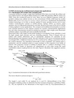
Fig. 7. Beam divergence

Considering the arrangement of a free-space optical communication link of Fig. 7, and by
invoking the thin lens approximation to the diffuse optical source whose irradiance is
represented by I
s
, the amount of optical power focused on the detector is derived as (Gowar,
1993):

ܲ
ோ
ൌ
ܫ
௦
ܣ
்
ܣ
ோ
ܮ
ଶ
ܣ
௦

(6)

A
T

and A
R
are the transmitter and receiver aperture areas while A
s
is the area of the optical
source. This clearly shows that a source with high radiance I
s
/A
s
and wide apertures are
required in order to increase the received optical power.
For a non-diffuse, small source such as the laser, the size of the image formed at the receiver
plane is no longer given by the thin lens approximation; it is determined by diffraction at the
transmitter aperture. The diffraction pattern produced by a uniformly illuminated circular
aperture of diameter, d
T
is known to consists of a set of concentric rings. The image size is
said to be diffraction limited when the radius of the first intensity minimum or dark ring of
the diffraction pattern becomes comparable in size with the diameter, d
im
of the normally
focussed image (Gowar, 1993). That is:

݀
௜௠
ൌ
ܮ
ݑ
݀
௦

൏ͳǤʹʹ
ߣܮ
݀
்

(7)
Therefore,
݀
௦
൏ͳǤʹʹ
ߣݑ
݀
்
ൎͳǤʹʹ
ߣ݂
݀
்

(8)

This equation shows that for diffraction to be the sole cause of beam divergence (diffraction
limited), the source diameter, ݀
௦
൏ͳǤʹʹ
ఒ௙
ௗ
೅
. Laser being inherently collimated and coherent
normally produces a diffraction-limited image. The diffraction limited beam divergence
angle in radian is given by ߠ

௕
؆
ఒ
ௗ
೅
.
If the transmitter and receiver effective antenna gains are respectively given by:





Ω

(9a)









(9b)
And the free-space path loss is given by:








(10)
Hence the received optical power is:










(11)









Ω


(12a)
















λ


(12b)

where the radiation solid angel Ω






. The diffraction limited beam spreading
/geometric loss in dB is thus:










λ

  



(13)

The result given by (13) can be obtained by substituting 



 for the image size in









. A beam expander of the type shown in Fig. 8, in which the diffracting aperture
has been increased, could then be used to reduce the diffraction-limited beam divergence.
Thereby reducing the beam divergence loss and increasing the received power in the
process.


Fig. 8. Beam expander diagram

However for most practical sources, the beam divergence angle is usually greater than that
dictated by diffraction. For a source with an angle of divergence, the beam size at a
TerrestrialFree-SpaceOpticalcommunications 369

Fig. 7. Beam divergence

Considering the arrangement of a free-space optical communication link of Fig. 7, and by
invoking the thin lens approximation to the diffuse optical source whose irradiance is
represented by I
s
, the amount of optical power focused on the detector is derived as (Gowar,
1993):

ܲ
ோ
ൌ
ܫ
௦
ܣ
்
ܣ
ோ

ܮ
ଶ
ܣ
௦

(6)

A
T
and A
R
are the transmitter and receiver aperture areas while A
s
is the area of the optical
source. This clearly shows that a source with high radiance I
s
/A
s
and wide apertures are
required in order to increase the received optical power.
For a non-diffuse, small source such as the laser, the size of the image formed at the receiver
plane is no longer given by the thin lens approximation; it is determined by diffraction at the
transmitter aperture. The diffraction pattern produced by a uniformly illuminated circular
aperture of diameter, d
T
is known to consists of a set of concentric rings. The image size is
said to be diffraction limited when the radius of the first intensity minimum or dark ring of
the diffraction pattern becomes comparable in size with the diameter, d
im
of the normally

focussed image (Gowar, 1993). That is:

݀
௜௠
ൌ
ܮ
ݑ
݀
௦
൏ͳǤʹʹ
ߣܮ
݀
்

(7)
Therefore,
݀
௦
൏ͳǤʹʹ
ߣݑ
݀
்
ൎͳǤʹʹ
ߣ݂
݀
்

(8)

This equation shows that for diffraction to be the sole cause of beam divergence (diffraction

limited), the source diameter, ݀
௦
൏ͳǤʹʹ
ఒ௙
ௗ
೅
. Laser being inherently collimated and coherent
normally produces a diffraction-limited image. The diffraction limited beam divergence
angle in radian is given by ߠ
௕
؆
ఒ
ௗ
೅
.
If the transmitter and receiver effective antenna gains are respectively given by:





Ω

(9a)










(9b)
And the free-space path loss is given by:







(10)
Hence the received optical power is:










(11)










Ω


(12a)
















λ


(12b)

where the radiation solid angel Ω







. The diffraction limited beam spreading
/geometric loss in dB is thus:










λ

  



(13)

The result given by (13) can be obtained by substituting 




 for the image size in








. A beam expander of the type shown in Fig. 8, in which the diffracting aperture
has been increased, could then be used to reduce the diffraction-limited beam divergence.
Thereby reducing the beam divergence loss and increasing the received power in the
process.


Fig. 8. Beam expander diagram

However for most practical sources, the beam divergence angle is usually greater than that
dictated by diffraction. For a source with an angle of divergence, the beam size at a
MobileandWirelessCommunications:Networklayerandcircuitleveldesign370
distance L away is





. The fraction of the received power to the transmitted power is
therefore be given as:
























(14)

And the geometric loss in dB thus becomes:














(15)

The beam spreading loss for the diffraction limited source given by (13) is expectedly lower
than for the non-diffraction limited case given by (15), since the image size is smaller by d
T

in the diffraction limited case.
From the foregoing, a source with very narrow divergence beam angle is preferable. It
should however be mentioned that wide divergence angles are desirable in short range FSO
links to ease the alignment requirement, compensate for building sway and eliminate the
need for active tracking systems at the expense of increased geometric loss apparently. A
typical FSO transceiver has optical beam divergence in the range of 2–10 mrad and 0.05–1.0
mrad (equivalent to a beam spread of 2–10 m, and 5 cm to 1 m, respectively at 1 km link
range) for systems without and with tracking, respectively.

3.3.1.3 Optical and window loss
This type of loss includes losses due to imperfect lenses and other optical elements used in
the design of both the transmitter and receiver. It accounts for the reflection, absorption and
scattering due to the lenses in the system (Willebrand and Ghuman, 2002). The value of the
optical loss 

can be obtained from the component manufacturer. It apparently depends on
the characteristics of the equipments and the quality of the lenses used. For FSO transceivers

installed behind windows within a building, there exists an additional optical power loss
due the window glass attenuation. Although (glass) windows allow optical signals to pass
through them, they contribute to the overall power loss of the signal. Uncoated glass
windows usually attenuate 4% per surface, because of reflection. Coated windows display
much higher losses and its magnitude is wavelength dependent.

3.3.1.4 Pointing loss
Additional power penalty is usually incurred due to lack of perfect alignment of the
transmitter and receiver. The resulting power loss is catered for by including
pointing/misalignment loss, 

in the link budget analysis. For short FSO links (< 1 km),
this might not be an issue but for longer link ranges, this can certainly not be neglected.
Misalignments could result from building sway or strong wind effect on the FOS link head
stands.

3.3.2 The link budget
Based on the losses mentioned above, the received optical power in dBm can thus be
obtained from the link budget equation as:

























(16)

The link margin, L
M
is included in the link budget equation above to cater for other losses
such as changes in specification when a faulty component is replaced, ageing of laser
sources, attenuation due to rain, snow and so on.
Figure 9 depicts the link range against
available link margin at different values of visibility for a typical commercial FSO link
whose parameters are tabulated in Table 6. In this figure, the Kim model is used in
estimating the attenuation coefficient. By operating the link under consideration at a 5 dB
link margin in clear atmosphere with over 30 km visibility, two data nodes at about 3 km
apart and running at 155 Mbps can be reliably connected with an FSO system whose
parameters are shown in Table 6.

Parameter Typical Value
Receiver aperture diameter (d

R
) 8 cm
Transmitter aperture diameter (d
T
) 2.5 cm
Beam divergence (θ) 2 mrad
Modulation technique/Bit rate On-OFF
keying/155Mbps

Transmit power 14 dBm
Receiver sensitivity -30 dBm
Optical loss (L
O
) 1 dB
Pointing loss (L
P
) 1 dB
Wavelength (λ) 850 nm
Table 6. Typical link budget parameters

One major importance of the link budget equation is in determining the achievable link
range, for a given receiver sensitivity. The receiver sensitivity by the way represents the
minimum amount of optical power needed for the system to achieve a specified level
performance; for example a bit error rate of 10
-9
. The receiver sensitivity depends on the
modulation technique in use, the noise level, fading/scintillation strength and the data rate.
Higher data rate simply implies shorter optical pulse duration, hence fewer photons that can
be detected. The noise could be from a combination of background radiation, the detection
process/quantum shot noise and the thermal noise caused by the thermal agitation of

electrons in the receiver electronic components. The theoretical receiver sensitivity at any
desired level of performance can be obtained from the analysis of Section 5.

TerrestrialFree-SpaceOpticalcommunications 371
distance L away is





. The fraction of the received power to the transmitted power is
therefore be given as:
























(14)

And the geometric loss in dB thus becomes:













(15)

The beam spreading loss for the diffraction limited source given by (13) is expectedly lower
than for the non-diffraction limited case given by (15), since the image size is smaller by d
T

in the diffraction limited case.
From the foregoing, a source with very narrow divergence beam angle is preferable. It
should however be mentioned that wide divergence angles are desirable in short range FSO

links to ease the alignment requirement, compensate for building sway and eliminate the
need for active tracking systems at the expense of increased geometric loss apparently. A
typical FSO transceiver has optical beam divergence in the range of 2–10 mrad and 0.05–1.0
mrad (equivalent to a beam spread of 2–10 m, and 5 cm to 1 m, respectively at 1 km link
range) for systems without and with tracking, respectively.

3.3.1.3 Optical and window loss
This type of loss includes losses due to imperfect lenses and other optical elements used in
the design of both the transmitter and receiver. It accounts for the reflection, absorption and
scattering due to the lenses in the system (Willebrand and Ghuman, 2002). The value of the
optical loss 

can be obtained from the component manufacturer. It apparently depends on
the characteristics of the equipments and the quality of the lenses used. For FSO transceivers
installed behind windows within a building, there exists an additional optical power loss
due the window glass attenuation. Although (glass) windows allow optical signals to pass
through them, they contribute to the overall power loss of the signal. Uncoated glass
windows usually attenuate 4% per surface, because of reflection. Coated windows display
much higher losses and its magnitude is wavelength dependent.

3.3.1.4 Pointing loss
Additional power penalty is usually incurred due to lack of perfect alignment of the
transmitter and receiver. The resulting power loss is catered for by including
pointing/misalignment loss, 

in the link budget analysis. For short FSO links (< 1 km),
this might not be an issue but for longer link ranges, this can certainly not be neglected.
Misalignments could result from building sway or strong wind effect on the FOS link head
stands.

3.3.2 The link budget
Based on the losses mentioned above, the received optical power in dBm can thus be
obtained from the link budget equation as:
























(16)

The link margin, L

M
is included in the link budget equation above to cater for other losses
such as changes in specification when a faulty component is replaced, ageing of laser
sources, attenuation due to rain, snow and so on.
Figure 9 depicts the link range against
available link margin at different values of visibility for a typical commercial FSO link
whose parameters are tabulated in Table 6. In this figure, the Kim model is used in
estimating the attenuation coefficient. By operating the link under consideration at a 5 dB
link margin in clear atmosphere with over 30 km visibility, two data nodes at about 3 km
apart and running at 155 Mbps can be reliably connected with an FSO system whose
parameters are shown in Table 6.

Parameter Typical Value
Receiver aperture diameter (d
R
) 8 cm
Transmitter aperture diameter (d
T
) 2.5 cm
Beam divergence (θ) 2 mrad
Modulation technique/Bit rate On-OFF
keying/155Mbps

Transmit power 14 dBm
Receiver sensitivity -30 dBm
Optical loss (L
O
) 1 dB
Pointing loss (L
P

) 1 dB
Wavelength (λ) 850 nm
Table 6. Typical link budget parameters

One major importance of the link budget equation is in determining the achievable link
range, for a given receiver sensitivity. The receiver sensitivity by the way represents the
minimum amount of optical power needed for the system to achieve a specified level
performance; for example a bit error rate of 10
-9
. The receiver sensitivity depends on the
modulation technique in use, the noise level, fading/scintillation strength and the data rate.
Higher data rate simply implies shorter optical pulse duration, hence fewer photons that can
be detected. The noise could be from a combination of background radiation, the detection
process/quantum shot noise and the thermal noise caused by the thermal agitation of
electrons in the receiver electronic components. The theoretical receiver sensitivity at any
desired level of performance can be obtained from the analysis of Section 5.

MobileandWirelessCommunications:Networklayerandcircuitleveldesign372

Fig. 9. Link length against available link margin for different visibility values.

3.3.3 The atmospheric turbulence effects
The temperature inhomogeneity of the atmosphere causes corresponding changes in the
index of refraction of the atmosphere resulting in eddies, cells or air packets having varying
sizes from ~0.1 cm to ~10 m. These air packets act like refractive prisms of varying indices of
refraction. The propagating optical radiation is therefore fully or partially deviated
depending on the relative size of the beam and the degree of temperature inhomogeneity
along its path. Consequently, the optical radiation traversing the turbulence atmosphere
experiences random variation/fading in its irradiance (scintillation) and phase. Familiar
effects of turbulence include the twinkling of stars caused by random fluctuations of stars’

irradiance and the shimmer of the horizon on a hot day caused by random changes in the
optical phase of the light beam resulting in the reduced image resolution (Killinger, 2002).
Atmospheric turbulence depends on i) atmospheric pressure/altitude, ii) wind speed, and
iii) variation of index of refraction due to temperature inhomogeneity. Known effects of
atmospheric turbulence include (Pratt, 1969):

a) Beam steering - Angular deviation of the beam from its original LOS causing the
beam to miss the receiver.
b) Image dancing - The received beam focus moves in the image plane due to
variations in the beam’s angle of arrival.
c) Beam spreading - Increased beam divergence due to scattering. This leads to a
reduction in received power density.
-10 -5 0 5 10 15 20 25 30 35
0
0.5
1
1.5
2
2.5
3
3.5
4
Link margin (dB)
Link Length (km)
30 km
5 km
50 km
Visibility
d) Beam scintillation - Variations in the spatial power density at the receiver plane
caused by small scale destructive interference within the optical beam.

e) Spatial coherence degradation - Turbulence also induces losses in phase coherence
across the beam phase fronts. This is particularly deleterious for photomixing (e.g.
in coherent receiver).
f) Polarisation fluctuation - This results from changes in the state of polarisation of
the received optical field after passing through a turbulent medium. However, the
amount of polarisation fluctuation is negligible for a horizontally travelling optical
radiation in atmospheric turbulence (Karp et al., 1988).

3.3.3.1 Atmospheric turbulence model
Atmospheric turbulence results from random fluctuation of the atmospheric refractive index
n along the path of a wave traversing the atmosphere. This refractive index fluctuation is the
direct product of random variations in atmospheric temperature along the wave path. The
random temperature changes themselves are a function of the altitude, h and the wind
speed, v. Scintillation causes impairment and performance degradation for long range (>
1 km) atmospheric optical communication systems. The relationship between the
temperature of the atmosphere and its refractive index is given by (Karp et al., 1988):














(17)

where P is the atmospheric pressure in millibars, and T
e
is the temperature in Kelvin.
The turbulence atmosphere can be described as containing loosely packed eddies/prisms of
varying sizes and refractive indices. The smallest eddy size l
o
is called the turbulence inner
scale, with a value of a few millimetres, while the outer scale of turbulence L
o
has its value
running to several meters. According to the Taylor’s ‘frozen-in’ model, the temporal
variation in statistical properties of the turbulent atmosphere is caused by the airmass
movement. Also, the turbulent eddies are fixed and only vary with the wind moving
perpendicularly to the direction of the traversing wave. The temporal coherence time 
o
of
atmospheric turbulence is known to be in the order of millisecond. This value is very large
compared to typical data symbol duration. Hence the terrestrial FSO channel suffers from
slow fading.
Since only the intensity modulation, direct detection laser communication systems are
discussed here, the turbulence effect of concern is the intensity fluctuation of the laser beam
traversing the atmosphere. The strength of the irradiance fluctuation in a turbulent medium
is given by the variance of the log intensity, l (also called the Roytov parameter σ
l
2
) and the
transverse coherence length of a field travelling through a turbulent channel is denoted by
ρ

o
. Over the range 





these parameters are defined as (Osche, 2002):



























(18)






(19)
TerrestrialFree-SpaceOpticalcommunications 373

Fig. 9. Link length against available link margin for different visibility values.

3.3.3 The atmospheric turbulence effects
The temperature inhomogeneity of the atmosphere causes corresponding changes in the
index of refraction of the atmosphere resulting in eddies, cells or air packets having varying
sizes from ~0.1 cm to ~10 m. These air packets act like refractive prisms of varying indices of
refraction. The propagating optical radiation is therefore fully or partially deviated
depending on the relative size of the beam and the degree of temperature inhomogeneity
along its path. Consequently, the optical radiation traversing the turbulence atmosphere
experiences random variation/fading in its irradiance (scintillation) and phase. Familiar
effects of turbulence include the twinkling of stars caused by random fluctuations of stars’
irradiance and the shimmer of the horizon on a hot day caused by random changes in the
optical phase of the light beam resulting in the reduced image resolution (Killinger, 2002).
Atmospheric turbulence depends on i) atmospheric pressure/altitude, ii) wind speed, and
iii) variation of index of refraction due to temperature inhomogeneity. Known effects of
atmospheric turbulence include (Pratt, 1969):

a) Beam steering - Angular deviation of the beam from its original LOS causing the
beam to miss the receiver.
b) Image dancing - The received beam focus moves in the image plane due to
variations in the beam’s angle of arrival.
c) Beam spreading - Increased beam divergence due to scattering. This leads to a
reduction in received power density.
-10 -5 0 5 10 15 20 25 30 35
0
0.5
1
1.5
2
2.5
3
3.5
4
Link margin (dB)
Link Length (km)
30 km
5 km
50 km
Visibility
d) Beam scintillation - Variations in the spatial power density at the receiver plane
caused by small scale destructive interference within the optical beam.
e) Spatial coherence degradation - Turbulence also induces losses in phase coherence
across the beam phase fronts. This is particularly deleterious for photomixing (e.g.
in coherent receiver).
f) Polarisation fluctuation - This results from changes in the state of polarisation of
the received optical field after passing through a turbulent medium. However, the

amount of polarisation fluctuation is negligible for a horizontally travelling optical
radiation in atmospheric turbulence (Karp et al., 1988).

3.3.3.1 Atmospheric turbulence model
Atmospheric turbulence results from random fluctuation of the atmospheric refractive index
n along the path of a wave traversing the atmosphere. This refractive index fluctuation is the
direct product of random variations in atmospheric temperature along the wave path. The
random temperature changes themselves are a function of the altitude, h and the wind
speed, v. Scintillation causes impairment and performance degradation for long range (>
1 km) atmospheric optical communication systems. The relationship between the
temperature of the atmosphere and its refractive index is given by (Karp et al., 1988):














(17)

where P is the atmospheric pressure in millibars, and T
e
is the temperature in Kelvin.

The turbulence atmosphere can be described as containing loosely packed eddies/prisms of
varying sizes and refractive indices. The smallest eddy size l
o
is called the turbulence inner
scale, with a value of a few millimetres, while the outer scale of turbulence L
o
has its value
running to several meters. According to the Taylor’s ‘frozen-in’ model, the temporal
variation in statistical properties of the turbulent atmosphere is caused by the airmass
movement. Also, the turbulent eddies are fixed and only vary with the wind moving
perpendicularly to the direction of the traversing wave. The temporal coherence time 
o
of
atmospheric turbulence is known to be in the order of millisecond. This value is very large
compared to typical data symbol duration. Hence the terrestrial FSO channel suffers from
slow fading.
Since only the intensity modulation, direct detection laser communication systems are
discussed here, the turbulence effect of concern is the intensity fluctuation of the laser beam
traversing the atmosphere. The strength of the irradiance fluctuation in a turbulent medium
is given by the variance of the log intensity, l (also called the Roytov parameter σ
l
2
) and the
transverse coherence length of a field travelling through a turbulent channel is denoted by
ρ
o
. Over the range 






these parameters are defined as (Osche, 2002):


























(18)







(19)
MobileandWirelessCommunications:Networklayerandcircuitleveldesign374
where C
n
2
is the refractive index structure constant (which characterizes the strength of
refractive index variation in the medium). A commonly used model for C
n
2
is the Hufnagel-
Valley (H-V) model described by the following (Andrews et al., 2001):





















 

   



 

 

  

(20)

 is taken as the nominal value of C
n
2
(0) at ground level in m
-2/3
. Generally, the structure
parameter is assumed constant for a horizontal link and ranges from 10
-15
m

-2/3
for weak to
10
-12
m
-2/3
for strong turbulence regimes.
Considering single scattering characterized weak turbulence and assuming the log intensity
l of laser light traversing the turbulent atmosphere to be normally distributed, that is
σ


σ


, then the probability density function (pdf) of the laser beam intensity,






is given by:









σ








 

 
σ





σ



(21)

where I
o
is the mean received intensity without turbulence. The normalised variance of the
intensity σ



is derived as follows:





























  
(22)

The turbulence model discussed thus far is the lognormal turbulence, it is only valid for
the weak turbulence with σ
N
2
< 1.2. For σ


, saturation sets in and the model no longer
holds. Turbulence induced irradiance fluctuation can enter saturation due to one or a
combination of increased C
n
, link length and reduced wavelength. Also, when multiple
scatterings are experienced especially in longer link ranges, the incident wave becomes
increasingly incoherent and log normal model becomes invalid. Though not discussed here,
another model which has a wider range of validity but lacks the mathematical simplicity of
lognormal is the gamma-gamma turbulence model. Moreover, in the limit of strong
irradiance fluctuations (i.e. in saturation regime and beyond) where the link length spans
several kilometres, the number of independent scatterings becomes large (Karp et al., 1988).
In the saturation regime, irradiance fluctuation is believed to follow the negative
exponential distribution.

4. Noise Sources
Background noise: This is due to radiations from both the sky (extended source) and the Sun
(localised source). Background radiation from other celestial bodies such as stars and
reflected background radiation are assumed too weak to be considered for terrestrial FSO
links, they however contribute significantly to background noise in deep space FSO systems.
The irradiance (power per unit area) expressions for both the extended and the localised

background sources are given by the following equations:










(23)




(24)

where N(λ) and W(λ) are the spectral radiance of the sky and spectral radiant emittance of
the Sun, respectively, Δλ is the bandwidth of the optical BPF at the receiver, and Ω is the
receiver FOV in radian. By carefully choosing a receiver with a very narrow FOV and Δλ,
the impact of background noise can be greatly reduced. Optical BPF in the form of coatings
on the receiver optics/telescope with Δλ < 1 nm are now readily available. Empirical values
of N(λ) and W(λ) under different observation conditions are also available in reference
(Gagliardi and Karp, 1995). The background noise is a shot noise and its variance is given
by:










(25)

where B is the system electrical bandwidth and  = ηqλ/hc is the photodetector
responsivity, η is the detector quantum efficiency, q is the electronic charge; h and c
represent the Plank’s constant and the speed of light in vacuum, respectively.
Quantum noise: A shot noise due to the statistical nature of the optical detection process. Its
value is usually very small with variance:





(26)

Thermal noise: This is the noise caused by the thermal fluctuations of electrons in a receiver
circuit of equivalent resistance R
L
, and temperature T
e
. Its variance is given by:












(27)

The dark current and the relative intensity noise are usually so small and negligible. The
total noise variance is thus given as:













(28)
TerrestrialFree-SpaceOpticalcommunications 375
where C
n
2
is the refractive index structure constant (which characterizes the strength of
refractive index variation in the medium). A commonly used model for C

n
2
is the Hufnagel-
Valley (H-V) model described by the following (Andrews et al., 2001):




















 

   




 

 

  

(20)

 is taken as the nominal value of C
n
2
(0) at ground level in m
-2/3
. Generally, the structure
parameter is assumed constant for a horizontal link and ranges from 10
-15
m
-2/3
for weak to
10
-12
m
-2/3
for strong turbulence regimes.
Considering single scattering characterized weak turbulence and assuming the log intensity
l of laser light traversing the turbulent atmosphere to be normally distributed, that is
σ


σ



, then the probability density function (pdf) of the laser beam intensity,






is given by:








σ








 

 

σ





σ



(21)

where I
o
is the mean received intensity without turbulence. The normalised variance of the
intensity σ


is derived as follows:





























  
(22)

The turbulence model discussed thus far is the lognormal turbulence, it is only valid for
the weak turbulence with σ
N
2
< 1.2. For σ


, saturation sets in and the model no longer
holds. Turbulence induced irradiance fluctuation can enter saturation due to one or a
combination of increased C

n
, link length and reduced wavelength. Also, when multiple
scatterings are experienced especially in longer link ranges, the incident wave becomes
increasingly incoherent and log normal model becomes invalid. Though not discussed here,
another model which has a wider range of validity but lacks the mathematical simplicity of
lognormal is the gamma-gamma turbulence model. Moreover, in the limit of strong
irradiance fluctuations (i.e. in saturation regime and beyond) where the link length spans
several kilometres, the number of independent scatterings becomes large (Karp et al., 1988).
In the saturation regime, irradiance fluctuation is believed to follow the negative
exponential distribution.

4. Noise Sources
Background noise: This is due to radiations from both the sky (extended source) and the Sun
(localised source). Background radiation from other celestial bodies such as stars and
reflected background radiation are assumed too weak to be considered for terrestrial FSO
links, they however contribute significantly to background noise in deep space FSO systems.
The irradiance (power per unit area) expressions for both the extended and the localised
background sources are given by the following equations:










(23)





(24)

where N(λ) and W(λ) are the spectral radiance of the sky and spectral radiant emittance of
the Sun, respectively, Δλ is the bandwidth of the optical BPF at the receiver, and Ω is the
receiver FOV in radian. By carefully choosing a receiver with a very narrow FOV and Δλ,
the impact of background noise can be greatly reduced. Optical BPF in the form of coatings
on the receiver optics/telescope with Δλ < 1 nm are now readily available. Empirical values
of N(λ) and W(λ) under different observation conditions are also available in reference
(Gagliardi and Karp, 1995). The background noise is a shot noise and its variance is given
by:









(25)

where B is the system electrical bandwidth and  = ηqλ/hc is the photodetector
responsivity, η is the detector quantum efficiency, q is the electronic charge; h and c
represent the Plank’s constant and the speed of light in vacuum, respectively.
Quantum noise: A shot noise due to the statistical nature of the optical detection process. Its
value is usually very small with variance:





(26)

Thermal noise: This is the noise caused by the thermal fluctuations of electrons in a receiver
circuit of equivalent resistance R
L
, and temperature T
e
. Its variance is given by:











(27)

The dark current and the relative intensity noise are usually so small and negligible. The
total noise variance is thus given as:














(28)