New Developments in Biomedical Engineering 2011 Part 2 doc

Bạn đang xem bản rút gọn của tài liệu. Xem và tải ngay bản đầy đủ của tài liệu tại đây (1.8 MB, 40 trang )

NewDevelopmentsinBiomedicalEngineering32
val of 1s, 85% of the stimuli at 800Hz and randomly presented 15% deviant tones at 560Hz.
The subject was sitting in a chair and was asked to press a button every time he heard the
deviant target tone. The sampling rate of the EEG was 500 Hz. From the recordings, channel
Cz was selected for analysis, after bandpass ﬁltering in the range 1-40Hz. Average responses
from the two conditions are shown in Figure 2 (Section 2). For investigation of the single trial
variability of the P300 peak, EEG epochs from -100 ms to 600 ms relative to the stimulus onset
of each deviant stimulus were here used.
The model was designed as in section 7.1 but now for the slower P300 wave the selection f
c
=
10Hz was made. The application of the empirical rule (27) gave in this case k = 15. Kalman
smoother estimates were computed with the selection σ
2
ω
= 9, with respect to the expected
faster variability of the potential.
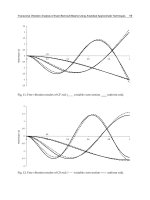
In Figure 5 (I) there are presented the EP measurements in the original stimulus order (trial-by-
trial). In the same ﬁgure (II) the obtained estimates based on the measurements (I) are shown.
Clearly, in the estimates, the dynamic variability of the P300 peak potential is revealed, sug-
gesting that it cannot be considered as occurring at ﬁxed latency from the stimuli presentation.
At the same image (II), the estimated latency is also plotted as a function of the consecutive
trial t. The latency of the peak was estimated from the Kalman smoother estimates based on
the maximum value within the time interval 250-370ms after the presentation of the stimuli.
The estimated time-varying latency of the P300 peak was then used to order the single-trial
measurements. The sorted single-trials (condition-by-condition) are shown at Figure 5 (III).
The shorted latency estimates are plotted again over the image plot. This plot clearly demon-
strates that the latency estimates obtained with Kalman smoother are of acceptable accuracy.
Finally, the algorithm was also applied to the sorted measurements (III). The value σ
2

ω
=
4 was selected and new point estimates for the latency were obtained as before. Kalman
smoother estimates and the new latency estimates are plotted in Figure 5 (IV). The linear trend
of the sorted potentials allows the use of even smaller value for state-noise variance parameter
(Georgiadis et al., 2005b), thus reducing even more the noise without reducing the variability
of the peak. The last obtained estimates of the latencies were plotted over the original non
sorted measurements (I). The similarities between the estimated latency ﬂuctuations in (I)
and (II) underline the robustness of the method.
8. Conclusion and Future Directions
EP research has to deal with several inherent difﬁculties. Traditional analysis is based on aver-
aged data often by forming extra grand averages of different populations. Thus, trial-to-trial
variability and individual subject characteristics are largely ignored (Fell, 2007). Therefore,
the study of isolated components retrieved by averages might be misleading, or at least it is
a simpliﬁcation of the reality. For example, habituation may occur and the responses could
be different from the beginning to the end of the recording session. Furthermore, cognitive
potentials exhibit rich latency and amplitude variability that traditional research based on av-
eraging is not able to exploit for studying complex cognitive processes. Latency variability
could be used, for instance, for studying perceptual changes, quantifying stimulus classiﬁca-
tion speed or task difﬁculty.
In this chapter, state-space modeling for single-trial estimation of EPs was presented in its
general form based on Bayesian estimation theory. This formulation enables the selection
of different models for dynamical estimation. In general, the applicability of the proposed
Fig. 5. Single-trial EP latency variability.
State-spacemodelingforsingle-trialevokedpotentialestimation 33
val of 1s, 85% of the stimuli at 800Hz and randomly presented 15% deviant tones at 560Hz.
The subject was sitting in a chair and was asked to press a button every time he heard the
deviant target tone. The sampling rate of the EEG was 500 Hz. From the recordings, channel
Cz was selected for analysis, after bandpass ﬁltering in the range 1-40Hz. Average responses
from the two conditions are shown in Figure 2 (Section 2). For investigation of the single trial

variability of the P300 peak, EEG epochs from -100 ms to 600 ms relative to the stimulus onset
of each deviant stimulus were here used.
The model was designed as in section 7.1 but now for the slower P300 wave the selection f
c
=
10Hz was made. The application of the empirical rule (27) gave in this case k = 15. Kalman
smoother estimates were computed with the selection σ
2
ω
= 9, with respect to the expected
faster variability of the potential.
In Figure 5 (I) there are presented the EP measurements in the original stimulus order (trial-by-
trial). In the same ﬁgure (II) the obtained estimates based on the measurements (I) are shown.
Clearly, in the estimates, the dynamic variability of the P300 peak potential is revealed, sug-
gesting that it cannot be considered as occurring at ﬁxed latency from the stimuli presentation.
At the same image (II), the estimated latency is also plotted as a function of the consecutive
trial t. The latency of the peak was estimated from the Kalman smoother estimates based on
the maximum value within the time interval 250-370ms after the presentation of the stimuli.
The estimated time-varying latency of the P300 peak was then used to order the single-trial
measurements. The sorted single-trials (condition-by-condition) are shown at Figure 5 (III).
The shorted latency estimates are plotted again over the image plot. This plot clearly demon-
strates that the latency estimates obtained with Kalman smoother are of acceptable accuracy.
Finally, the algorithm was also applied to the sorted measurements (III). The value σ
2
ω
=
4 was selected and new point estimates for the latency were obtained as before. Kalman
smoother estimates and the new latency estimates are plotted in Figure 5 (IV). The linear trend
of the sorted potentials allows the use of even smaller value for state-noise variance parameter
(Georgiadis et al., 2005b), thus reducing even more the noise without reducing the variability

of the peak. The last obtained estimates of the latencies were plotted over the original non
sorted measurements (I). The similarities between the estimated latency ﬂuctuations in (I)
and (II) underline the robustness of the method.
8. Conclusion and Future Directions
EP research has to deal with several inherent difﬁculties. Traditional analysis is based on aver-
aged data often by forming extra grand averages of different populations. Thus, trial-to-trial
variability and individual subject characteristics are largely ignored (Fell, 2007). Therefore,
the study of isolated components retrieved by averages might be misleading, or at least it is
a simpliﬁcation of the reality. For example, habituation may occur and the responses could
be different from the beginning to the end of the recording session. Furthermore, cognitive
potentials exhibit rich latency and amplitude variability that traditional research based on av-
eraging is not able to exploit for studying complex cognitive processes. Latency variability
could be used, for instance, for studying perceptual changes, quantifying stimulus classiﬁca-
tion speed or task difﬁculty.
In this chapter, state-space modeling for single-trial estimation of EPs was presented in its
general form based on Bayesian estimation theory. This formulation enables the selection
of different models for dynamical estimation. In general, the applicability of the proposed
Fig. 5. Single-trial EP latency variability.
NewDevelopmentsinBiomedicalEngineering34
methodology primarily relates on the assumption of hidden dynamic variability from trial-to-
trial or from condition-to-condition. A practical method for designing an observation model
was also presented and its capability to reveal meaningful amplitude and latency ﬂuctuations
in EP measurements was demonstrated. In the approach, optimal estimates for the states
are obtained with Kalman ﬁlter and smoother algorithms. When all the measurements are
available (batch processing) Kalman smoother should be used.
EPs also contain rich spatial information that can be used for describing brain dynamics
(Makeig et al., 2004; Ranta-aho et al., 2003). In this study, this important issue was not dis-
cussed and emphasis was given on optimal estimation of some temporal EP characteristics.
Future development of the presented methodology involves the extension of the approach
to multichannel and multimodal data sets, for instance, simultaneously measured EEG/ERP

and fMRI/BOLD signals (Debener et al., 2006), for the study of dynamic changes of the central
nervous system.
Acknowledgments
The authors acknowledge ﬁnancial support from the Academy of Finland (project numbers:
123579, 1.1.2008-31.12.2011, and 126873, 1.1.2009-31.12.2011).
9. References
Cerutti, S., Bersani, V., Carrara, A. & Liberati, D. (1987). Analysis of visual evoked potentials
through Wiener ﬁltering applied to a small number of sweeps, Journal of Biomedical
Engineering 9(1): 3–12.
Debener, S., Ullsperger, M., Siegel, M. & Engel, A. (2006). Single-trial EEG-fMRI reveals the
dynamics of cognitive function, Trends in Cognitive Sciences 10(2): 558–63.
Delorme, A. & Makeig, S. (2004). EEGLAB: an open source toolbox for analysis of single-trial
EEG dynamics including independent component analysis, Journal of Neuroscience
Methods 134(1): 9–21.
Doncarli, C., Goering, L. & Guiheneuc, P. (1992). Adaptive smoothing of evoked potentials,
Signal Processing 28(1): 63–76.
Fell, J. (2007). Cognitive neurophysiology: Beyond averaging, NeuroImage 37: 1069–1027.
Georgiadis, S. (2007). State-Space Modeling and Bayesian Methods for Evoked Potential Estimation,
PhD thesis, Kuopio University Publications C. Natural and Environmental Sciences
213. (available: .ﬁ/).
Georgiadis, S., Ranta-aho, P., Tarvainen, M. & Karjalainen, P. (2005a). Recursive mean square
estimators for single-trial event related potentials, Proc. Finnish Signal Processing Sym-
posium - FINSIG’05, Kuopio, Finland.
Georgiadis, S., Ranta-aho, P., Tarvainen, M. & Karjalainen, P. (2005b). Single-trial dynamical
estimation of event related potentials: a Kalman ﬁlter based approach, IEEE Transac-
tions on Biomedical Engineering 52(8): 1397–1406.
Georgiadis, S., Ranta-aho, P., Tarvainen, M. & Karjalainen, P. (2007). A subspace method for
dynamical estimation of evoked potentials, Computational Intelligence and Neuroscience
2007: Article ID 61916, 11 pages.
Georgiadis, S., Ranta-aho, P., Tarvainen, M. & Karjalainen, P. (2008). Tracking single-trial

evoked potential changes with Kalman ﬁltering and smoothing, 30th Annual Inter-
national Conference of the IEEE Engineering in Medicine and Biology Society, Vancouver,
Canada, pp. 157–160.
Holm, A., Ranta-aho, P., Sallinen, M., Karjalainen, P. & Müller, K. (2006). Relationship of P300
single trial responses with reaction time and preceding stimulus sequence, Interna-
tional Journal of Psychophysiology 61(2): 244–252.
Intriligator, J. & Polich, J. (1994). On the relationship between background EEG and the P300
event-related potential, Biological Psychology 37(3): 207–218.
Jansen, B., Agarwal, G., Hegde, A. & Boutros, N. (2003). Phase synchronization of the ongoing
EEG and auditory EP generation, Clinical Neurophysiology 114(1): 79–85.
Kaipio, J. & Somersalo, E. (2005). Statistical and Computational Inverse Problems, Applied Math-
ematical Sciences, Springer.
Kalman, R. (1960). A new approach to linear ﬁltering and prediction problems, Transactions of
the ASME, Journal of Basic Engineering 82: 35–45.
Karjalainen, P., Kaipio, J., Koistinen, A. & Vauhkonen, M. (1999). Subspace regularization
method for the single trial estimation of evoked potentials, IEEE Transactions on
Biomedical Engineering 46(7): 849–860.
Knuth, K., Shah, A., Truccolo, W., Ding, M., Bressler, S. & Schroeder, C. (2006). Differentially
variable component analysis (dVCA): Identifying multiple evoked components us-
ing trial-to-trial variability, Journal of Neurophysiology 95(5): 3257–3276.
Li, R., Principe, J., Bradley, M. & Ferrari, V. (2009). A spatiotemporal ﬁltering methodology for
single-trial ERP component estimation, IEEE Transactions on Biomedical Engineering
56(1): 83–92.
Makeig, S., Debener, S. & Delorme, A. (2004). Mining event-related brain dynamics, Trends in
Cognitive Science 8(5): 204–210.
Makeig, S., Westerﬁeld, M., Jung, T P., Enghoff, S., Townsend, J., Courchesne, E. & Sejnowski,
T. (2002). Dynamic brain sources of visual evoked responses, Science 295: 690–694.
Mäkinen, V., Tiitinen, H. & May, P. (2005). Auditory even-related responses are generated
independently of ongoing brain activity, NeuroImage 24(4): 961–968.
Malmivuo, J. & Plonsey, R. (1995). Bioelectromagnetism, Oxford university press, New York.

Niedermeyer, E. & da Silva, F. L. (eds) (1999). Electroencephalography: Basic Principles, Clinical
Applications, and Related Fields, 4th edn, Williams and Wilkins.
Qiu, W., Chang, C., Lie, W., Poon, P., Lam, F., Hamernik, R., Wei, G. & Chan, F. (2006). Real-
time data-reusing adaptive learning of a radial basis function network for tracking
evoked potentials, IEEE Transanctions on Biomedical Engineering 53(2): 226–237.
Quiroga, R. Q. & Garcia, H. (2003). Single-trial evoked potentials with wavelet denoising,
Clinical Neurophysiology 114: 376–390.
Ranta-aho, P., Koistinen, A., Ollikainen, J., Kaipio, J., Partanen, J. & Karjalainen, P. (2003).
Single-trial estimation of multichannel evoked-potential measurements, IEEE Trans-
actions on Biomedical Engineering 50(2): 189–196.
Rauch, H., Tung, F. & Striebel, C. (1965). Maximum likelihood estimates of linear dynamic
systems, AIAA Journal 3: 1445–1450.
Sorenson, H. (1980). Parameter Estimation, Principles and Problems, Vol. 9 of Control and Systems
Theory, Marcel Dekker Inc., New York.
Thakor, N., Vaz, C., McPherson, R. & Hanley, D. F. (1991). Adaptive Fourier series modeling of
time-varying evoked potentials: Study of human somatosensory evoked response to
etomidate anesthetic, Electroencephalography and Clinical Neurophysiology 80(2): 108–
118.
State-spacemodelingforsingle-trialevokedpotentialestimation 35
methodology primarily relates on the assumption of hidden dynamic variability from trial-to-
trial or from condition-to-condition. A practical method for designing an observation model
was also presented and its capability to reveal meaningful amplitude and latency ﬂuctuations
in EP measurements was demonstrated. In the approach, optimal estimates for the states
are obtained with Kalman ﬁlter and smoother algorithms. When all the measurements are
available (batch processing) Kalman smoother should be used.
EPs also contain rich spatial information that can be used for describing brain dynamics
(Makeig et al., 2004; Ranta-aho et al., 2003). In this study, this important issue was not dis-
cussed and emphasis was given on optimal estimation of some temporal EP characteristics.
Future development of the presented methodology involves the extension of the approach
to multichannel and multimodal data sets, for instance, simultaneously measured EEG/ERP

Niedermeyer, E. & da Silva, F. L. (eds) (1999). Electroencephalography: Basic Principles, Clinical
Applications, and Related Fields, 4th edn, Williams and Wilkins.
Qiu, W., Chang, C., Lie, W., Poon, P., Lam, F., Hamernik, R., Wei, G. & Chan, F. (2006). Real-
time data-reusing adaptive learning of a radial basis function network for tracking
evoked potentials, IEEE Transanctions on Biomedical Engineering 53(2): 226–237.
Quiroga, R. Q. & Garcia, H. (2003). Single-trial evoked potentials with wavelet denoising,
Clinical Neurophysiology 114: 376–390.
Ranta-aho, P., Koistinen, A., Ollikainen, J., Kaipio, J., Partanen, J. & Karjalainen, P. (2003).
Single-trial estimation of multichannel evoked-potential measurements, IEEE Trans-
actions on Biomedical Engineering 50(2): 189–196.
Rauch, H., Tung, F. & Striebel, C. (1965). Maximum likelihood estimates of linear dynamic
systems, AIAA Journal 3: 1445–1450.
Sorenson, H. (1980). Parameter Estimation, Principles and Problems, Vol. 9 of Control and Systems
Theory, Marcel Dekker Inc., New York.
Thakor, N., Vaz, C., McPherson, R. & Hanley, D. F. (1991). Adaptive Fourier series modeling of
time-varying evoked potentials: Study of human somatosensory evoked response to
etomidate anesthetic, Electroencephalography and Clinical Neurophysiology 80(2): 108–
118.
NewDevelopmentsinBiomedicalEngineering36
Truccolo, W., Mingzhou, D., Knuth, K., Nakamura, R. & Bressler, S. (2002). Trial-to-trial vari-
ability of cortical evoked responses: implications for the analysis of functional con-
nectivity, Clinical Neurophysiology 113(2): 206–226.
Turetsky, B., Raz, J. & Fein, G. (1989). Estimation of trial-to-trial variation in evoked potential
signals by smoothing across trials, Psychophysiology 26(6): 700–712.
Non-StationaryBiosignalModelling 37
Non-StationaryBiosignalModelling
CarlosS.Lima,AdrianoTavares,JoséH.Correia,ManuelJ.CardosoandDanielBarbosa
X

Non-Stationary Biosignal Modelling

Carlos S. Lima, Adriano Tavares, José H. Correia,
Manuel J. Cardoso
1
and Daniel Barbosa
University of Minho
Portugal
1
University College of London
England

1. Introduction
Signals of biomedical nature are in the most cases characterized by short, impulse-like
events that represent transitions between different phases of a biological cycle. As an
example hearth sounds are essentially events that represent transitions between the
different hemodynamic phases of the cardiac cycle. Classical techniques in general analyze
the signal over long periods thus they are not adequate to model impulse-like events. High
variability and the very often necessity to combine features temporally well localized with
others well localized in frequency remains perhaps the most important challenges not yet
completely solved for the most part of biomedical signal modeling. Wavelet Transform
(WT) provides the ability to localize the information in the time-frequency plane; in
particular, they are capable of trading on type of resolution for the other, which makes them
especially suitable for the analysis of non-stationary signals.
State of the art automatic diagnosis algorithms usually rely on pattern recognition based
approaches. Hidden Markov Models (HMM’s) are statistically based pattern recognition
techniques with the ability to break a signal in almost stationary segments in a framework
known as quasi-stationary modeling. In this framework each segment can be modeled by
classical approaches, since the signal is considered stationary in the segment, and at a whole
a quasi-stationary approach is obtained.
Recently Discrete Wavelet Transform (DWT) and HMM’s have been combined as an effort

to increase the accuracy of pattern recognition based approaches regarding automatic
diagnosis purposes. Two main motivations have been appointed to support the approach.
Firstly, in each segment the signal can not be exactly stationary and in this situation the
DWT is perhaps more appropriate than classical techniques that usually considers
stationarity. Secondly, even if the process is exactly stationary over the entire segment the
capacity given by the WT of simultaneously observing the signal at various scales (at
different levels of focus), each one emphasizing different characteristics can be very
beneficial regarding classification purposes.
This chapter presents an overview of the various uses of the WT and HMM’s in Computer
Assisted Diagnosis (CAD) in medicine. Their most important properties regarding
biomedical applications are firstly described. The analogy between the WT and some of the
3
NewDevelopmentsinBiomedicalEngineering38

biological processing that occurs in the early components of the visual and auditory
systems, which partially supports the WT applications in medicine is shortly described. The
use of the WT in the analyses of 1-D physiological signals especially electrocardiography
(ECG) and phonocardiography (PCG) are then reviewed. A survey of recent wavelet
developments in medical imaging is then provided. These include biomedical image
processing algorithms as noise reduction, image enhancement and detection of micro-
calcifications in mammograms, image reconstruction and acquisition schemes as
tomography and Magnetic Resonance Imaging (MRI), and multi-resolution methods for the
registration and statistical analysis of functional images of the brain as positron emission
tomography (PET) and functional MRI.
The chapter provides an almost complete theoretical explanation of HMMs. Then a review
of HMMs in electrocardiography and phonocardiography is given. Finally more recent
approaches involving both WT and HMMs specifically in electrocardiography and
phonocardiography are reviewed.

2. Wavelets and biomedical signals

Biomedical applications usually require most sophisticated signal processing techniques
than others fields of engineering. The information of interest is often a combination of
features that are well localized in space and time. Some examples are spikes and transients
in electroencephalograph signals and microcalcifications in mammograms and others more
diffuse as texture, small oscillations and bursts. This universe of events at opposite extremes
in the time-frequency localization can not be efficiently handled by classical signal
processing techniques mostly based on the Fourier analysis. In the past few years,
researchers from mathematics and signal processing have developed the concept of
multiscale representation for signal analysis purposes (Vetterli & Kovacevic, 1995). These
wavelet based representations have over the traditional Fourier techniques the advantage of
localize the information in the time-frequency plane. They are capable of trading one type of
resolution for the other, which makes them especially suitable for modelling non-stationary
events. Due to these characteristics of the WT and the difficult conditions frequently
encountered in biomedical signal analysis, WT based techniques proliferated in medical
applications ranging from the more traditional physiological signals such as ECG to the
most recent imaging modalities as PET and MRI. Theoretically wavelet analysis is a
reasonably complicated mathematical discipline, at least for most biomedical engineers, and
consequently a detailed analysis of this technique is out of the scope of this chapter. The
interested reader can find detailed references such as (Vetterli & Kovacevic, 1995) and
(Mallat, 1998). The purpose of this chapter is only to emphasize the wavelet properties more
related to current biomedical applications.

2.1 The wavelet transform - An overview
The wavelet transform (WT) is a signal representation in a scale-time space, where each
scale represents a focus level of the signal and therefore can be seen as a result of a band-
pass filtering.
Given a time-varying signal x(t), WTs are a set of coefficients that are inner products of the
signal with a family of wavelets basis functions obtained from a standard function known as

mother wavelet. In Continuous Wavelet Transform (CWT) the wavelet corresponding to scale

s and time location τ is given by

(1)

where ψ(t) is the mother wavelet, which can be viewed as a band-pass function. The term
s ensures energy preservation. In the CWT the time-scale parameters vary continuously.
The wavelet transform of a continuous time varying signal x(t) is given by

(2)

where the asterisk stands for complex conjugate. Equation (2) shows that the WT is the
convolution between the signal and the wavelet function at scale s. For a fixed value of the
scale parameter s, the WT which is now a function of the continuous shift parameter τ, can
be written as a convolution equation where the filter corresponds to a rescaled and time-
reversed version of the wavelet as shown by equation (1) setting t=0. From the time scaling
property of the Fourier Transform the frequency response of the wavelet filter is given by

(3)

One important property of the wavelet filter is that for a discrete set of scales, namely the
dyadic scale
i
s 2 a constant-Q filterbank is obtained, where the quality factor of the filter is
defined as the central frequency to bandwidth ratio. Therefore WT provides a
decomposition of a signal into subbands with a bandwidth that increases linearly with the

frequency. Under this framework the WT can be viewed as a special kind of spectral
analyser. Energy estimates in different bands or related measures can discriminate between
various physiological states (Akay & al. 1994). Under this approach, the purpose is to
analyse turbulent hearth sounds to detect coronary artery disease. The purpose of the
approach followed by (Akay & Szeto 1994) is to characterize the states of fetal electrocortical
activity. However, this type of global feature extraction assumes stationarity, therefore
similar results can also be obtained using more conventional Fourier techniques. Wavelets
viewed as a filterbank have motivated several approaches based on reversible wavelet
decomposition such as noise reduction and image enhancement algorithms. The principle is
to handle selectively the wavelet components prior to reconstruction. (Mallat & Zhong,
1992) used such a filterbank system to obtain a multiscale edge representation of a signal
from its wavelets maxima. They proposed an iterative algorithm that reconstructs a very
close approximation of the original from this subset of features. This approach has been
adapted for noise reduction in evoked response potentials and in MR images and also in
image enhancement regarding the detection of microcalcifications in mammograms.










 dt
s
t
tx
s

s
x



*
)(
1
),(








s
t
s
s



1
,
 

sΨs
s

τ
ψ
s
1
*








Non-StationaryBiosignalModelling 39

biological processing that occurs in the early components of the visual and auditory
systems, which partially supports the WT applications in medicine is shortly described. The
use of the WT in the analyses of 1-D physiological signals especially electrocardiography
(ECG) and phonocardiography (PCG) are then reviewed. A survey of recent wavelet
developments in medical imaging is then provided. These include biomedical image
processing algorithms as noise reduction, image enhancement and detection of micro-
calcifications in mammograms, image reconstruction and acquisition schemes as
tomography and Magnetic Resonance Imaging (MRI), and multi-resolution methods for the
registration and statistical analysis of functional images of the brain as positron emission
tomography (PET) and functional MRI.
The chapter provides an almost complete theoretical explanation of HMMs. Then a review
of HMMs in electrocardiography and phonocardiography is given. Finally more recent
approaches involving both WT and HMMs specifically in electrocardiography and
phonocardiography are reviewed.

2. Wavelets and biomedical signals
Biomedical applications usually require most sophisticated signal processing techniques
than others fields of engineering. The information of interest is often a combination of
features that are well localized in space and time. Some examples are spikes and transients
in electroencephalograph signals and microcalcifications in mammograms and others more
diffuse as texture, small oscillations and bursts. This universe of events at opposite extremes
in the time-frequency localization can not be efficiently handled by classical signal
processing techniques mostly based on the Fourier analysis. In the past few years,
researchers from mathematics and signal processing have developed the concept of
multiscale representation for signal analysis purposes (Vetterli & Kovacevic, 1995). These
wavelet based representations have over the traditional Fourier techniques the advantage of
localize the information in the time-frequency plane. They are capable of trading one type of
resolution for the other, which makes them especially suitable for modelling non-stationary
events. Due to these characteristics of the WT and the difficult conditions frequently
encountered in biomedical signal analysis, WT based techniques proliferated in medical
applications ranging from the more traditional physiological signals such as ECG to the
most recent imaging modalities as PET and MRI. Theoretically wavelet analysis is a
reasonably complicated mathematical discipline, at least for most biomedical engineers, and
consequently a detailed analysis of this technique is out of the scope of this chapter. The
interested reader can find detailed references such as (Vetterli & Kovacevic, 1995) and
(Mallat, 1998). The purpose of this chapter is only to emphasize the wavelet properties more
related to current biomedical applications.

2.1 The wavelet transform - An overview
The wavelet transform (WT) is a signal representation in a scale-time space, where each
scale represents a focus level of the signal and therefore can be seen as a result of a band-
pass filtering.
Given a time-varying signal x(t), WTs are a set of coefficients that are inner products of the
signal with a family of wavelets basis functions obtained from a standard function known as

mother wavelet. In Continuous Wavelet Transform (CWT) the wavelet corresponding to scale
s and time location τ is given by

(1)

where ψ(t) is the mother wavelet, which can be viewed as a band-pass function. The term
s ensures energy preservation. In the CWT the time-scale parameters vary continuously.
The wavelet transform of a continuous time varying signal x(t) is given by

(2)

where the asterisk stands for complex conjugate. Equation (2) shows that the WT is the
convolution between the signal and the wavelet function at scale s. For a fixed value of the
scale parameter s, the WT which is now a function of the continuous shift parameter τ, can
be written as a convolution equation where the filter corresponds to a rescaled and time-
reversed version of the wavelet as shown by equation (1) setting t=0. From the time scaling
property of the Fourier Transform the frequency response of the wavelet filter is given by

(3)

One important property of the wavelet filter is that for a discrete set of scales, namely the
dyadic scale
i
s 2 a constant-Q filterbank is obtained, where the quality factor of the filter is
defined as the central frequency to bandwidth ratio. Therefore WT provides a

decomposition of a signal into subbands with a bandwidth that increases linearly with the
frequency. Under this framework the WT can be viewed as a special kind of spectral
analyser. Energy estimates in different bands or related measures can discriminate between
various physiological states (Akay & al. 1994). Under this approach, the purpose is to
analyse turbulent hearth sounds to detect coronary artery disease. The purpose of the
approach followed by (Akay & Szeto 1994) is to characterize the states of fetal electrocortical
activity. However, this type of global feature extraction assumes stationarity, therefore
similar results can also be obtained using more conventional Fourier techniques. Wavelets
viewed as a filterbank have motivated several approaches based on reversible wavelet
decomposition such as noise reduction and image enhancement algorithms. The principle is
to handle selectively the wavelet components prior to reconstruction. (Mallat & Zhong,
1992) used such a filterbank system to obtain a multiscale edge representation of a signal
from its wavelets maxima. They proposed an iterative algorithm that reconstructs a very
close approximation of the original from this subset of features. This approach has been
adapted for noise reduction in evoked response potentials and in MR images and also in
image enhancement regarding the detection of microcalcifications in mammograms.










 dt
s
t
tx

s
s
x



*
)(
1
),(








s
t
s
s



1
,
 

sΨs

s
τ
ψ
s
1
*








NewDevelopmentsinBiomedicalEngineering40

From the filterbank point of view the shape of the mother wavelet seems to be important in
order to emphasize some signal characteristics, however this topic is not explored in the
ambit of the present chapter.
Regarding implementation issues both s and τ must be discretized. The most usual way to
sample the time-scale plane is on a so-called dyadic grid, meaning that sampled points in the
time-scale plane are separated by a power of two. This procedure leads to an increase in
computational efficiency for both WT and Inverse Wavelet Transform (IWT). Under this
constraint the Discrete Wavelet Transform (DWT) is defined as

(4)

which means that DWT coefficients are sampled from CWT coefficients. As a dyadic scale is

used and therefore s
0
=2 and τ
0
=1, yielding s=2
j
and τ=k2
j
where j and k are integers.
As the scale represents the level of focus from the which the signal is viewed, which is
related to the frequency range involved, the digital filter banks are appropriated to break the
signal in different scales (bands). If the progression in the scale is dyadic the signal can be
sequentially half-band high-pass and low-pass filtered.

Fig. 1. Wavelet decomposition tree

The output of the high-pass filter represents the detail of the signal. The output of the low-
pass filter represents the approximation of the signal for each decomposition level, and will
be decomposed in its detail and approximation components at the next decomposition level.
The process proceeds iteratively in a scheme known as wavelet decomposition tree, which is
 


00
2
0,


ktsst
j
j
kj



h[n]

g
[n]

h[n]

g
[n]

2

2

2

2

DWT coeff. –Level 1

DWT coeff. –Level 2

…
x[n]

shown in figure 1. After filtering, half of the samples can be eliminated according to the
Nyquist’s rule, since the signal now has only half of the frequency.
This very practical filtering algorithm yields as Fast Wavelet Transform (FWT) and is known
in the signal processing community as two-channel subband coder.
One important property of the DWT is the relationship between the impulse responses of
the high-pass (g[n]) and low-pass (h[n]) filters, which are not independent of each other and
are related by

(5)

where L is the filter length in number of points. Since the two filters are odd index
alternated reversed versions of each other they are known as Quadrature Mirror Filters
(QMF). Perfect reconstruction requires, in principle, ideal half-band filtering. Although it is
not possible to realize ideal filters, under certain conditions it is possible to find filters that
provide perfect reconstruction. Perhaps the most famous were developed by Ingrid
Daubechies and are known as Daubechies’ wavelets. This processing scheme is extended to
image processing where temporal filters are changed by spatial filters and filtering is
usually performed in three directions; horizontal, vertical and diagonal being the filtering in
the diagonal direction obtained from high pass filters in both directions.
Wavelet properties can also be viewed as other approaches than filterbanks. As a multiscale
matched filter WT have been successful applied for events detection in biomedical signal
processing. The matched filter is the optimum detector of a deterministic signal in the
presence of additive noise. Considering a measure model



  
tntttf
s





where
   
stt
s
/



is a known deterministic signal at scale s, Δt is an unknown location
parameter and n(t) an additive white Gaussian noise component. The maximum likelihood
solution based on classical detection theory states that the optimum procedure for
estimating Δt is to perform the correlations with all possible shifts of the reference template
(convolution) and to select the position that corresponds to the maximum output. Therefore,
using a WT-like detector whenever the pattern that we are looking for appears at various
scales makes some sense.
Under correlated situations a pre-whitening filter can be applied and the problem can be
solved as in the white noise case. In some noise conditions, specifically if the noise has a
fractional Brownian motion structure then the wavelet-like structure of the detector is
preserved. In this condition the noise average spectrum has the form
 


wwN /
2
 with
α=2H+1 with H as the Hurst exponent and the optimum pre-whitening matched filter at
scale s as







s
t

CtDj
ss
ψψ
α
α

(6)

where

D
is the αth derivative operator which corresponds to



jw in the Fourier domain.
In other words, the real valued wavelet


t

is proportional to the fractional derivative of
the pattern

that must be detected. For example the optimal detector for finding a
Gaussian in


2
wO noise is the second derivative of a Gaussian known as Mexican hat







nhnLg
n
11 
Non-StationaryBiosignalModelling 41

From the filterbank point of view the shape of the mother wavelet seems to be important in
order to emphasize some signal characteristics, however this topic is not explored in the
ambit of the present chapter.
Regarding implementation issues both s and τ must be discretized. The most usual way to
sample the time-scale plane is on a so-called dyadic grid, meaning that sampled points in the
time-scale plane are separated by a power of two. This procedure leads to an increase in
computational efficiency for both WT and Inverse Wavelet Transform (IWT). Under this
constraint the Discrete Wavelet Transform (DWT) is defined as

(4)

which means that DWT coefficients are sampled from CWT coefficients. As a dyadic scale is
used and therefore s
0
=2 and τ
0
=1, yielding s=2

j
and τ=k2
j
where j and k are integers.
As the scale represents the level of focus from the which the signal is viewed, which is
related to the frequency range involved, the digital filter banks are appropriated to break the
signal in different scales (bands). If the progression in the scale is dyadic the signal can be
sequentially half-band high-pass and low-pass filtered.

Fig. 1. Wavelet decomposition tree

The output of the high-pass filter represents the detail of the signal. The output of the low-
pass filter represents the approximation of the signal for each decomposition level, and will
be decomposed in its detail and approximation components at the next decomposition level.
The process proceeds iteratively in a scheme known as wavelet decomposition tree, which is
 


00
2
0,


ktsst
j
j
kj



h[n]

g
[n]

h[n]

g
[n]

2

2

2

2

DWT coeff. –Level 1

DWT coeff. –Level 2

…
x[n]

shown in figure 1. After filtering, half of the samples can be eliminated according to the
Nyquist’s rule, since the signal now has only half of the frequency.
This very practical filtering algorithm yields as Fast Wavelet Transform (FWT) and is known
in the signal processing community as two-channel subband coder.
One important property of the DWT is the relationship between the impulse responses of
the high-pass (g[n]) and low-pass (h[n]) filters, which are not independent of each other and
are related by

(5)

where L is the filter length in number of points. Since the two filters are odd index
alternated reversed versions of each other they are known as Quadrature Mirror Filters
(QMF). Perfect reconstruction requires, in principle, ideal half-band filtering. Although it is
not possible to realize ideal filters, under certain conditions it is possible to find filters that

provide perfect reconstruction. Perhaps the most famous were developed by Ingrid
Daubechies and are known as Daubechies’ wavelets. This processing scheme is extended to
image processing where temporal filters are changed by spatial filters and filtering is
usually performed in three directions; horizontal, vertical and diagonal being the filtering in
the diagonal direction obtained from high pass filters in both directions.
Wavelet properties can also be viewed as other approaches than filterbanks. As a multiscale
matched filter WT have been successful applied for events detection in biomedical signal
processing. The matched filter is the optimum detector of a deterministic signal in the
presence of additive noise. Considering a measure model



  
tntttf
s


where
   
stt
s
/


is a known deterministic signal at scale s, Δt is an unknown location
parameter and n(t) an additive white Gaussian noise component. The maximum likelihood
solution based on classical detection theory states that the optimum procedure for
estimating Δt is to perform the correlations with all possible shifts of the reference template
(convolution) and to select the position that corresponds to the maximum output. Therefore,
using a WT-like detector whenever the pattern that we are looking for appears at various

scales makes some sense.
Under correlated situations a pre-whitening filter can be applied and the problem can be
solved as in the white noise case. In some noise conditions, specifically if the noise has a
fractional Brownian motion structure then the wavelet-like structure of the detector is
preserved. In this condition the noise average spectrum has the form
 


wwN /
2
 with
α=2H+1 with H as the Hurst exponent and the optimum pre-whitening matched filter at
scale s as







s
t
CtDj
ss
ψψ
α
α

(6)

where

D
is the αth derivative operator which corresponds to
 

jw in the Fourier domain.
In other words, the real valued wavelet


t

is proportional to the fractional derivative of
the pattern

that must be detected. For example the optimal detector for finding a
Gaussian in


2
wO noise is the second derivative of a Gaussian known as Mexican hat


 


nhnLg
n
11 
NewDevelopmentsinBiomedicalEngineering42

wavelet. Several biomedical signal processing tasks have been based on the detection
properties of the WT such as the detection of interictal spikes in EEG recordings of epileptic
patients or cardiology based applications as the detection of the QRS complex in ECG (Li &
Zheng, 1993). This last application also exploits the ability of the WT to characterize
singularities through the decay of the wavelet coefficients across scale. Detection of
microcalcifications in mammograms is another application that successfully uses the
detection properties of the WT (Strickland & Hahn, 1994).

2.2 2D Wavelet Transform
The reasoning explained in section 2.1 can be extended to the bi-dimensional space and
applied to image processing. Mallat (Mallat 1989) introduced a very elegant extension of the
concepts of multi-resolution decomposition to image processing. The proposed key idea is
to expand the application of 1D filterbanks to the 2D in straightforward manner, applying
the designed filters to the columns and to the rows separately. The orthogonal wavelet
representation of an image can be described as the following recursive convolution and
decimation
2,1 1,2
1
]][[),(



nrcn
AHHjiA
2,1 1,2
11
]][[),(




nrcn
AGHjiD

2,1 1,2
12
]][[),(



nrcn
AHGjiD
2,1 1,2
13
]][[),(



nrcn
AGGjiD

(7)
where (i,j) Є R
2
,

denotes the convolution operator, ↓2,1 (↓1,2) sub-sampling along the
rows (columns) and A
0
= I(x,y) is the original image. H and G are low and band pass

quadrature mirror filters, respectively. A
n
is obtained by low pass filtering leading to a less
detailed/approximation image, at scale n. The D
ni
are obtained by band pass filtering in a
specific direction, therefore encoding details in different directions. Thus these parameters
contain directional detail information at scale n. This recursive filtering is no more than the
extension of the scheme represented in figure 1 to a bi-dimensional space as shown in figure
2.

G
r

H
r

↓2,1

↓2,1

H
c

G
c

H
c

G
c

A
n-1

↓1,2

↓1,2

↓1,2

↓1,2
D
n3
D
n2
D
n1
A
n
rows

columns

Fi
g
. 2. Wavelet 2D

decomposition tree

This 2D implementation is therefore a recursive one-dimensional convolution of the low and
band pass filters with the rows and columns of the image, followed by the respective
subsampling. One can note that the 2D DWT decomposition is the result at each considered
scale, in subbands of different frequency content or detail, in the different orientations. A
good example is illustrated in figure 3.

The application of a 2D DWT decomposition to an image of N by N pixels returns N by N
wavelet coefficients, being therefore a compact representation of the original image.
Furthermore, the key information will be sparsely represented, which will be the driving
force for compression schemes based on DWT. The reconstruction of the image is possible
through the application of the previous filterbank in the opposite direction.

2.3 Time-Frequency Localization and Wavelets
Most biomedical signals of interest include a combination of impulse-like events such as
spikes and transients and also more diffuse oscillations such as murmurs and EEG
waveforms which may all convey important information for the clinician and consequently
regarding automatic diagnosis purposes. Classical methods based on Short Time Fourier
Transform (STFT) are well adapted for the later type of events but are much less suited for
the analysis of short duration pulses. Hence when both types of events are present in the
data the STFT is not completely adequate to offer a reasonable compromise in terms of
localization in time and frequency. The main difference of STFT and WT is that in the latter
the size of the analysis window is not constant. It varies in inverse proportion of the
frequency so that
wws /
0

where
0
w is the central wavelet frequency. This property
enables the WT to zoom in on details, but at the expense of a corresponding loss in spectral
resolution. This trade off between localization in time and localization in frequency
represents the well known uncertainty principle. In this the name time-frequency analysis
corresponds to the trade off between time and space to achieve a better adaptation to the

characteristics of the signal.
The Morlet or Gabor wavelet given by

 
2
2
0
t
tjw
eet



(8)

D
22
D
12
D
13
D
11
D
21
D
23
Fi
g
. 3. Decomposition of 2D DWT in sub-bands

Non-StationaryBiosignalModelling 43

wavelet. Several biomedical signal processing tasks have been based on the detection
properties of the WT such as the detection of interictal spikes in EEG recordings of epileptic
patients or cardiology based applications as the detection of the QRS complex in ECG (Li &
Zheng, 1993). This last application also exploits the ability of the WT to characterize
singularities through the decay of the wavelet coefficients across scale. Detection of
microcalcifications in mammograms is another application that successfully uses the
detection properties of the WT (Strickland & Hahn, 1994).

2.2 2D Wavelet Transform
The reasoning explained in section 2.1 can be extended to the bi-dimensional space and
applied to image processing. Mallat (Mallat 1989) introduced a very elegant extension of the
concepts of multi-resolution decomposition to image processing. The proposed key idea is
to expand the application of 1D filterbanks to the 2D in straightforward manner, applying
the designed filters to the columns and to the rows separately. The orthogonal wavelet
representation of an image can be described as the following recursive convolution and
decimation
2,1 1,2
1
]][[),(



nrcn
AHHjiA
2,1 1,2
11
]][[),(




nrcn
AGHjiD

2,1 1,2
12
]][[),(



nrcn
AHGjiD
2,1 1,2
13
]][[),(



nrcn
AGGjiD

(7)
where (i,j) Є R
2
,

denotes the convolution operator, ↓2,1 (↓1,2) sub-sampling along the
rows (columns) and A

0
= I(x,y) is the original image. H and G are low and band pass
quadrature mirror filters, respectively. A
n
is obtained by low pass filtering leading to a less
detailed/approximation image, at scale n. The D
ni
are obtained by band pass filtering in a
specific direction, therefore encoding details in different directions. Thus these parameters
contain directional detail information at scale n. This recursive filtering is no more than the
extension of the scheme represented in figure 1 to a bi-dimensional space as shown in figure
2.

G

r

H
r

↓2,1

↓2,1

H
c

G
c

H
c

G
c

A
n-1

↓1,2

↓1,2

↓1,2

↓1,2
D
n3
D
n2
D
n1
A
n
rows

columns

Fi
g
. 2. Wavelet 2D

decomposition tree

This 2D implementation is therefore a recursive one-dimensional convolution of the low and
band pass filters with the rows and columns of the image, followed by the respective
subsampling. One can note that the 2D DWT decomposition is the result at each considered
scale, in subbands of different frequency content or detail, in the different orientations. A
good example is illustrated in figure 3.

The application of a 2D DWT decomposition to an image of N by N pixels returns N by N
wavelet coefficients, being therefore a compact representation of the original image.
Furthermore, the key information will be sparsely represented, which will be the driving
force for compression schemes based on DWT. The reconstruction of the image is possible
through the application of the previous filterbank in the opposite direction.

2.3 Time-Frequency Localization and Wavelets
Most biomedical signals of interest include a combination of impulse-like events such as
spikes and transients and also more diffuse oscillations such as murmurs and EEG
waveforms which may all convey important information for the clinician and consequently
regarding automatic diagnosis purposes. Classical methods based on Short Time Fourier
Transform (STFT) are well adapted for the later type of events but are much less suited for
the analysis of short duration pulses. Hence when both types of events are present in the
data the STFT is not completely adequate to offer a reasonable compromise in terms of
localization in time and frequency. The main difference of STFT and WT is that in the latter
the size of the analysis window is not constant. It varies in inverse proportion of the
frequency so that
wws /
0
 where
0
w is the central wavelet frequency. This property
enables the WT to zoom in on details, but at the expense of a corresponding loss in spectral
resolution. This trade off between localization in time and localization in frequency
represents the well known uncertainty principle. In this the name time-frequency analysis

corresponds to the trade off between time and space to achieve a better adaptation to the
characteristics of the signal.
The Morlet or Gabor wavelet given by

 
2
2
0
t
tjw
eet



(8)

D
22
D
12
D
13
D
11
D
21
D
23
Fi
g

. 3. Decomposition of 2D DWT in sub-bands

NewDevelopmentsinBiomedicalEngineering44

has the best time-frequency localization in the sense of the uncertainty principle since the
standard deviation of its Gaussian envelope is
σ
=s. Its Fourier transform is also a Gaussian
function with a central frequency
sww /
0
 and a standard deviation s
w
/1

. Thus each
analysis template tends to be predominantly located in a certain elliptical region of the time
frequency plane. The same qualitative behaviour also applies for other nongaussian wavelet
functions. The area of these localization regions is the same for all templates and is
constrained by the uncertainty principle as shown in figure 4.

Fig. 4. Time-frequency resolution of the WT

Thus a characterization of the time frequency content of a signal can be obtained by
measuring the correlation between the signal and each wavelet template. This reasoning can
be extended to image processing where time is replaced by space.
Time frequency wavelet analysis have been used in the characterization of heart beat sounds
(Khadra et al.1991, Obaidat 1993, Debbal & Bereksi-Reguig 2004, Debbal & Bereksi-Reguig
2007), the analysis of ECG signals including the detection of late ventricular potentials
(Khadra et al. 1993, Dickhaus et al. 1994, Senhadji et al. 1995), the analysis of EEG’s (Schiff et
al. 1994, Kalayci & Ozdamar 1995) as well as a variety of other physiological signals (Sartene
et al. 1994).

2.4 Perception and Wavelets
It is interesting to note that the WT and some of the biological information processing
occurring in the first stages of the auditory and visual perception systems are quite similar.
This similarity supports the use of wavelet derived methods for low-level auditory and
visual sensory processing (Wang & Shamma 1995, Mallat 1989).
Regarding auditory systems, the analysis of acoustic signals in the brain involves two main
functional components: 1) the early auditory system which includes the outer ear, middle
ear, inner ear or the cochlea and the cochlear nucleus and 2) the central auditory system,
which consists of a highly organized neural network in the cortex. Acoustic pressures
impinging the outer ear are transmitted to the inner ear, transduced into neural electrical
impulses, which are further transformed and processed in the central auditory system. The
analysis of sounds in the early and central systems involves a series of processing stages that
behave like WT’s. In particular it is well known that the cochlea transforms the acoustic
pressure p(t) received from the middle ear into displacements y(t,x) of its basilar membrane
Frequency

Time

given by y(t,x)=p(t) * h(t,x) where x is the curvilinear coordinate along the cochlea,
h(t,x)=h(ct/x) is the cochlear band-pass filter located at x and c the propagation velocity
(Yang et al. 1992, Wang & Shamma 1995). Hence y(t,x) is simply the CWT of p(t) with the
wavelet h(t) at a time scale proportional to the position x/c. New Engineering applications
for the detection, transmission and coding of auditory signals has been inspired in this WT
property (Benedetto & Teolis 1993).
Also the visual system includes, among other complex functional units, an important
population of neurons that have wavelet-like properties. These are the so-called simple cells
of the occipital cortex, which receive information from the retina through the lateral
geniculate nucleus and send projections to the complex and hypercomplex cells of the
primary and associative visual cortices. Simple cortical cells have been characterized by
their frequency response which is a directional bandpass, with a radial bandwidth almost
proportional to the central frequency (constant-Q analysis) (Valois & Valois 1988).
Topographically, these neurons are organized in such a way that a common preferential
orientation is shared, which is not unlike wavelet channels. The receptive fields of these
cells, which is the corresponding area on the retina that produces a response, consist of
distinct elongated excitatory and inhibitory zones of a given size and orientation being their
response approximately linear (Hubel 1982). The spatial responses of individual cells are
well represented by modulated Gaussians (Marcelja 1980). Based on these properties, a
variety of multichannel neural models consisting of a set of directional Gabor filters with a
hierarchical wavelet based organization have been formulated (Daugman 1988, Daugman
1989, Porat & Zeevi 1989, Watson 1987). Simpler decompositions wavelet based analyses
have also been considered (Gaudart et al. 1993).

2.5 Wavelets and Bioacoustics
Vibrations caused by the contractile activity of the cardiohemic system generate a sound
signal if appropriate transducers are used. The phonocardiogram (PCG) represents the

recording of the heart sound signal and provides an indication of the general state of the
heart in terms of rhythm and contractility. Cardiovascular diseases and defects can be
diagnosed from changes or additional sounds and murmurs present in the PCG. Sounds are
short, impulse-like events that represent transitions between the different hemodynamic
phases of the cardiac cycle. Murmurs, which are primarily caused by blood flow turbulence,
are characteristic of cardiac disease such as valve defects. Given its properties the WT
appears to be an appropriate tool for representing and modeling the PCG. A comparative
study with other time-frequency methods (Wigner distribution and spectrogram) confirmed
its adequacy for this particular application (Obaidat 1993). In particular, certain sound
components such as the aortic (A2) and pulmonary (P2) valve components of the second
heart sound are hardly resolved by the other methods rather than WT. More recent wavelet
based approaches have considered the identification of the two major sounds and murmurs
(Chebil & Al-Nabulsi 2007) and also the identification of the components of the second
cardiac sound S2 (Debbal & Bereksi-Reguig 2007). Both are of utmost importance regarding
diagnosis purposes. In the first case a performance of about 90% is reported which can
constitute a very promising result given the difficult conditions existing in situations of
severe murmurs. Particularly important in the scope of this chapter is the second situation
where the objectives are to determine the order of the closure of the aortic (A2) and
pulmonary (P2) valves as well as the time between these two events known as split. The
Non-StationaryBiosignalModelling 45

has the best time-frequency localization in the sense of the uncertainty principle since the
standard deviation of its Gaussian envelope is
σ
=s. Its Fourier transform is also a Gaussian
function with a central frequency
sww /
0

and a standard deviation s

w
/1


. Thus each
analysis template tends to be predominantly located in a certain elliptical region of the time
frequency plane. The same qualitative behaviour also applies for other nongaussian wavelet
functions. The area of these localization regions is the same for all templates and is
constrained by the uncertainty principle as shown in figure 4.

Fig. 4. Time-frequency resolution of the WT

Thus a characterization of the time frequency content of a signal can be obtained by
measuring the correlation between the signal and each wavelet template. This reasoning can
be extended to image processing where time is replaced by space.
Time frequency wavelet analysis have been used in the characterization of heart beat sounds
(Khadra et al.1991, Obaidat 1993, Debbal & Bereksi-Reguig 2004, Debbal & Bereksi-Reguig
2007), the analysis of ECG signals including the detection of late ventricular potentials

(Khadra et al. 1993, Dickhaus et al. 1994, Senhadji et al. 1995), the analysis of EEG’s (Schiff et
al. 1994, Kalayci & Ozdamar 1995) as well as a variety of other physiological signals (Sartene
et al. 1994).

2.4 Perception and Wavelets
It is interesting to note that the WT and some of the biological information processing
occurring in the first stages of the auditory and visual perception systems are quite similar.
This similarity supports the use of wavelet derived methods for low-level auditory and
visual sensory processing (Wang & Shamma 1995, Mallat 1989).
Regarding auditory systems, the analysis of acoustic signals in the brain involves two main
functional components: 1) the early auditory system which includes the outer ear, middle
ear, inner ear or the cochlea and the cochlear nucleus and 2) the central auditory system,
which consists of a highly organized neural network in the cortex. Acoustic pressures
impinging the outer ear are transmitted to the inner ear, transduced into neural electrical
impulses, which are further transformed and processed in the central auditory system. The
analysis of sounds in the early and central systems involves a series of processing stages that
behave like WT’s. In particular it is well known that the cochlea transforms the acoustic
pressure p(t) received from the middle ear into displacements y(t,x) of its basilar membrane
Frequency
Time

given by y(t,x)=p(t) * h(t,x) where x is the curvilinear coordinate along the cochlea,
h(t,x)=h(ct/x) is the cochlear band-pass filter located at x and c the propagation velocity
(Yang et al. 1992, Wang & Shamma 1995). Hence y(t,x) is simply the CWT of p(t) with the
wavelet h(t) at a time scale proportional to the position x/c. New Engineering applications
for the detection, transmission and coding of auditory signals has been inspired in this WT
property (Benedetto & Teolis 1993).
Also the visual system includes, among other complex functional units, an important
population of neurons that have wavelet-like properties. These are the so-called simple cells

of the occipital cortex, which receive information from the retina through the lateral
geniculate nucleus and send projections to the complex and hypercomplex cells of the
primary and associative visual cortices. Simple cortical cells have been characterized by
their frequency response which is a directional bandpass, with a radial bandwidth almost
proportional to the central frequency (constant-Q analysis) (Valois & Valois 1988).
Topographically, these neurons are organized in such a way that a common preferential
orientation is shared, which is not unlike wavelet channels. The receptive fields of these
cells, which is the corresponding area on the retina that produces a response, consist of
distinct elongated excitatory and inhibitory zones of a given size and orientation being their
response approximately linear (Hubel 1982). The spatial responses of individual cells are
well represented by modulated Gaussians (Marcelja 1980). Based on these properties, a
variety of multichannel neural models consisting of a set of directional Gabor filters with a
hierarchical wavelet based organization have been formulated (Daugman 1988, Daugman
1989, Porat & Zeevi 1989, Watson 1987). Simpler decompositions wavelet based analyses
have also been considered (Gaudart et al. 1993).

2.5 Wavelets and Bioacoustics
Vibrations caused by the contractile activity of the cardiohemic system generate a sound
signal if appropriate transducers are used. The phonocardiogram (PCG) represents the
recording of the heart sound signal and provides an indication of the general state of the
heart in terms of rhythm and contractility. Cardiovascular diseases and defects can be
diagnosed from changes or additional sounds and murmurs present in the PCG. Sounds are
short, impulse-like events that represent transitions between the different hemodynamic
phases of the cardiac cycle. Murmurs, which are primarily caused by blood flow turbulence,
are characteristic of cardiac disease such as valve defects. Given its properties the WT
appears to be an appropriate tool for representing and modeling the PCG. A comparative
study with other time-frequency methods (Wigner distribution and spectrogram) confirmed
its adequacy for this particular application (Obaidat 1993). In particular, certain sound
components such as the aortic (A2) and pulmonary (P2) valve components of the second
heart sound are hardly resolved by the other methods rather than WT. More recent wavelet

based approaches have considered the identification of the two major sounds and murmurs
(Chebil & Al-Nabulsi 2007) and also the identification of the components of the second
cardiac sound S2 (Debbal & Bereksi-Reguig 2007). Both are of utmost importance regarding
diagnosis purposes. In the first case a performance of about 90% is reported which can
constitute a very promising result given the difficult conditions existing in situations of
severe murmurs. Particularly important in the scope of this chapter is the second situation
where the objectives are to determine the order of the closure of the aortic (A2) and
pulmonary (P2) valves as well as the time between these two events known as split. The
NewDevelopmentsinBiomedicalEngineering46

second heart sound S2 can be used in the diagnosis of several heart diseases such as
pulmonary valve stenosis and right Bundle branch block (wide split), atrial septal defect and
right ventricular failure (fixed split), left bundle branch block (paradoxical or reverse split),
therefore it has long been recognized, and its significance is considered by cardiologists as
the “key to auscultation of the heart”. However the split has durations from around 10 ms to
60 ms, making the classification by the human ear a very hard task (Leung et al. 1998). So, an
automated method capable of measuring S2 split is desirable. However S2 is very hard to
deal with since two very similar components (A2 and P2) must be recognized. A2 has often
higher amplitude (louder) and frequency content than P2 and generally A2 precedes P2.
Several approaches have been proposed to face this problem. In the ambit of this chapter we
will focus on the WT since other methods can not resolve the aortic and pulmonary
components as stated by (Obaidat 1993). (Debbal & Bereksi-Reguig 2007) proposed an
interesting approach entirely based on WT to segment the heart sound S2. Very promising
results were obtained by decomposing S2 into a number of components using the WT and
chose two of the major components as A2 and P2 in order to define the split as the time
between these components. However the method suffers from an important drawback; since
the amplitudes of A2 and P2 are significantly affected by the recording locations on the
chest, the two highest components obtained from WT might not always represent A2 and
P2. These are strong requirements regarding diagnosis purposes that claim for high accurate
measures.

Alternative methods based also on time-frequency representation by using the Wigner Ville
distribution of S2 have been suggested (Xu et al. 2000, Xu et al. 2001). However the masking
operation which is central to the procedure is done manually making the algorithm very
sensitive to errors while performing the masking operation. This happens because A2 and
P2 are reconstructed from masked time-frequency representation of the signal. Recent
advances in the scope of this approach focus on the Instantaneous Frequency (IF) trajectory
of S2 (Yildirim & Ansari 2007). The IF trace was analyzed by processing the data with a
frequency-selective differentiator which preserves the derivative information for the spectral
components of the IF data of interest. The zero crossings are identified to locate the onset of
P2. While this approach appears to be robust against changes in sensor placement, since it
relies only in the spectral content of the signal and not also in its magnitude, the
performance of the algorithm remains to be validated. As a matter of fact murmurs change
the spectral content of the signal and can compromise the algorithm performance.
Although approaches that rely on the separation of A2 and P2 are in general more
susceptible to noise and sensor placement conditions robust methods based on Blind Source
Separation (BSS) have also been proposed to estimate the split by separating A2 and P2
(Nigam & Priemer 2006). The main criticism of this approach is related with the
independency supposition. Since A2 is generated by the closure of the valve between left
ventricular and aorta and P2 by the closure of the valve between right ventricular and
pulmonic artery, it is very unlikely that an abnormality in the left ventricle does not affect
right ventricle too. Hence the assumption of independence between A2 and P2 needs to be
validated.
High accuracy methods such as Hidden Markov Models with features extracted from WT
can be more adequate than WT alone to model the phonocardiogram, especially if the wave
separation is not required for training purposes. Each event (M1, T1, A2, P2 and
background) is modeled by its own HMM and training can be done by HMM concatenation

according to the labeling file prepared by the physician (Lima & Barbosa 2008). The order of
occurrence of A2 and P2 can be obtained by the likelihood of both hypothesis (A2 preceding
P2 and vice versa) and the split can be estimated by the backtracking procedure in the

Viterbi algorithm which gives the most likely state sequence.

2.6 Wavelets and the ECG
A number of wavelet based techniques have recently been proposed to the analysis of ECG
signals. Subjects as timing, morphology, distortions, noise, detection of localized
abnormalities, heart rate variability, arrhythmias and data compression has been the main
topics where wavelet based techniques have been experimented.

2.6.1 Wavelets for ECG delineation
The time varying morphology of the ECG is subject to physiological conditions and the
presence of noise seriously compromise the delineation of the electrical activity of the heart.
The potential of wavelet based feature extraction for discriminating between normal and
abnormal cardiac patterns has been demonstrated (Senhadji et al., 1995). An algorithm for
the detection and measurement of the onset and the offset of the QRS complex and P and T
waves based on modulus maxima-based wavelet analysis employing the dyadic WT was
proposed (Sahambi et al., 1997a and 1997b). This algorithm performs well in the presence of
modeled baseline drift and high frequency additive noise. Improvements to the technique
are described in (Sahambi et al., 1998). Launch points and wavelet extreme were both
proposed to obtain reliable amplitude and duration parameters from the ECG
(Sivannarayana & Reddy 1999).
QRS detection is extremely useful for both finding the fiducial points employed in ensemble
averaging analysis methods and for computing the R-R time series from which a variety of
heart rate variability (HRV) measures can be extracted. (Li et al., 1995) proposed a wavelet
based QRS detection method based on finding the modulus maxima larger than an updated
threshold obtained from the preprocessing of pre-selected initial beats. Performances of
99.90% sensitivity and 99.94% positive predictivity were reported in the MIT-BIH database.
Several Algorithms based on (Li et al., 1995) have been extended to the detection of
ventricular premature contractions (Shyu et al., 2004) and to the ECG robust delineation
(Martinez et al., 2004) especially the detection of peaks, onsets and offsets of the QRS
complexes and P and T waves.

Kadambe et al., 1999) have described an algorithm which finds the local maxima of two
consecutive dyadic wavelet scales, and compared them in order to classify local maxima
produced by R waves and noise. A sensitivity of 96.84% and a positive predictivity of
95.20% were reported. More recently the work of (Li et al. 1995) and (Kadambe et al. 1999)
have been extended (Romero Lagarreta et al., 2005) by using the CWT, which affords high
time-frequency resolution which provides a better definition of the QRS modulus maxima
lines to filter out the QRS from other signal morphologies including baseline wandering and
noise. A sensitivity of 99.53% and a positive predictivity of 99.73% were reported with
signals acquired at the Coronary Care Unit at the Royal Infirmary of Edinburgh and a
sensitivity of 99.70% and a positive predictivity of 99.68% were reported in the MIT-BIH
database.
Non-StationaryBiosignalModelling 47

second heart sound S2 can be used in the diagnosis of several heart diseases such as
pulmonary valve stenosis and right Bundle branch block (wide split), atrial septal defect and
right ventricular failure (fixed split), left bundle branch block (paradoxical or reverse split),
therefore it has long been recognized, and its significance is considered by cardiologists as
the “key to auscultation of the heart”. However the split has durations from around 10 ms to
60 ms, making the classification by the human ear a very hard task (Leung et al. 1998). So, an
automated method capable of measuring S2 split is desirable. However S2 is very hard to
deal with since two very similar components (A2 and P2) must be recognized. A2 has often
higher amplitude (louder) and frequency content than P2 and generally A2 precedes P2.
Several approaches have been proposed to face this problem. In the ambit of this chapter we
will focus on the WT since other methods can not resolve the aortic and pulmonary
components as stated by (Obaidat 1993). (Debbal & Bereksi-Reguig 2007) proposed an
interesting approach entirely based on WT to segment the heart sound S2. Very promising
results were obtained by decomposing S2 into a number of components using the WT and
chose two of the major components as A2 and P2 in order to define the split as the time
between these components. However the method suffers from an important drawback; since
the amplitudes of A2 and P2 are significantly affected by the recording locations on the

chest, the two highest components obtained from WT might not always represent A2 and
P2. These are strong requirements regarding diagnosis purposes that claim for high accurate
measures.
Alternative methods based also on time-frequency representation by using the Wigner Ville
distribution of S2 have been suggested (Xu et al. 2000, Xu et al. 2001). However the masking
operation which is central to the procedure is done manually making the algorithm very
sensitive to errors while performing the masking operation. This happens because A2 and
P2 are reconstructed from masked time-frequency representation of the signal. Recent
advances in the scope of this approach focus on the Instantaneous Frequency (IF) trajectory
of S2 (Yildirim & Ansari 2007). The IF trace was analyzed by processing the data with a
frequency-selective differentiator which preserves the derivative information for the spectral
components of the IF data of interest. The zero crossings are identified to locate the onset of
P2. While this approach appears to be robust against changes in sensor placement, since it
relies only in the spectral content of the signal and not also in its magnitude, the
performance of the algorithm remains to be validated. As a matter of fact murmurs change
the spectral content of the signal and can compromise the algorithm performance.
Although approaches that rely on the separation of A2 and P2 are in general more
susceptible to noise and sensor placement conditions robust methods based on Blind Source
Separation (BSS) have also been proposed to estimate the split by separating A2 and P2
(Nigam & Priemer 2006). The main criticism of this approach is related with the
independency supposition. Since A2 is generated by the closure of the valve between left
ventricular and aorta and P2 by the closure of the valve between right ventricular and
pulmonic artery, it is very unlikely that an abnormality in the left ventricle does not affect
right ventricle too. Hence the assumption of independence between A2 and P2 needs to be
validated.
High accuracy methods such as Hidden Markov Models with features extracted from WT
can be more adequate than WT alone to model the phonocardiogram, especially if the wave
separation is not required for training purposes. Each event (M1, T1, A2, P2 and
background) is modeled by its own HMM and training can be done by HMM concatenation

according to the labeling file prepared by the physician (Lima & Barbosa 2008). The order of
occurrence of A2 and P2 can be obtained by the likelihood of both hypothesis (A2 preceding
P2 and vice versa) and the split can be estimated by the backtracking procedure in the
Viterbi algorithm which gives the most likely state sequence.

2.6 Wavelets and the ECG
A number of wavelet based techniques have recently been proposed to the analysis of ECG
signals. Subjects as timing, morphology, distortions, noise, detection of localized
abnormalities, heart rate variability, arrhythmias and data compression has been the main
topics where wavelet based techniques have been experimented.

2.6.1 Wavelets for ECG delineation
The time varying morphology of the ECG is subject to physiological conditions and the
presence of noise seriously compromise the delineation of the electrical activity of the heart.
The potential of wavelet based feature extraction for discriminating between normal and
abnormal cardiac patterns has been demonstrated (Senhadji et al., 1995). An algorithm for
the detection and measurement of the onset and the offset of the QRS complex and P and T
waves based on modulus maxima-based wavelet analysis employing the dyadic WT was
proposed (Sahambi et al., 1997a and 1997b). This algorithm performs well in the presence of
modeled baseline drift and high frequency additive noise. Improvements to the technique
are described in (Sahambi et al., 1998). Launch points and wavelet extreme were both
proposed to obtain reliable amplitude and duration parameters from the ECG
(Sivannarayana & Reddy 1999).
QRS detection is extremely useful for both finding the fiducial points employed in ensemble
averaging analysis methods and for computing the R-R time series from which a variety of
heart rate variability (HRV) measures can be extracted. (Li et al., 1995) proposed a wavelet
based QRS detection method based on finding the modulus maxima larger than an updated
threshold obtained from the preprocessing of pre-selected initial beats. Performances of
99.90% sensitivity and 99.94% positive predictivity were reported in the MIT-BIH database.
Several Algorithms based on (Li et al., 1995) have been extended to the detection of

ventricular premature contractions (Shyu et al., 2004) and to the ECG robust delineation
(Martinez et al., 2004) especially the detection of peaks, onsets and offsets of the QRS
complexes and P and T waves.
Kadambe et al., 1999) have described an algorithm which finds the local maxima of two
consecutive dyadic wavelet scales, and compared them in order to classify local maxima
produced by R waves and noise. A sensitivity of 96.84% and a positive predictivity of
95.20% were reported. More recently the work of (Li et al. 1995) and (Kadambe et al. 1999)
have been extended (Romero Lagarreta et al., 2005) by using the CWT, which affords high
time-frequency resolution which provides a better definition of the QRS modulus maxima
lines to filter out the QRS from other signal morphologies including baseline wandering and
noise. A sensitivity of 99.53% and a positive predictivity of 99.73% were reported with
signals acquired at the Coronary Care Unit at the Royal Infirmary of Edinburgh and a
sensitivity of 99.70% and a positive predictivity of 99.68% were reported in the MIT-BIH
database.
NewDevelopmentsinBiomedicalEngineering48

Wavelet based filters have been proposed to minimize the wandering distortions (Park et
al., 1998) and to remove motion artifacts in ECG’s (Park et al., 2001). Wavelet based noise
reduction methods for ECG signals have also been proposed (Inoue & Miyazaki 1998,
Tikkanen 1999). Other wavelet based denoising algorithms have been proposed to remove
the ECG signal from the electrohysterogram (Leman & Marque 2000) or to suppress
electromyogram noise from the ECG (Nikoliaev et al., 2001).

2.6.2 Wavelets and arrhythmias
In some applications the wavelet analysis has shown to be superior to other analysis
methods (Yi et al. 2000). High performances have been reported (Govindan et al. 1997, Al-
Fahoum & Howitt 1999) and new methods have been developed and implemented in
implantable devices (Zhang et al. (1999). One approach that combines WT and radial basis
functions was proposed (Al-Fahoum & Howitt 1999) for the automatic detection and
classification of arrhythmias where the Daubechies D4 WT is used. High scores of 97.5%

correct classification of arrhythmia with 100% correct classification for both ventricular
fibrillation and ventricular tachycardia were reported. (Duverney et al. 2002) proposed a
combined wavelet transform-fractal analysis method for the automatic detection of atrial
fibrillation (AF) from heart rate intervals. AF is associated with the asynchronous
contraction of the atrial muscle fibers is the most prevalent cardiac arrhythmia in the west
world and is associated with significant morbidity. Performances of 96,1% of sensitivity and
92.6% specificity were reported.
Human Ventricular Fibrillation (VF) wavelet based studies have demonstrated that a rich
underlying structure is contained in the signal, however hidden to classical Fourier
techniques, contrarily to the previous thought that this pathology is characterized by a
disorganized and unstructured electrical activity of the heart (Addison et al., 2000, Watson
et al., 2000). Based on these results a wavelet based method for the prediction of the
outcome from defibrillation shock in human VF was proposed (Watson et al., 2004). An
enhanced version of this method employing entropy measures of selected modulus maxima
achieves performances of over 60% specificity at 95% sensitivity for predicting a return of
spontaneous circulation. The best of alternative techniques based on a variety of measures
including Fourier, fractal, angular velocity, etc typically achieves 50% specificity at 95%
sensitivity. This enhancement is due to the ability of the wavelet transform to isolate and
extract specific spectral-temporal information. The incorporation of such outcome prediction
technologies within defibrillation devices will significantly alter their function as current
standard protocols, involving sequences of shocks and CPR, which can be altered according
on the likelihood of success of a shock. If the likelihood of success is low an alternative
therapy prior to shock will be used.

2.7 Wavelets and Medical Imaging
The impact of the Wavelet Transform in the research community is well perceived through
the amount of papers and books published since the milestone works of Daubechies
(Daubechies 1988) and Mallat (Mallat 1989). Accordingly with Unser (Unser 2003), more
than 9000 papers and 200 books were published between the late eighties and 2003, with a
significant part being focused in biomedical applications. The first paper describing a

medical application of wavelet processing appeared in 1991, where was proposed a

denoising algorithm based in soft-thresholding in the wavelet domain by Weaver et al.
(Weaver 1991). Without the claim of being exhaustive, the main applications of wavelets in
medical imaging have been:

Image denoising – The multi-scale decomposition of the DWT offers a very effective
separation of the spectral components of the original image. The most tipycal denoising
strategy takes advantage of this property to select the most relevant wavelet coefficients
applying thresholding techniques. Some classic examples of this approach are given in (Jin
2004).
Compression of medical images – The evolution in medical imaging technology implies a
fast pace increase in the amount of data generated in each exam, which generate a huge
pressure in the storage and networking information systems, being therefore imperative to
apply compression strategies. However the compression of medical image is a very delicate
subject, since discarding small details may lead to misevaluation of exams, causing severe
human and legal consequences (Schelkens 2003). Nevertheless, it should be noted that the
sparse representation of the image content given by the DWT coefficients allows the
implementation of different compression algorithms, that can go from a lossy compression,
with very high compression ratios, to more refined, lossless compression schemes, with
minimal loss of information.
Wavelet-based feature extraction and classification – The wavelet decomposition of an
image allows the application of different pattern analysis techniques, since the image
content is subdivided into different bands of different frequency and orientation detail.
Some of the more notable applications have been the texture features extraction from the
DWT coefficients, which has been successfully applied in the medical field for abnormal
tissue classification (Karkanis 2003, Barbosa et al. 2008, Lima et al. 2008), given that texture
can be roughly described as a spatial pattern of medium to high frequency, where the
relationship of the pixels within an neighborhood presents different frequencies at different
orientations, which can be modeled by the 2D DWT of the image. The use of wavelet

features has also been vastly explored in the classification of mammograms, given that
different wavelet approaches may be customized in order to better detect suspicious area.
These are normally microcalcifications, which are believed to be cancer early indicators, and
correspond to bright spots in the image, being usually detected as high frequency objects
with small dimensions within the image. Some examples of this application are the works of
Lemaur (Lemaur 2003) and Sung-Nien (Sung-Nien 2006).
Tomographic reconstruction – Tomography medical modalities like CT, SPECT or PET
gather multiple projections of the human body that have to be reconstructed from the
acquired signal, the sinogram. Therefore rely on an instable inverse problem of spatial signal
reconstruction from sampled line projections, which is usually done through back projection
of the sinogram signal via Radon transform and regularization for removal of noisy artifacts.
Non-StationaryBiosignalModelling 49

Wavelet based filters have been proposed to minimize the wandering distortions (Park et
al., 1998) and to remove motion artifacts in ECG’s (Park et al., 2001). Wavelet based noise
reduction methods for ECG signals have also been proposed (Inoue & Miyazaki 1998,
Tikkanen 1999). Other wavelet based denoising algorithms have been proposed to remove
the ECG signal from the electrohysterogram (Leman & Marque 2000) or to suppress
electromyogram noise from the ECG (Nikoliaev et al., 2001).

2.6.2 Wavelets and arrhythmias
In some applications the wavelet analysis has shown to be superior to other analysis
methods (Yi et al. 2000). High performances have been reported (Govindan et al. 1997, Al-
Fahoum & Howitt 1999) and new methods have been developed and implemented in
implantable devices (Zhang et al. (1999). One approach that combines WT and radial basis
functions was proposed (Al-Fahoum & Howitt 1999) for the automatic detection and
classification of arrhythmias where the Daubechies D4 WT is used. High scores of 97.5%
correct classification of arrhythmia with 100% correct classification for both ventricular
fibrillation and ventricular tachycardia were reported. (Duverney et al. 2002) proposed a
combined wavelet transform-fractal analysis method for the automatic detection of atrial

fibrillation (AF) from heart rate intervals. AF is associated with the asynchronous
contraction of the atrial muscle fibers is the most prevalent cardiac arrhythmia in the west
world and is associated with significant morbidity. Performances of 96,1% of sensitivity and
92.6% specificity were reported.
Human Ventricular Fibrillation (VF) wavelet based studies have demonstrated that a rich
underlying structure is contained in the signal, however hidden to classical Fourier
techniques, contrarily to the previous thought that this pathology is characterized by a
disorganized and unstructured electrical activity of the heart (Addison et al., 2000, Watson
et al., 2000). Based on these results a wavelet based method for the prediction of the
outcome from defibrillation shock in human VF was proposed (Watson et al., 2004). An
enhanced version of this method employing entropy measures of selected modulus maxima
achieves performances of over 60% specificity at 95% sensitivity for predicting a return of
spontaneous circulation. The best of alternative techniques based on a variety of measures
including Fourier, fractal, angular velocity, etc typically achieves 50% specificity at 95%
sensitivity. This enhancement is due to the ability of the wavelet transform to isolate and
extract specific spectral-temporal information. The incorporation of such outcome prediction
technologies within defibrillation devices will significantly alter their function as current
standard protocols, involving sequences of shocks and CPR, which can be altered according
on the likelihood of success of a shock. If the likelihood of success is low an alternative
therapy prior to shock will be used.

2.7 Wavelets and Medical Imaging
The impact of the Wavelet Transform in the research community is well perceived through
the amount of papers and books published since the milestone works of Daubechies
(Daubechies 1988) and Mallat (Mallat 1989). Accordingly with Unser (Unser 2003), more
than 9000 papers and 200 books were published between the late eighties and 2003, with a
significant part being focused in biomedical applications. The first paper describing a
medical application of wavelet processing appeared in 1991, where was proposed a

denoising algorithm based in soft-thresholding in the wavelet domain by Weaver et al.

(Weaver 1991). Without the claim of being exhaustive, the main applications of wavelets in
medical imaging have been:

Image denoising – The multi-scale decomposition of the DWT offers a very effective
separation of the spectral components of the original image. The most tipycal denoising
strategy takes advantage of this property to select the most relevant wavelet coefficients
applying thresholding techniques. Some classic examples of this approach are given in (Jin
2004).
Compression of medical images – The evolution in medical imaging technology implies a
fast pace increase in the amount of data generated in each exam, which generate a huge
pressure in the storage and networking information systems, being therefore imperative to
apply compression strategies. However the compression of medical image is a very delicate
subject, since discarding small details may lead to misevaluation of exams, causing severe
human and legal consequences (Schelkens 2003). Nevertheless, it should be noted that the
sparse representation of the image content given by the DWT coefficients allows the
implementation of different compression algorithms, that can go from a lossy compression,
with very high compression ratios, to more refined, lossless compression schemes, with
minimal loss of information.
Wavelet-based feature extraction and classification – The wavelet decomposition of an
image allows the application of different pattern analysis techniques, since the image
content is subdivided into different bands of different frequency and orientation detail.
Some of the more notable applications have been the texture features extraction from the
DWT coefficients, which has been successfully applied in the medical field for abnormal
tissue classification (Karkanis 2003, Barbosa et al. 2008, Lima et al. 2008), given that texture
can be roughly described as a spatial pattern of medium to high frequency, where the
relationship of the pixels within an neighborhood presents different frequencies at different
orientations, which can be modeled by the 2D DWT of the image. The use of wavelet
features has also been vastly explored in the classification of mammograms, given that
different wavelet approaches may be customized in order to better detect suspicious area.
These are normally microcalcifications, which are believed to be cancer early indicators, and

correspond to bright spots in the image, being usually detected as high frequency objects
with small dimensions within the image. Some examples of this application are the works of
Lemaur (Lemaur 2003) and Sung-Nien (Sung-Nien 2006).
Tomographic reconstruction – Tomography medical modalities like CT, SPECT or PET
gather multiple projections of the human body that have to be reconstructed from the
acquired signal, the sinogram. Therefore rely on an instable inverse problem of spatial signal
reconstruction from sampled line projections, which is usually done through back projection
of the sinogram signal via Radon transform and regularization for removal of noisy artifacts.
NewDevelopmentsinBiomedicalEngineering50

This regularization can be improved through the use of wavelet thresholding estimators
(Kalifa 2003). Jin et al. (Jin 2003) proposed the noise reduction in the reconstructed through
cross-regularization of wavelet coefficients.
Wavelet-encoded MRI – Wavelet basis can be used in MRI encoding schemes, taking
advantage from the better spatial localization when compared with the conventional phase-
encoded MRI, which uses Fourier basis. This fact allows faster acquisitions than the
conventional phase encoding techniques but it is still slower than echo planar MRI (Unser
1996).
Image enhancement – Medical imaging modalities with reduced contrast may require the
application of image enhancement techniques in order to improve the diagnostic potential.
A typical example is the mammography, where the contrast between the target objects and
the soft tissues of the breast is inherently. The easiest approach uses a philosophy similar to
the image denoising techniques, where in this case instead of suppressing the unwanted
wavelet coefficients one should amplify the interesting image features. Given the original
data quality, redundant wavelet transforms are usually used in enhancement algorithms.
Examples of enhancement algorithms using wavelets are presented in (Heinlein et al. 2003,
Papadopoulos et al. 2008, Przelaskowski et al. 2007).

2.8 Breaking the limits of the DWT
The multi-resolution capability of the DWT has been vastly explored in several fields of

signal and image processing, as seen in the last section. The ability of dealing with
singularities is another important advantage of the DWT, since wavelets provide and
optimal representation for one-dimensional piecewise smooth signal (Do 2005). However
natural images are not simply stacks of 1-D piecewise smooth scan-lines, and therefore
singularities points are usually located along smooth curves. The DWT inability while
dealing with intermediate dimensional structures like discontinuities along curves (Candès
2000) is easily comprehensible, since its directional sensitivity is limited to three directions.
Given that such discontinuity elements are vital in the analysis of any image, including the
medical ones, a vigorous research effort has been exerted in order to provide better adapted
alternatives by combining ideas from geometry with ideas from traditional multi-scale
analysis (Candès 2005). Therefore, and as it was realized that Fourier methods were not
good for all purposes, the limitations of the DWT triggered the quest for new concepts
capable of overcome these limits.
Given that the focus of the present chapter is not the limits of the DWT itself, only a brief
overview regarding multi-directional and multi-scale transforms will be given. The steerable
pyramids, proposed in the early nineties (Simoncelli 1992, Simoncelli 1995), was one of the
first approaches to this problem, being a practical, data-friendly strategy to extract
information at different scales and angles. More recently, the curvelet transform (Candès
2000) and the contourlet transform (Do 2005) have been introduced, being exciting and
promising new image analysis techniques whose application to medical image is starting to
prove its usefulness.

Originally introduced in 2000, by Candès and Donoho, the continuous curvelet transform
(CCT) is based in an anisotropic notion of scale and high directional sensitivity in multiple
directions. Contrarily to the DWT bases, which are oriented only in the horizontal, vertical
and diagonal directions in consequence to the previously explained filterbank applied in the
2D DWT, the elements in the curvelet transform present a high directional sensitivity, which
results from the anisotropic notion of scale of this tool. The CCT is based in the tilling of the
2D Fourier space in different concentric coronae, one of each divided in a given number of
angles, accordingly with a fixed relation, as can be seen in figure 5.

These polar wedges can be defined by the superposition of a radial window W(r) and an
angular window V(t). Each of the separated polar wedges will be associated a frequency
window U
j
, which will correspond to the Fourier transform of a curvelet function φ
j(
x)
function, which can be thought of as a “mother” curvelet, since all the curvelets at scale 2
j
may be obtained by rotations and translations of φ
j
(x). The curvelets coefficients, at a given
scale j and angle θ, will be then simply defined as the inner product between the image and
the rotation of the mother curvelet φj(x).
Although a discretization scheme has been proposed with its introduction, its complexity
was not very user friendly, which led to a redesign of the discretization strategy introduced
in (Candès 2006). Nevertheless, the curvelet transform is a concept focused in the
continuous domain and has to be discretized to be useful in image processing, given the
discrete nature of the pixel grids. This fact has been the seed in (Do & Vetterli 2005), where
is proposed a framework for the development of a discrete tool having the desired multi-
resolution and directional sensitivity characteristics.
The contourlet tranforms is formulated as a double filter bank, where a Laplacian pyramid
is first used to separate the different detail levels and to capture point discontinuities then
followed by a directional filter bank to link point discontinuities into linear structures.
Therefore the contourlet transform provides a multiscale and directional decomposition in
the frequency domain, as can be seen in figure 6, where is clear the division of the Fourier
plane by scale and angle.

Fig. 5. Tiling of the frequency domain in the continuous curvelet transform

Non-StationaryBiosignalModelling 51

This regularization can be improved through the use of wavelet thresholding estimators
(Kalifa 2003). Jin et al. (Jin 2003) proposed the noise reduction in the reconstructed through
cross-regularization of wavelet coefficients.
Wavelet-encoded MRI – Wavelet basis can be used in MRI encoding schemes, taking
advantage from the better spatial localization when compared with the conventional phase-
encoded MRI, which uses Fourier basis. This fact allows faster acquisitions than the
conventional phase encoding techniques but it is still slower than echo planar MRI (Unser
1996).
Image enhancement – Medical imaging modalities with reduced contrast may require the
application of image enhancement techniques in order to improve the diagnostic potential.
A typical example is the mammography, where the contrast between the target objects and
the soft tissues of the breast is inherently. The easiest approach uses a philosophy similar to
the image denoising techniques, where in this case instead of suppressing the unwanted
wavelet coefficients one should amplify the interesting image features. Given the original
data quality, redundant wavelet transforms are usually used in enhancement algorithms.
Examples of enhancement algorithms using wavelets are presented in (Heinlein et al. 2003,
Papadopoulos et al. 2008, Przelaskowski et al. 2007).

2.8 Breaking the limits of the DWT
The multi-resolution capability of the DWT has been vastly explored in several fields of
signal and image processing, as seen in the last section. The ability of dealing with
singularities is another important advantage of the DWT, since wavelets provide and
optimal representation for one-dimensional piecewise smooth signal (Do 2005). However
natural images are not simply stacks of 1-D piecewise smooth scan-lines, and therefore
singularities points are usually located along smooth curves. The DWT inability while
dealing with intermediate dimensional structures like discontinuities along curves (Candès

2000) is easily comprehensible, since its directional sensitivity is limited to three directions.
Given that such discontinuity elements are vital in the analysis of any image, including the
medical ones, a vigorous research effort has been exerted in order to provide better adapted
alternatives by combining ideas from geometry with ideas from traditional multi-scale
analysis (Candès 2005). Therefore, and as it was realized that Fourier methods were not
good for all purposes, the limitations of the DWT triggered the quest for new concepts
capable of overcome these limits.
Given that the focus of the present chapter is not the limits of the DWT itself, only a brief
overview regarding multi-directional and multi-scale transforms will be given. The steerable
pyramids, proposed in the early nineties (Simoncelli 1992, Simoncelli 1995), was one of the
first approaches to this problem, being a practical, data-friendly strategy to extract
information at different scales and angles. More recently, the curvelet transform (Candès
2000) and the contourlet transform (Do 2005) have been introduced, being exciting and
promising new image analysis techniques whose application to medical image is starting to
prove its usefulness.

Originally introduced in 2000, by Candès and Donoho, the continuous curvelet transform
(CCT) is based in an anisotropic notion of scale and high directional sensitivity in multiple
directions. Contrarily to the DWT bases, which are oriented only in the horizontal, vertical
and diagonal directions in consequence to the previously explained filterbank applied in the
2D DWT, the elements in the curvelet transform present a high directional sensitivity, which
results from the anisotropic notion of scale of this tool. The CCT is based in the tilling of the
2D Fourier space in different concentric coronae, one of each divided in a given number of
angles, accordingly with a fixed relation, as can be seen in figure 5.

These polar wedges can be defined by the superposition of a radial window W(r) and an
angular window V(t). Each of the separated polar wedges will be associated a frequency
window U

j
, which will correspond to the Fourier transform of a curvelet function φ
j(
x)
function, which can be thought of as a “mother” curvelet, since all the curvelets at scale 2
j
may be obtained by rotations and translations of φ
j
(x). The curvelets coefficients, at a given
scale j and angle θ, will be then simply defined as the inner product between the image and
the rotation of the mother curvelet φj(x).
Although a discretization scheme has been proposed with its introduction, its complexity
was not very user friendly, which led to a redesign of the discretization strategy introduced
in (Candès 2006). Nevertheless, the curvelet transform is a concept focused in the
continuous domain and has to be discretized to be useful in image processing, given the
discrete nature of the pixel grids. This fact has been the seed in (Do & Vetterli 2005), where
is proposed a framework for the development of a discrete tool having the desired multi-
resolution and directional sensitivity characteristics.
The contourlet tranforms is formulated as a double filter bank, where a Laplacian pyramid
is first used to separate the different detail levels and to capture point discontinuities then
followed by a directional filter bank to link point discontinuities into linear structures.
Therefore the contourlet transform provides a multiscale and directional decomposition in
the frequency domain, as can be seen in figure 6, where is clear the division of the Fourier
plane by scale and angle.
Fig. 5. Tiling of the frequency domain in the continuous curvelet transform

NewDevelopmentsinBiomedicalEngineering52

Fig. 6. The contourlet filterbank: first, a multiscale decomposition into octave bands by the

Laplacian pyramid is computed, and then a directional filter bank is applied to each
bandpass channel.

Although the contourlet Transform is easier to understand in the practical side, being a very
elegant framework, the theoretical bases are not as robust as the ones in the curvelet
Transform, in the sense that for most choices of filters in the angular filterbank, contourlets
are not sharply localized in frequency, contrarily to the curvelet elements, whose location is
sharply defined as the polar wedges of figure n. On the other hand, the contourlet transform
is directly designed for discrete applications, whereas the discretization scheme of the
curvelet transform faces some intrinsic challenges in the sampling of the Fourier plane in the
outermost coronae, presenting the contourlet transform less redundancy also.
The potential of curvelet/contourlet based algorithms has been demonstrated in recent
works. (Dettori & Semler 2007) compares the texture classification performance of wavelet,
ridgelet and curvelet-based algorithms for CT tissue identification, where is evident that the
curvelet outperforms the other methods. (Li & Meng 2009) states that the performance
traditional texture extraction algorithms, in this case the local binary pattern texture
operator, improves if applied in the curvelet domain. (Yang et al. 2008) proposed a
contourlet-based image fusion scheme that presents better results than the ones achieved
with wavelet techniques.

3. Basics on pattern recognition and hidden Markov models
3.1 Pattern recognition with HMM’s
Hidden Markov Models (HMM’s) make usually part of pattern recognition systems which
basic principle applied to phonocardiography is shown in figure 7. An incoming pattern is
classified according to a pre-trained dictionary of models. These models are in the present
case HMM’s, each one modeling each event in the phonocardiogram. The events are the
four main waves M1, T1, A2 and P2, and the background that can accommodate systolic and
diastolic murmurs. The pattern classification block evaluates the likelihood of A2 preceding
P2 and vice versa and also the most likely state sequence for each hypothesis through the
super HMM, which is constituted by the appropriate concatenation of the models in the

dictionary. The feature extraction block takes advantage of the WT to better discriminate the
wave spectral content. The signal is simultaneously viewed at three different scales each one
pointing out different signal characteristics.

Such a system operates in two phases:

A training phase, during which the system learns the reference patterns representing the
different PCG sounds (e.g. M1, T1, A2, P2 and background) that constitute the vocabulary of
the application. Each reference is learned from labeled PCG examples and stored in the form
of models that characterise the patterns properties. The learning phase necessitates efficient
learning algorithms for providing the system with truly representative reference patterns.

A recognition phase, during which an unknown input pattern is identified by considering
the set of references. The pattern classification is done computing a similarity measure
between the input PCG and each reference pattern. This process necessitates defining a
measure of closeness between feature vectors and a method for aligning two PCG patterns,

which may differ in duration and cardiac rhythm.

By nature the PCG signal is neither deterministic nor stationary. Non-deterministic signals
are frequently but not always modelled by statistical models in which one tries to
characterise the statistical properties of the signal. The underlying assumption of the
statistical model is that the signal can be characterised as a stochastic process, which
parameters can be estimated in a precise manner. A stochastic model compatible with the
non-stationary property is the Hidden Markov Model (HMM), which structure is shown in
figure 4. This stochastic model consists of a set of states with transitions between them.
Observation vectors are produced as the output of the Markov model according to the
probabilistic transitioning from one state to another and the stationary stochastic model in
each state. Therefore, the Markov model segments a non-stationary process in stationary
parts providing a very rich mathematical structure for analysing non-stationary stochastic
processes. So these models providing a statistical model of both the static properties of
cardiac sounds and the dynamical changes that occur across them. Additionally these
models, when applied properly, work very well in practice for several important
applications besides the biomedical field.
PCG Analysis
and
Feature Extraction
Input
PCG
PCG
Pattern
Pattern
Classification
Decision
output
Model
Dictionary

training
Fig. 7. Principle of a pattern recognition on PCG.

Non-StationaryBiosignalModelling 53

Fig. 6. The contourlet filterbank: first, a multiscale decomposition into octave bands by the
Laplacian pyramid is computed, and then a directional filter bank is applied to each
bandpass channel.

Although the contourlet Transform is easier to understand in the practical side, being a very
elegant framework, the theoretical bases are not as robust as the ones in the curvelet
Transform, in the sense that for most choices of filters in the angular filterbank, contourlets
are not sharply localized in frequency, contrarily to the curvelet elements, whose location is
sharply defined as the polar wedges of figure n. On the other hand, the contourlet transform
is directly designed for discrete applications, whereas the discretization scheme of the
curvelet transform faces some intrinsic challenges in the sampling of the Fourier plane in the
outermost coronae, presenting the contourlet transform less redundancy also.
The potential of curvelet/contourlet based algorithms has been demonstrated in recent
works. (Dettori & Semler 2007) compares the texture classification performance of wavelet,
ridgelet and curvelet-based algorithms for CT tissue identification, where is evident that the
curvelet outperforms the other methods. (Li & Meng 2009) states that the performance
traditional texture extraction algorithms, in this case the local binary pattern texture
operator, improves if applied in the curvelet domain. (Yang et al. 2008) proposed a
contourlet-based image fusion scheme that presents better results than the ones achieved
with wavelet techniques.

3. Basics on pattern recognition and hidden Markov models
3.1 Pattern recognition with HMM’s
Hidden Markov Models (HMM’s) make usually part of pattern recognition systems which

basic principle applied to phonocardiography is shown in figure 7. An incoming pattern is
classified according to a pre-trained dictionary of models. These models are in the present
case HMM’s, each one modeling each event in the phonocardiogram. The events are the
four main waves M1, T1, A2 and P2, and the background that can accommodate systolic and
diastolic murmurs. The pattern classification block evaluates the likelihood of A2 preceding
P2 and vice versa and also the most likely state sequence for each hypothesis through the
super HMM, which is constituted by the appropriate concatenation of the models in the

dictionary. The feature extraction block takes advantage of the WT to better discriminate the
wave spectral content. The signal is simultaneously viewed at three different scales each one
pointing out different signal characteristics.

Such a system operates in two phases:

A training phase, during which the system learns the reference patterns representing the
different PCG sounds (e.g. M1, T1, A2, P2 and background) that constitute the vocabulary of
the application. Each reference is learned from labeled PCG examples and stored in the form

of models that characterise the patterns properties. The learning phase necessitates efficient
learning algorithms for providing the system with truly representative reference patterns.

A recognition phase, during which an unknown input pattern is identified by considering
the set of references. The pattern classification is done computing a similarity measure
between the input PCG and each reference pattern. This process necessitates defining a
measure of closeness between feature vectors and a method for aligning two PCG patterns,
which may differ in duration and cardiac rhythm.

By nature the PCG signal is neither deterministic nor stationary. Non-deterministic signals
are frequently but not always modelled by statistical models in which one tries to
characterise the statistical properties of the signal. The underlying assumption of the
statistical model is that the signal can be characterised as a stochastic process, which
parameters can be estimated in a precise manner. A stochastic model compatible with the
non-stationary property is the Hidden Markov Model (HMM), which structure is shown in
figure 4. This stochastic model consists of a set of states with transitions between them.
Observation vectors are produced as the output of the Markov model according to the
probabilistic transitioning from one state to another and the stationary stochastic model in
each state. Therefore, the Markov model segments a non-stationary process in stationary
parts providing a very rich mathematical structure for analysing non-stationary stochastic
processes. So these models providing a statistical model of both the static properties of
cardiac sounds and the dynamical changes that occur across them. Additionally these
models, when applied properly, work very well in practice for several important
applications besides the biomedical field.
PCG Analysis
and
Feature Extraction
Input
PCG
PCG

Pattern
Pattern
Classification
Decision
output
Model
Dictionary
training
Fig. 7. Principle of a pattern recognition on PCG.

NewDevelopmentsinBiomedicalEngineering54

3.2 Hidden Markov Models
Hidden Markov models are a doubly stochastic process in which the observed data are
viewed as the result of having passed the hidden finite process (state sequence) through a
function that produces the observed (second) process. The hidden process is a collection of
states connected by transitions, each one described by two sets of probabilities:

A transition probability, which provides the probability of making a transition from one
state to another.

An output probability density function, which defines the conditional probability of
observing a set of cardiac sound features when a particular transition takes place. The
continuous density function most frequently used is the multivariate Gaussian mixture.

In an HMM the goal of the decoding or recognition process is to determine a sequence of
hidden (unobservables) states (or transitions) that the observed signal has gone through.
The second goal is to define the likelihood of observing that particular event, given a state
sequence determined in the first process. Given the Markov models definition, there are two
problems of interest:

The Evaluation Problem: Given a model and a sequence of observations, what is the
probability that the observations are generated by the model? This solution can be
found using the forward-backward or Baum-Welch algorithm (Baum 1972, Rabiner
1989).

The Learning Problem: Given a model and a sequence of observations, what should the
model’s parameters be, so that it has the maximum likelihood of generating the
observations? This solution can be found using the Baum-Welch or forward-
backward algorithm (Baum 1972).

3.2.1 The evaluation problem
The goal of this and the next sub-section is not to broach exhaustively the HMMs theory, but
only provide a basis to help in best understanding how these flexible stochastic models can
be adapted to several modeling situations regarding biomedical applications. More details
can be encountered in (Rabiner 1989).
When the random variables of a Markov Process take only discrete values, (frequently
integers, the states are numerated by integer values) the stochastic state machine is known
by Markov chain. If the state transition at each time is only dependent of the previous state,
then the Markov chain is said of first order. The HMMs reviewed in this chapter are first
order Markov chains.
Consider a left to right connected HMM with 6 states as illustrated in Figure 8 (for
simplicity, the density probability function is not shown).

Fig. 8. A left to right HMM with 6 states

This stochastic state machine is characterised by the state transition matrix A, the probability
density function in each transition B and the initial state probability vector

. The PCG
signal is characterised by a time evaluating event sequence, whose properties change over
time in a successive manner. Furthermore, as time increases, the state index increases or
stays the same, that is, the system states proceed from left to right, and the state sequence
must begin in state 1 and end in the last one for a cardiac cycle begining in an S1 sound. In
this conditions a(i/j)=0, j>i and

i
have the property







1,1
1,0
i

i
i

(9)

As at each time the transition comes up then a(./i)=1, where a(./i) stands for transition from
state i to each other. The transition dependent probability density function is typically a
finite Gaussian multivariate mixture of the form






C
c
cstcst
t
tt
t
c
t
stt
Gpsf
1
,,
,,)/(
,
Σμyy
Ns

t


1
(10)

where y is the observation vector being modelled,
tt
cs
p
,
is the mixture coefficient for the c
th

mixture in state s at time t, G(.) stands for Gaussian (Normal) distribution, and N is the
number of states in the model. Other types of log-concave or elliptical distributions can be
used (Levinson et al. 1983).
Given a sequence of vector observations Y={y
1
, y
2
, …y
T
}, what is the likelihood that the
model generated the observations? As an example suppose T=11, and the model shown in
Figure 8. One possible time indexed path through the model is 1r, 1n, 2r, 2n, 3r, 3n, 4r, 4n, 5r,
5n, 6r, when r stands for recursive transitions and n stands for next transitions. Another
possible path is 1r, 1r, 1r, 1n, 2n, 3n, 4n, 5n, 6r, 6r, 6r. As the model generates observations
that can arrive from any path (events mutually exclusives) then the likelihood of the
sequence is the sum of the likelihood in each path. Let s={s

1
, s
2
, …s
T
} be one considered state
sequence. The likelihood of the model generates the observed vector sequence Y given one
such fixed-state sequence S and the model parameters
={A,B,} is given by




T
t
ttTT
sfsfsfsfP
1
2211
),/(),/() ,/().,/(),/(

yyyySY
(11)
a(5/5)

a(3/2)

a(2/1)

a(1/1)

a(2/2)

a(3/3)

a(4/3)

a(4/4)

a(6/6)

a(6/5)

a(5/4)
1 2

3

4

5

6

Non-StationaryBiosignalModelling 55

3.2 Hidden Markov Models
Hidden Markov models are a doubly stochastic process in which the observed data are
viewed as the result of having passed the hidden finite process (state sequence) through a
function that produces the observed (second) process. The hidden process is a collection of

states connected by transitions, each one described by two sets of probabilities:

A transition probability, which provides the probability of making a transition from one
state to another.

An output probability density function, which defines the conditional probability of
observing a set of cardiac sound features when a particular transition takes place. The
continuous density function most frequently used is the multivariate Gaussian mixture.

In an HMM the goal of the decoding or recognition process is to determine a sequence of
hidden (unobservables) states (or transitions) that the observed signal has gone through.
The second goal is to define the likelihood of observing that particular event, given a state
sequence determined in the first process. Given the Markov models definition, there are two
problems of interest:

The Evaluation Problem: Given a model and a sequence of observations, what is the
probability that the observations are generated by the model? This solution can be
found using the forward-backward or Baum-Welch algorithm (Baum 1972, Rabiner
1989).

The Learning Problem: Given a model and a sequence of observations, what should the
model’s parameters be, so that it has the maximum likelihood of generating the
observations? This solution can be found using the Baum-Welch or forward-
backward algorithm (Baum 1972).

3.2.1 The evaluation problem
The goal of this and the next sub-section is not to broach exhaustively the HMMs theory, but
only provide a basis to help in best understanding how these flexible stochastic models can
be adapted to several modeling situations regarding biomedical applications. More details
can be encountered in (Rabiner 1989).

When the random variables of a Markov Process take only discrete values, (frequently
integers, the states are numerated by integer values) the stochastic state machine is known
by Markov chain. If the state transition at each time is only dependent of the previous state,
then the Markov chain is said of first order. The HMMs reviewed in this chapter are first
order Markov chains.
Consider a left to right connected HMM with 6 states as illustrated in Figure 8 (for
simplicity, the density probability function is not shown).

Fig. 8. A left to right HMM with 6 states

This stochastic state machine is characterised by the state transition matrix A, the probability
density function in each transition B and the initial state probability vector

. The PCG
signal is characterised by a time evaluating event sequence, whose properties change over
time in a successive manner. Furthermore, as time increases, the state index increases or
stays the same, that is, the system states proceed from left to right, and the state sequence
must begin in state 1 and end in the last one for a cardiac cycle begining in an S1 sound. In

this conditions a(i/j)=0, j>i and

i
have the property







1,1
1,0
i
i
i

(9)

As at each time the transition comes up then a(./i)=1, where a(./i) stands for transition from
state i to each other. The transition dependent probability density function is typically a
finite Gaussian multivariate mixture of the form






C
c

cstcst
t
tt
t
c
t
stt
Gpsf
1
,,
,,)/(
,
Σμyy
Ns
t
1
(10)

where y is the observation vector being modelled,
tt
cs
p
,
is the mixture coefficient for the c
th

mixture in state s at time t, G(.) stands for Gaussian (Normal) distribution, and N is the
number of states in the model. Other types of log-concave or elliptical distributions can be
used (Levinson et al. 1983).
Given a sequence of vector observations Y={y

1
, y
2
, …y
T
}, what is the likelihood that the
model generated the observations? As an example suppose T=11, and the model shown in
Figure 8. One possible time indexed path through the model is 1r, 1n, 2r, 2n, 3r, 3n, 4r, 4n, 5r,
5n, 6r, when r stands for recursive transitions and n stands for next transitions. Another
possible path is 1r, 1r, 1r, 1n, 2n, 3n, 4n, 5n, 6r, 6r, 6r. As the model generates observations
that can arrive from any path (events mutually exclusives) then the likelihood of the
sequence is the sum of the likelihood in each path. Let s={s
1
, s
2
, …s
T
} be one considered state
sequence. The likelihood of the model generates the observed vector sequence Y given one
such fixed-state sequence S and the model parameters
={A,B,} is given by




T
t
ttTT
sfsfsfsfP
1

2211
),/(),/() ,/().,/(),/(

yyyySY
(11)
a(5/5)

a(3/2)

a(2/1)

a(1/1)

a(2/2)

a(3/3)

a(4/3)

a(4/4)

a(6/6)

a(6/5)

a(5/4)
1 2

3

4

5

6

New Developments in Biomedical Engineering 2011 Part 2 doc

Tài liệu liên quan

Tài liệu bạn tìm kiếm đã sẵn sàng tải về