Recent Advances in Signal Processing 2011 Part 6 docx

Recent Advances in Signal Processing162

Training step
Select Training Images
Image Normalization & Saturation
Feature Extraction & Normalization
Parametric
Learning
Non-
parametric
Learning
Image Database
TIS TTIS
Decision
Boundary
Features
Evaluation
Ground Truth
Detection
Human
Labeling
Evaluation
Ground Truth
Classification
Crack Type Classification
Test step
Image Region
Labelling
(parametric)
Image Region
Labelling

(non-parametric)
Crack Detection

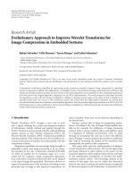
Fig. 1. System architecture.

3.1 Image Acquisition
The image database considered in this research work is composed by grayscale images,
acquired during a pavement surface visual survey over a Portuguese road. A digital camera
was manually positioned by the inspector with its optical axis perpendicular to the road
surface, at a distance of approximately 1.2 m. Images with different sizes are obtained
(2048×1536 pixels and 1858×1384 pixels), according to different camera setup procedures.
The digital camera is oriented in such a way that the images only contain areas belonging to
the road pavement surface. Moreover, the database includes images with several types of
cracks (longitudinal, transversal and miscellaneous), as well as images without any cracks.
Instead of processing the images at a pixel level in all the steps of the proposed system, each
image is divided into a set of non-overlapping regions of size 75×75 pixels. These
dimensions were empirically chosen, leading to a faster processing time and lower memory
storage requirements, while providing a good compromise between complexity and
accuracy. Database images can then be represented by smaller matrices, where each of their
values corresponds to the computation of region local statistics, as described next.


3.2 Selection of Training Images
Dealing with supervised classification strategies, training data (images for the envisaged
application) is necessary for classifiers learning. This section describes a technique for the
automatic selection of images, to be included in TIS, from the entire image database
acquired during the visual road pavement survey.
To allow a correct learning stage, training images should contain road pavement cracks.
Therefore, in a preliminary classification phase, all images are pre-processed in order to
detect the regions with most evident crack pixels, by exploiting the knowledge that regions

with crack pixels are supposed to have lower average intensities, when compared to regions
without crack pixels. The images are then sorted, starting from those where the longest
cracks were detected, the TIS being chosen from the top of this sorted list. The number of
images to be included in TIS is an option controlled by the system operator. Moreover, the
operator can edit the TIS, i.e., he can manually reject images automatically labeled by the
system as ‘training image’ or add additional ones. Images definitely labeled as ‘training
images’ are finally presented to the system operator, for manual identification of regions
containing crack pixels.
In this preliminary classification phase, image regions revealing evident crack pixels are
automatically labeled ‘1’, or ‘0’ otherwise. The result is a binary matrix (M
bm
) with
dimensions nl
bm
and nc
bm
, given by:



















r
img
bm
r
img
bm
nc
nc
fixnc
nl
nl
fixnl and

(1)
where nl
img
and nc
img
stand for the number of lines and columns of an image, respectively; nl
r

and nc
r
are the number of lines and columns of regions (here square regions of 75x75 are
used, as referred in Section 3.1), and fix is an operator which rounds a number towards zero.

Automatic image region labeling, in the preliminary classification phase, starts with the
computation of a regions’ mean values matrix - M
rm
, with dimensions nl
bm
× nc
bm
, each of its
elements representing the region’s pixel intensities average. This matrix is vertically and
horizontally scanned to find regions with evident crack pixels, by analyzing the variation of
the average region values when compared to those of the nearest neighbors, also taking into
account all the values along the line or column under analysis.
Starting with the vertical scanning of M
rm
, a region is considered a candidate of containing
cracks when the following logical decision, ld
(V)
, holds true:
 




0[2]Av[1]Av)mean(Bv )std(Bv )std(Av
j)(i,j)(i,j
2
j
1
j)(i,)(
 kkld

V

(2)
with
 
 




























0
Avstd
Avstd
0
Bv,
2
Av
)j,1(
)j,2(
j
)ji,(
)j,1i(),1i(
j)(i,
bm
nl
j
rm
rmrm

,
(3)

where rm
(i,j)
corresponds to the average pixel intensity of a region at position (i,j), k
1
and k

2

are parameters controlled by the system operator (set by default to an empirically chosen
value) and Av
(i,j)
and Bv
j
are column vectors with dimensions 2×1 and nlbm×1, respectively.
Elements of Bv
j
represent the standard deviation between region average intensities along
row i and column j (i.e. rm(i,j)) and the corresponding values of its nearest vertical
Supervised Crack Detection and Classication in Images of Road Pavement Flexible Surfaces 163

Training step
Select Training Images
Image Normalization & Saturation
Feature Extraction & Normalization
Parametric
Learning
Non-
parametric
Learning
Image Database
TIS TTIS
Decision
Boundary
Features
Evaluation
Ground Truth

Detection
Human
Labeling
Evaluation
Ground Truth
Classification
Crack Type Classification
Test step
Image Region
Labelling
(parametric)
Image Region
Labelling
(non-parametric)
Crack Detection

Fig. 1. System architecture.

3.1 Image Acquisition
The image database considered in this research work is composed by grayscale images,
acquired during a pavement surface visual survey over a Portuguese road. A digital camera
was manually positioned by the inspector with its optical axis perpendicular to the road
surface, at a distance of approximately 1.2 m. Images with different sizes are obtained
(2048×1536 pixels and 1858×1384 pixels), according to different camera setup procedures.
The digital camera is oriented in such a way that the images only contain areas belonging to
the road pavement surface. Moreover, the database includes images with several types of
cracks (longitudinal, transversal and miscellaneous), as well as images without any cracks.
Instead of processing the images at a pixel level in all the steps of the proposed system, each
image is divided into a set of non-overlapping regions of size 75×75 pixels. These
dimensions were empirically chosen, leading to a faster processing time and lower memory

storage requirements, while providing a good compromise between complexity and
accuracy. Database images can then be represented by smaller matrices, where each of their
values corresponds to the computation of region local statistics, as described next.


3.2 Selection of Training Images
Dealing with supervised classification strategies, training data (images for the envisaged
application) is necessary for classifiers learning. This section describes a technique for the
automatic selection of images, to be included in TIS, from the entire image database
acquired during the visual road pavement survey.
To allow a correct learning stage, training images should contain road pavement cracks.
Therefore, in a preliminary classification phase, all images are pre-processed in order to
detect the regions with most evident crack pixels, by exploiting the knowledge that regions
with crack pixels are supposed to have lower average intensities, when compared to regions
without crack pixels. The images are then sorted, starting from those where the longest
cracks were detected, the TIS being chosen from the top of this sorted list. The number of
images to be included in TIS is an option controlled by the system operator. Moreover, the
operator can edit the TIS, i.e., he can manually reject images automatically labeled by the
system as ‘training image’ or add additional ones. Images definitely labeled as ‘training
images’ are finally presented to the system operator, for manual identification of regions
containing crack pixels.
In this preliminary classification phase, image regions revealing evident crack pixels are
automatically labeled ‘1’, or ‘0’ otherwise. The result is a binary matrix (M
bm
) with
dimensions nl
bm
and nc
bm
, given by:



















r
img
bm
r
img
bm
nc
nc
fixnc
nl
nl
fixnl and

(1)
where nl
img
and nc
img
stand for the number of lines and columns of an image, respectively; nl
r

and nc
r
are the number of lines and columns of regions (here square regions of 75x75 are
used, as referred in Section 3.1), and fix is an operator which rounds a number towards zero.
Automatic image region labeling, in the preliminary classification phase, starts with the
computation of a regions’ mean values matrix - M
rm
, with dimensions nl
bm
× nc
bm
, each of its
elements representing the region’s pixel intensities average. This matrix is vertically and
horizontally scanned to find regions with evident crack pixels, by analyzing the variation of
the average region values when compared to those of the nearest neighbors, also taking into
account all the values along the line or column under analysis.
Starting with the vertical scanning of M
rm
, a region is considered a candidate of containing
cracks when the following logical decision, ld
(V)

, holds true:
 




0[2]Av[1]Av)mean(Bv )std(Bv )std(Av
j)(i,j)(i,j
2
j
1
j)(i,)(
 kkld
V

(2)
with
 
 




























0
Avstd
Avstd
0
Bv,
2
Av
)j,1(
)j,2(
j
)ji,(
)j,1i(),1i(
j)(i,
bm

nl
j
rm
rmrm

,
(3)

where rm
(i,j)
corresponds to the average pixel intensity of a region at position (i,j), k
1
and k
2

are parameters controlled by the system operator (set by default to an empirically chosen
value) and Av
(i,j)
and Bv
j
are column vectors with dimensions 2×1 and nlbm×1, respectively.
Elements of Bv
j
represent the standard deviation between region average intensities along
row i and column j (i.e. rm(i,j)) and the corresponding values of its nearest vertical
Recent Advances in Signal Processing164

neighboring regions ([rm
(i-1,j)
+ rm

(i+1,j)
]/2). Bv
j
is used to gather some knowledge about the
expected variations along the columns of M
rm
, highlighting the presence of relevant dark
pixels in regions, to be accounted for in equation (2). Regions with relevant crack pixels have
higher std(Bv
j
) values, due to higher Av
(i,j)
values when compared to regions without crack
pixels. Additionally, the values of Av
(1,j)
and
)j,(
Av
bm
nl
, i.e. the extreme regions of each
column (top and bottom edges), take value zero. After the vertical scanning of M
rm
, a binary
matrix, M
bm
(V)
, is build with the computed ld
(V)
values; it has the same dimensions of M

rm
.
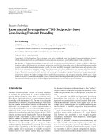
Fig. 2 is used to illustrate the behavior of std(Bv
j
) in the presence of cracks. It shows a
sample column of Mrm matrix (12
th
column) in two road pavement surface images. The
std(Bv
j
) value computed for the regions of the left image is lower (0.5696) than the
corresponding value for the right image (1.1895), due to the existence of an higher
std(Av
(11,12)
) value when compared to std(Av
(i,12)
) for the remaining regions. The same
tendency is observed for mean(Bv
j
), presenting a lower value for the left image (0.9405) than
for the right image (1.3788).


Fig. 2. Two sample images, with 1536x2048 pixels, from the pavement survey database. The
left image shows a pavement surface without cracks, while the right image includes a
transversal crack. Processed 75x75 pixel regions are marked with squares.

After the vertical scan, a horizontal scan proceeds in a similar way, acquainting for
longitudinal cracks, which would be difficult to detect in a vertical scan. Expressions (4) and
(5), for the horizontal scan, are similar to (2) and (3), with Av and Bv being replaced by Ah

and Bh, respectively:
 




0[2]Ah[1]Ah)mean(Bh )std(Bh )std(Ah
j)(i,j)(i,i
2
i
1
j)(i,)(
 kkld
H

(4)
   
 
0;Ahstd ;Ahstd;0Bh,;
2
Ah
)1(i,(i,2)i
),(
)1j(i,)1ji,(
j)(i, 











bm
nc
ji
rm
rmrm
,
(5)

with Ah
(i,j)
and Bh
i
being vectors with dimensions 2×1 and ncbm×1, respectively, and the
values for Ah
(i,1)
and
)(i,
Ah
bm
nc
, i.e. the extreme regions of each row (left and right edges),
taking value zero. After the horizontal scanning of M
rm
, a new binary matrix with the
computed ld

(H)
values is build, M
bm
(H)
(with the same dimensions of M
rm
).

(
11,12
)

(
11,12
)



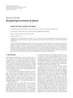
Fig. 3. Two sample images, with 1536x2048 pixels, from the pavement survey database. The
left image shows a pavement surface without cracks, while the right image includes a
longitudinal crack. Processed 75x75 pixel regions are marked with squares.

As an example, a horizontal scanning for the Mrm matrix 9th row of the images in Fig. 3 is
considered. Lower values for std(Bhi) and mean(Bhi) are obtain for the left image (0.6002
and 1.0681, respectively) than for the right image (0.9298 and 1.2171, respectively), due to
the existence of an higher std(Ah
(9,15)
) value when compared to std(Ah
(9,j)
) of the remaining

regions.
The next step of the preliminary detection of regions containing cracks is to merge the two
binary matrices M
bm
(V)
and M
bm
(H)
into a new binary matrix, M
bm
, to retain the results of both
the horizontal and vertical scans. The connected components of M
bm
are identified,
considering a 8-neighbourhood, and only those containing more than one region are kept as
crack region candidates; isolated crack region candidates are discarded (relabeled to ‘0’), as
they are likely to correspond to oil spots or other types of noise.
Finally, the length of each retained connect component is computed and, for each image, the
length of longest connected component (llcc) is stored. The selection of a given number of
training images (controlled by the system operator) is achieved by sorting the entire image
database in descending order of the computed llcc values – the TIS is chosen from the top of
this sorted list. This procedure ensures that the images selected for training the classifiers
effectively contain cracks.
Sample results of the binary matrices corresponding to images selected for the training step
are shown in Fig. 4, using k
1
and k
2
values equal to 0.4 and 2.0 respectively (empirically
chosen by the system operator). More detailed results and the corresponding analysis are

included in Section 6.1.
(
9,15
)

(
9,15
)

Supervised Crack Detection and Classication in Images of Road Pavement Flexible Surfaces 165

neighboring regions ([rm
(i-1,j)
+ rm
(i+1,j)
]/2). Bv
j
is used to gather some knowledge about the
expected variations along the columns of M
rm
, highlighting the presence of relevant dark
pixels in regions, to be accounted for in equation (2). Regions with relevant crack pixels have
higher std(Bv
j
) values, due to higher Av
(i,j)
values when compared to regions without crack
pixels. Additionally, the values of Av
(1,j)
and

)j,(
Av
bm
nl
, i.e. the extreme regions of each
column (top and bottom edges), take value zero. After the vertical scanning of M
rm
, a binary
matrix, M
bm
(V)
, is build with the computed ld
(V)
values; it has the same dimensions of M
rm
.
Fig. 2 is used to illustrate the behavior of std(Bv
j
) in the presence of cracks. It shows a
sample column of Mrm matrix (12
th
column) in two road pavement surface images. The
std(Bv
j
) value computed for the regions of the left image is lower (0.5696) than the
corresponding value for the right image (1.1895), due to the existence of an higher
std(Av
(11,12)
) value when compared to std(Av
(i,12)

) for the remaining regions. The same
tendency is observed for mean(Bv
j
), presenting a lower value for the left image (0.9405) than
for the right image (1.3788).


Fig. 2. Two sample images, with 1536x2048 pixels, from the pavement survey database. The
left image shows a pavement surface without cracks, while the right image includes a
transversal crack. Processed 75x75 pixel regions are marked with squares.

After the vertical scan, a horizontal scan proceeds in a similar way, acquainting for
longitudinal cracks, which would be difficult to detect in a vertical scan. Expressions (4) and
(5), for the horizontal scan, are similar to (2) and (3), with Av and Bv being replaced by Ah
and Bh, respectively:
 




0[2]Ah[1]Ah)mean(Bh )std(Bh )std(Ah
j)(i,j)(i,i
2
i
1
j)(i,)(
 kkld
H

(4)

   
 
0;Ahstd ;Ahstd;0Bh,;
2
Ah
)1(i,(i,2)i
),(
)1j(i,)1ji,(
j)(i, 










bm
nc
ji
rm
rmrm
,
(5)

with Ah
(i,j)
and Bh

i
being vectors with dimensions 2×1 and ncbm×1, respectively, and the
values for Ah
(i,1)
and
)(i,
Ah
bm
nc
, i.e. the extreme regions of each row (left and right edges),
taking value zero. After the horizontal scanning of M
rm
, a new binary matrix with the
computed ld
(H)
values is build, M
bm
(H)
(with the same dimensions of M
rm
).

(
11,12
)

(
11,12
)

Fig. 3. Two sample images, with 1536x2048 pixels, from the pavement survey database. The
left image shows a pavement surface without cracks, while the right image includes a
longitudinal crack. Processed 75x75 pixel regions are marked with squares.

As an example, a horizontal scanning for the Mrm matrix 9th row of the images in Fig. 3 is
considered. Lower values for std(Bhi) and mean(Bhi) are obtain for the left image (0.6002
and 1.0681, respectively) than for the right image (0.9298 and 1.2171, respectively), due to
the existence of an higher std(Ah
(9,15)
) value when compared to std(Ah
(9,j)
) of the remaining
regions.
The next step of the preliminary detection of regions containing cracks is to merge the two
binary matrices M
bm
(V)
and M
bm
(H)
into a new binary matrix, M
bm
, to retain the results of both
the horizontal and vertical scans. The connected components of M
bm
are identified,
considering a 8-neighbourhood, and only those containing more than one region are kept as
crack region candidates; isolated crack region candidates are discarded (relabeled to ‘0’), as

they are likely to correspond to oil spots or other types of noise.
Finally, the length of each retained connect component is computed and, for each image, the
length of longest connected component (llcc) is stored. The selection of a given number of
training images (controlled by the system operator) is achieved by sorting the entire image
database in descending order of the computed llcc values – the TIS is chosen from the top of
this sorted list. This procedure ensures that the images selected for training the classifiers
effectively contain cracks.
Sample results of the binary matrices corresponding to images selected for the training step
are shown in Fig. 4, using k
1
and k
2
values equal to 0.4 and 2.0 respectively (empirically
chosen by the system operator). More detailed results and the corresponding analysis are
included in Section 6.1.
(
9,15
)

(
9,15
)

Recent Advances in Signal Processing166

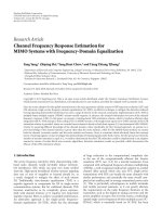
Fig. 4. Binary matrices showing the results of the preliminary crack region detection, for the
right images of Fig. 2 and Fig. 3, respectively. Regions in white are those preliminary
classified as containing relevant crack pixels.

3.3 Image Normalization and Saturation

As stated in Section 3.1, pavement surface images were acquired during a survey over a
Portuguese road using a digital camera. These images are free from shadows or other kind
of occlusions, caused for instance by trees near road footpaths, but they present a non-
uniform background illumination due to the type of sensor used, causing slight variations
on the regions’ pixel intensities average even in images without cracks.
To reduce this effect, an image normalization procedure is proposed. It consists in
computing a base intensity level value (bil
img
) for each image, equal to the average of the
elements of M
rm
corresponding to regions preliminary classified as not containing crack
pixels, i.e., those labeled with value ‘0’ in matrix M
bm
. The need to use M
bm
values for image
normalization is the reason why this step is performed after the selection of training images.
Based on the bil
img
value, a normalization constants matrix M
nc
(with the same dimension of
M
rm
) is computed for each image, its elements being real values lower or higher than 1.0.
The computation of M
nc
elements is different depending if the corresponding label in M
bm

is
’0’ or ‘1’.
For regions previously labeled with ‘0’, i.e. regions preliminary classified as not containing
cracks, the corresponding M
nc
elements are computed using the expression in (6):
 
 
'0'
'0'
ji,
ji,
rm
img
nc
M
bil
M 

(6)
where M
nc
(i,j)
’0’
stands for the normalization constant to be applied to region (i,j), which has
a M
bm
label ‘0’ and M
rm
(i,j)

’0’
is the corresponding element in M
rm
.
As an example, for a region with average pixel intensity of 163 and a M
nc
value of 0.92, all
that region’s original pixel values are affected by this normalization constant. The resulting
region average intensity will be 163×0.92=150.
For regions previously labelled with ‘1’, i.e. regions preliminary classified as containing
relevant cracks, the corresponding M
nc
elements are computed using the expression in (7):



 
 
 
 
 


a
ap
b
-bq
rm
img
nc

M
k
bil
M
'0'
0
'1'
qjp,i
1
ji,

(7)
where k
(0)
is the number of regions with label ‘0’ in a neighbourhood around the (i,j) region
under analysis and the double sum accounts for all the corresponding M
rm
elements. The
search for regions with label ‘0’ starts in 3×3 neighborhood (corresponding to a=b=1 in (7)).
A larger neighborhood is adopted (e.g., 5×5 which corresponds to a=b=2 in (7)) only if no
regions labeled ‘0’ are found in the previous one. For instance, a region with label ‘1’ and
average pixel intensity of 152, with four neighbors labeled ‘0’ and region averages of 148,
159, 140 and 153, has its original pixel intensities changed by a normalization constant of
152/150.
Expression (7) only considers regions with label ‘0’ for the computation of M
nc
(i,j)
’1’
. This is
done to prevent strong changes in pixel intensities of normalized regions with label ‘1’,

preventing dark pixels to become brighter than expected during the normalization step,
thus avoiding to loose the information that this region is likely to contain a crack.
Sample results using the proposed normalization procedure are shown in Fig. 5. The graph
on the left shows M
rm
original values, for the regions of the row considered in the right side
of Fig. 3; the graph on the right of Fig. 5 shows the normalized average intensity levels. As
can be seen from Fig. 5, the normalization procedure tends to equalize the average
intensities for those regions preliminary classified as not containing cracks, while
maintaining the average intensity of regions expected to contain crack pixels below bil
img
.


Fig. 5. Region average intensity values along the row selected in the right side of Fig. 3
before (left) and after (right) normalization.

Besides non-uniform background illumination, pavements surface images also frequently
reveal the presence of white pixels due to specular reflectance of some surface materials.
These pixels do not correspond to cracks but lead to higher intensity standard deviation
values, even for regions without cracks. Higher standard deviation of region intensities are
expected to be found in regions containing cracks (now due to higher differences between
dark crack pixels and the corresponding average computed for the entire region). Therefore,
white pixels may hinder detection performance, as different types of regions would present
similar local statistics.
Possible region
with crack pixels
Supervised Crack Detection and Classication in Images of Road Pavement Flexible Surfaces 167

Fig. 4. Binary matrices showing the results of the preliminary crack region detection, for the

right images of Fig. 2 and Fig. 3, respectively. Regions in white are those preliminary
classified as containing relevant crack pixels.

3.3 Image Normalization and Saturation
As stated in Section 3.1, pavement surface images were acquired during a survey over a
Portuguese road using a digital camera. These images are free from shadows or other kind
of occlusions, caused for instance by trees near road footpaths, but they present a non-
uniform background illumination due to the type of sensor used, causing slight variations
on the regions’ pixel intensities average even in images without cracks.
To reduce this effect, an image normalization procedure is proposed. It consists in
computing a base intensity level value (bil
img
) for each image, equal to the average of the
elements of M
rm
corresponding to regions preliminary classified as not containing crack
pixels, i.e., those labeled with value ‘0’ in matrix M
bm
. The need to use M
bm
values for image
normalization is the reason why this step is performed after the selection of training images.
Based on the bil
img
value, a normalization constants matrix M
nc
(with the same dimension of
M
rm
) is computed for each image, its elements being real values lower or higher than 1.0.

The computation of M
nc
elements is different depending if the corresponding label in M
bm
is
’0’ or ‘1’.
For regions previously labeled with ‘0’, i.e. regions preliminary classified as not containing
cracks, the corresponding M
nc
elements are computed using the expression in (6):
 
 
'0'
'0'
ji,
ji,
rm
img
nc
M
bil
M 

(6)
where M
nc
(i,j)
’0’
stands for the normalization constant to be applied to region (i,j), which has
a M

bm
label ‘0’ and M
rm
(i,j)
’0’
is the corresponding element in M
rm
.
As an example, for a region with average pixel intensity of 163 and a M
nc
value of 0.92, all
that region’s original pixel values are affected by this normalization constant. The resulting
region average intensity will be 163×0.92=150.
For regions previously labelled with ‘1’, i.e. regions preliminary classified as containing
relevant cracks, the corresponding M
nc
elements are computed using the expression in (7):



 
 
 
 
 


a
ap
b

-bq
rm
img
nc
M
k
bil
M
'0'
0
'1'
qjp,i
1
ji,

(7)
where k
(0)
is the number of regions with label ‘0’ in a neighbourhood around the (i,j) region
under analysis and the double sum accounts for all the corresponding M
rm
elements. The
search for regions with label ‘0’ starts in 3×3 neighborhood (corresponding to a=b=1 in (7)).
A larger neighborhood is adopted (e.g., 5×5 which corresponds to a=b=2 in (7)) only if no
regions labeled ‘0’ are found in the previous one. For instance, a region with label ‘1’ and
average pixel intensity of 152, with four neighbors labeled ‘0’ and region averages of 148,
159, 140 and 153, has its original pixel intensities changed by a normalization constant of
152/150.
Expression (7) only considers regions with label ‘0’ for the computation of M
nc

(i,j)
’1’
. This is
done to prevent strong changes in pixel intensities of normalized regions with label ‘1’,
preventing dark pixels to become brighter than expected during the normalization step,
thus avoiding to loose the information that this region is likely to contain a crack.
Sample results using the proposed normalization procedure are shown in Fig. 5. The graph
on the left shows M
rm
original values, for the regions of the row considered in the right side
of Fig. 3; the graph on the right of Fig. 5 shows the normalized average intensity levels. As
can be seen from Fig. 5, the normalization procedure tends to equalize the average
intensities for those regions preliminary classified as not containing cracks, while
maintaining the average intensity of regions expected to contain crack pixels below bil
img
.


Fig. 5. Region average intensity values along the row selected in the right side of Fig. 3
before (left) and after (right) normalization.

Besides non-uniform background illumination, pavements surface images also frequently
reveal the presence of white pixels due to specular reflectance of some surface materials.
These pixels do not correspond to cracks but lead to higher intensity standard deviation
values, even for regions without cracks. Higher standard deviation of region intensities are
expected to be found in regions containing cracks (now due to higher differences between
dark crack pixels and the corresponding average computed for the entire region). Therefore,
white pixels may hinder detection performance, as different types of regions would present
similar local statistics.
Possible region

with crack pixels
Recent Advances in Signal Processing168

In order to eliminate the undesired influence of white pixels, a region saturation algorithm
is proposed. For this purpose, the average of all pixel intensities of each normalized image is
computed (api) and all image pixels having intensities higher than api assume that value.
The pixel intensity saturation function is illustrated in Fig. 6. The effect of applying the pixel
intensity saturation algorithm to a normalized image is illustrated in Fig. 7.


Fig. 6. Pixel intensity saturation function.


Fig. 7. Normalized image containing a longitudinal crack before (left) and after (right)
applying the intensity saturation algorithm.

The proposed saturation function efficiently simplifies normalized images, reducing noise
and also the standard deviation of regions without crack pixels, while keeping all relevant
crack information.
To clarify the effect of applying the pixel saturation algorithm, which slightly changes the
regions’ average intensities, an example is shown in Fig. 8 for the row considered in the
right image of Fig. 3. At a first glance, comparing the right graph of Fig. 5 with the one on
top of Fig. 8, the region average intensities are globally lower for the second case. Moreover,
the corresponding standard deviations are also lower after applying the saturation
algorithm as seen in the bottom graphs of Fig. 8. In fact, the average standard deviation
value for the image regions preliminary classified as not containing cracks (26 out of the 27
regions in the example of Fig. 8) is 26.8, while after applying the saturation algorithm it is
reduced by approximately 54%, to 12.4. Still, for the region likely to contain cracks, the
reduction is only 29% (31.5 against 44.1 in the non-saturated case).
Thus, the saturation algorithm achieves a strong standard deviation reduction for regions

without cracks, creating a good separation to the standard deviation values of crack regions,
api

Original pixel

intensit
y
values

Saturated pixel

intensit
y
values

api


and allowing to consider it, together with the region average intensities, as the features to be
exploited by the classifier used for crack regions detection, as discussed in the next section.



Fig. 8. Region average intensity values along the row selected in the right side of Fig. 3 after
normalization and saturation (top) and standard deviation of region intensities for the
normalized images before (bottom left) and after applying the saturation algorithm (bottom
right).

3.4 Feature Extraction and Normalization
To automatically label regions as containing cracks or not, a pattern recognition system

operating over a simple feature space is proposed. The feature space is two dimensional,
being constructed using regions’ local statistics, computed for normalized and saturated
images. The first feature is the mean value of all pixel intensities in a region; the second is
the standard deviation of the region’s pixel intensities. Images can then be represented in
the feature space - see example in Fig. 9, where each point identifies a region of an image.
Since different images present different average values, as can be observed by the scattering
of points in Fig. 9 top-right and bottom-left images, a further normalization step is needed to
allow a better classifier performance.
This additional feature space normalization starts with the computation of each image’s two
dimensional feature space centroid, together with a global centroid computed for all the
Region preliminary
classified as containing
crack pixels
Amplitude
Amplitude
26.8
12.4

44.1
31.5
Supervised Crack Detection and Classication in Images of Road Pavement Flexible Surfaces 169

In order to eliminate the undesired influence of white pixels, a region saturation algorithm
is proposed. For this purpose, the average of all pixel intensities of each normalized image is
computed (api) and all image pixels having intensities higher than api assume that value.
The pixel intensity saturation function is illustrated in Fig. 6. The effect of applying the pixel
intensity saturation algorithm to a normalized image is illustrated in Fig. 7.


Fig. 6. Pixel intensity saturation function.

Fig. 7. Normalized image containing a longitudinal crack before (left) and after (right)
applying the intensity saturation algorithm.

The proposed saturation function efficiently simplifies normalized images, reducing noise
and also the standard deviation of regions without crack pixels, while keeping all relevant
crack information.
To clarify the effect of applying the pixel saturation algorithm, which slightly changes the
regions’ average intensities, an example is shown in Fig. 8 for the row considered in the
right image of Fig. 3. At a first glance, comparing the right graph of Fig. 5 with the one on
top of Fig. 8, the region average intensities are globally lower for the second case. Moreover,
the corresponding standard deviations are also lower after applying the saturation
algorithm as seen in the bottom graphs of Fig. 8. In fact, the average standard deviation
value for the image regions preliminary classified as not containing cracks (26 out of the 27
regions in the example of Fig. 8) is 26.8, while after applying the saturation algorithm it is
reduced by approximately 54%, to 12.4. Still, for the region likely to contain cracks, the
reduction is only 29% (31.5 against 44.1 in the non-saturated case).
Thus, the saturation algorithm achieves a strong standard deviation reduction for regions
without cracks, creating a good separation to the standard deviation values of crack regions,
api

Original pixel

intensit
y
values

Saturated pixel

intensit
y
values

api


and allowing to consider it, together with the region average intensities, as the features to be
exploited by the classifier used for crack regions detection, as discussed in the next section.



Fig. 8. Region average intensity values along the row selected in the right side of Fig. 3 after
normalization and saturation (top) and standard deviation of region intensities for the
normalized images before (bottom left) and after applying the saturation algorithm (bottom
right).

3.4 Feature Extraction and Normalization
To automatically label regions as containing cracks or not, a pattern recognition system
operating over a simple feature space is proposed. The feature space is two dimensional,
being constructed using regions’ local statistics, computed for normalized and saturated
images. The first feature is the mean value of all pixel intensities in a region; the second is
the standard deviation of the region’s pixel intensities. Images can then be represented in
the feature space - see example in Fig. 9, where each point identifies a region of an image.
Since different images present different average values, as can be observed by the scattering
of points in Fig. 9 top-right and bottom-left images, a further normalization step is needed to
allow a better classifier performance.
This additional feature space normalization starts with the computation of each image’s two
dimensional feature space centroid, together with a global centroid computed for all the
Region preliminary

classified as containing
crack pixels
Amplitude
Amplitude
26.8
12.4

44.1
31.5
Recent Advances in Signal Processing170

database images. Then, for each individual image, the two dimensional feature space points
are translated to align the respective centroid with the global one. The corresponding result
is illustrated in the bottom-right image of Fig. 9. Table 1 complements these results with the
values of the intraclass and interclass distances (Heijden et al., 2004), computed for a TIS
image set composed of five images, as discussed in Section 6.



Fig. 9. Feature space representation, using a TIS composed of five images, for the original
image (top-left), after image normalization (top-right), after normalization and saturation
(bottom-left) and after the additional feature space normalization (bottom-right).

Implementations

Intraclass
distance
(crack
regions)
Intraclass

distance



(no crack
regions)
Interclass

distance
Crack
region’s
intra/
interclass
ratio
(%)
No crack
region’s
intra/interclas
s ratio (%)
Original
images
147.9 145.0 395.8 37.4 36.6
Norm. 150.4 59.1 371.4 40.5 15.9
Norm. + Satur. 138.7 45.5 423.9 32.7 10.7
Norm. + Satur.
+ Trans.
87.2 8.7 402.4 21.7 2.2
Table 1: Interclass and intraclass distances computed using TIS set.

As can be seen in the first line of Table 1, high intraclass and interclass distance values are

obtained for the original images, denoting a very scattered feature space where class
separation would be a difficult task, as illustrated by the top-right graph of Fig. 9.
After region normalization (top-right graph of Fig. 9), non crack regions points become
aligned along vertical lines (each vertical alignment corresponding to an image), with very
little variation along the horizontal axis. For these points, the values of the second line of
Table 1 show a better class compactness. The distribution of crack region’s points is not
significantly affected by this task.
Applying the saturation algorithm to the normalized images (see bottom-left graph in Fig. 9)
a reduction of the intraclass to interclass distance ratio is obtained for both classes.
With feature space normalization a further improvement is observed in the results. The
intraclass to interclass distance ratios is the best (21.7% and 2.2%), revealing a more
separable feature space and more compact point distributions.

4. Training and Classification

This section describes the classification strategies being evaluated, which are based on two
supervised learning approaches: parametric (Section 4.1) and nonparametric (Section 4.2).
Parametric approaches are based on a bivariate class-conditional normal density, as it
provides a good data description (Oliveira & Correia, 2007).

4.1 Parametric Learning and Classification
Points obtained by applying the described feature extraction and normalization procedures
to the training image set (TIS) are manually labeled by a skilled system operator, providing
a training data set for which the labels are a priori known.
From a fully automatic application point-of-view this is a drawback, as a human operator is
required to manually label image regions. However, since the aim here is to develop
parametric supervised strategies for crack region detection, the manual labeling is required
to create the training data to be used by the classifiers’ parameter learning step.
All TIS feature points compose a pattern vector x, representing a sample of the random
variable X, taking values on a sample space X. For each element x

i
of pattern vector x, one
possible class y
i
is assigned, where Y is the class set, .i.e. y
i
Y. Thus, the training set is:








21
2
11
,;:,, ccyxyxyx
iinn
 

(8)
where n is the number of points of the pattern vector x. Only two classes are used: regions
with crack pixels, labeled as class c
1
, and regions without crack pixels, labeled as class c
2
.
Assigning a loss penalty to misclassified measurements, the minimal expectation of the

resulting cost is taken as an acceptable optimization criterion for the Bayesian classifier
presented here (Heijden et al., 2004):






iii
ypypy |xln maxarg
ˆ
i
y


(9)
where p(y
i
) are the class priors, computed by:
 
classes all for points of number total

k
ki
c
cyp
class into labeled points #

.
(10)

Supervised Crack Detection and Classication in Images of Road Pavement Flexible Surfaces 171

database images. Then, for each individual image, the two dimensional feature space points
are translated to align the respective centroid with the global one. The corresponding result
is illustrated in the bottom-right image of Fig. 9. Table 1 complements these results with the
values of the intraclass and interclass distances (Heijden et al., 2004), computed for a TIS
image set composed of five images, as discussed in Section 6.



Fig. 9. Feature space representation, using a TIS composed of five images, for the original
image (top-left), after image normalization (top-right), after normalization and saturation
(bottom-left) and after the additional feature space normalization (bottom-right).

Implementations

Intraclass
distance
(crack
regions)
Intraclass
distance



(no crack
regions)
Interclass

distance
Crack
region’s
intra/
interclass
ratio
(%)
No crack
region’s
intra/interclas
s ratio (%)
Original
images
147.9 145.0 395.8 37.4 36.6
Norm. 150.4 59.1 371.4 40.5 15.9
Norm. + Satur. 138.7 45.5 423.9 32.7 10.7
Norm. + Satur.
+ Trans.
87.2 8.7 402.4 21.7 2.2
Table 1: Interclass and intraclass distances computed using TIS set.

As can be seen in the first line of Table 1, high intraclass and interclass distance values are
obtained for the original images, denoting a very scattered feature space where class
separation would be a difficult task, as illustrated by the top-right graph of Fig. 9.
After region normalization (top-right graph of Fig. 9), non crack regions points become
aligned along vertical lines (each vertical alignment corresponding to an image), with very
little variation along the horizontal axis. For these points, the values of the second line of
Table 1 show a better class compactness. The distribution of crack region’s points is not
significantly affected by this task.

Applying the saturation algorithm to the normalized images (see bottom-left graph in Fig. 9)
a reduction of the intraclass to interclass distance ratio is obtained for both classes.
With feature space normalization a further improvement is observed in the results. The
intraclass to interclass distance ratios is the best (21.7% and 2.2%), revealing a more
separable feature space and more compact point distributions.

4. Training and Classification

This section describes the classification strategies being evaluated, which are based on two
supervised learning approaches: parametric (Section 4.1) and nonparametric (Section 4.2).
Parametric approaches are based on a bivariate class-conditional normal density, as it
provides a good data description (Oliveira & Correia, 2007).

4.1 Parametric Learning and Classification
Points obtained by applying the described feature extraction and normalization procedures
to the training image set (TIS) are manually labeled by a skilled system operator, providing
a training data set for which the labels are a priori known.
From a fully automatic application point-of-view this is a drawback, as a human operator is
required to manually label image regions. However, since the aim here is to develop
parametric supervised strategies for crack region detection, the manual labeling is required
to create the training data to be used by the classifiers’ parameter learning step.
All TIS feature points compose a pattern vector x, representing a sample of the random
variable X, taking values on a sample space X. For each element x
i
of pattern vector x, one
possible class y
i
is assigned, where Y is the class set, .i.e. y
i
Y. Thus, the training set is:









21
2
11
,;:,, ccyxyxyx
iinn
 

(8)
where n is the number of points of the pattern vector x. Only two classes are used: regions
with crack pixels, labeled as class c
1
, and regions without crack pixels, labeled as class c
2
.
Assigning a loss penalty to misclassified measurements, the minimal expectation of the
resulting cost is taken as an acceptable optimization criterion for the Bayesian classifier
presented here (Heijden et al., 2004):







iii
ypypy |xln maxarg
ˆ
i
y


(9)
where p(y
i
) are the class priors, computed by:
 
classes all for points of number total

k
ki
c
cyp
class into labeled points #

.
(10)


Recent Advances in Signal Processing172

with k being the class index. A loss function L(s,a) : S×A → R is constructed to quantify the
cost of each classification action, where S is the state space, s is the true state of nature, A is
the action space and a is the action (classification) taken by the classifier (Figueiredo, 2004).

The decision rule is to take the action that minimizes the associated risk, i.e., take action a
1
if
R(a
1
|x) is lower than R(a
2
|x), where a
k
means classifying measurement x
i
into class c
k
with
k{1,2}, symbolically represented by (Duda et al., 2004):
       
22
1121
2212
2
1
11
|
LL
LL
| cyPcyp
c
c
cyPcyp
iiii














 xx

(11)
where L
pq
is the loss resulting from classifying a measurement into class c
p
, while the true
state of nature is class c
q
, i.e.


qipi
c
y
c

y


|
ˆ
L
. Since a uniform loss function is used here,
i.e. L
11
= L
22
=1 and L
12
= L
21
=0, the expression in (10) identifies a maximum a posteriori
probability classifier. Ground truth for the training set is known, thus the parameters for
both classes are learned from TIS feature points, X~N(

k
,
k
), with (Bishop, 2006):



k
n
i
i

k
k
k
x
n
1
1
ˆ

and
  
T
1
ˆˆ
1
1
ˆ
k
i
k
n
i
k
i
k
k
k
xx
n
k








(12)
where
k

ˆ
is the sample unbiased vector mean,
k

ˆ
is the sample unbiased covariance matrix,
k is the class index and n
k
is the total number of k class points.
Three ways to compute the decision boundaries are considered. The first one, denoted as
linear, assumes a joint sample covariance matrix (), with the boundary being computed by
a weighted average (according to the class prior probabilities) of each class’ covariance
matrix, which results in a linear decision boundary (Duda et al., 2004; Heijden et al., 2004)
given by:
0
T


x

(13)

1
1T
12
1T
2
1
2
)(
)(
ln2






cyP
cyP
i
i

(14)

 
12
1
2





(15)
The second way to compute the decision boundary, denoted as quadratic, assumes a general
covariance matrix resulting in the quadratic boundary (Heijden et al., 2004) defined by:
0
TT
 xxx


(16)

1
1
1
T
12
1
2
T
2
1
2
21
)(
)(
ln2lnln







cyP
c
y
P
i
i

(17)



1
1
12
1
2
2



and
1
1
1
2




(18)





The third decision boundary, denoted as independent, is computed assuming independent
features, i.e. the covariance matrices in (12) are now diagonal matrices computed as:






llllll
kkkkk

 xxE
ˆ
,

(19)
and
ml
k
,
ˆ


takes value zero whenever l ≠ m; E stands for the expected value and l and m are
feature identifiers, taking value 1 or 2 for class regions without or with crack pixels,
respectively. Using these new covariance matrices, equations from (16) to (18) are used to
compute the target decision boundary.
A sample result using the three types of decision boundaries, computed for the TIS, is
illustrated in Fig. 10.


Fig. 10. Three parametric decision boundaries computed for the TIS.

4.2 Non-parametric Learning and Classification
This subsection deals with classifiers that operate when both conditional probability
distributions are unavailable. This is different from the parametric case, where the only
unknowns were the probability density parameters modeling the data.
In general, one advantage of non-parametric learning, when compared with parametric
learning, is that not so much prior knowledge about the data to be processed is required,
but, on the other hand, a large amount of data is needed to compensate the lack of
knowledge about probability density functions, although it can be reduced when certain
computational constrains of the classifiers apply (for example, the use of a linear boundary
decision instead of a non-linear one) and they match the inherent distributions (Heihjen et
al., 2004; Webb, 2002).
Here, three non-parametric techniques are considered: Parzen windows, k-Nearest
Neighbor and Fisher's Least Square Linear classifiers.

Supervised Crack Detection and Classication in Images of Road Pavement Flexible Surfaces 173

with k being the class index. A loss function L(s,a) : S×A → R is constructed to quantify the
cost of each classification action, where S is the state space, s is the true state of nature, A is
the action space and a is the action (classification) taken by the classifier (Figueiredo, 2004).
The decision rule is to take the action that minimizes the associated risk, i.e., take action a
1
if
R(a
1
|x) is lower than R(a
2
|x), where a
k
means classifying measurement x
i
into class c
k
with
k{1,2}, symbolically represented by (Duda et al., 2004):
       
22
1121
2212
2
1
11
|
LL
LL

| cyPcyp
c
c
cyPcyp
iiii













 xx

(11)
where L
pq
is the loss resulting from classifying a measurement into class c
p
, while the true
state of nature is class c
q
, i.e.



qipi
c
y
c
y


|
ˆ
L
. Since a uniform loss function is used here,
i.e. L
11
= L
22
=1 and L
12
= L
21
=0, the expression in (10) identifies a maximum a posteriori
probability classifier. Ground truth for the training set is known, thus the parameters for
both classes are learned from TIS feature points, X~N(

k
,
k
), with (Bishop, 2006):




k
n
i
i
k
k
k
x
n
1
1
ˆ

and
  
T
1
ˆˆ
1
1
ˆ
k
i
k
n
i
k
i
k

k
k
xx
n
k







(12)
where
k

ˆ
is the sample unbiased vector mean,
k

ˆ
is the sample unbiased covariance matrix,
k is the class index and n
k
is the total number of k class points.
Three ways to compute the decision boundaries are considered. The first one, denoted as
linear, assumes a joint sample covariance matrix (), with the boundary being computed by
a weighted average (according to the class prior probabilities) of each class’ covariance
matrix, which results in a linear decision boundary (Duda et al., 2004; Heijden et al., 2004)
given by:

0
T


x

(13)

1
1T
12
1T
2
1
2
)(
)(
ln2






cyP
cyP
i
i

(14)

 
12
1
2




(15)
The second way to compute the decision boundary, denoted as quadratic, assumes a general
covariance matrix resulting in the quadratic boundary (Heijden et al., 2004) defined by:
0
TT
 xxx


(16)

1
1
1
T
12
1
2
T
2
1
2

21
)(
)(
ln2lnln






cyP
c
y
P
i
i

(17)



1
1
12
1
2
2




and
1
1
1
2



(18)





The third decision boundary, denoted as independent, is computed assuming independent
features, i.e. the covariance matrices in (12) are now diagonal matrices computed as:






llllll
kkkkk

 xxE
ˆ
,

(19)

and
ml
k
,
ˆ

takes value zero whenever l ≠ m; E stands for the expected value and l and m are
feature identifiers, taking value 1 or 2 for class regions without or with crack pixels,
respectively. Using these new covariance matrices, equations from (16) to (18) are used to
compute the target decision boundary.
A sample result using the three types of decision boundaries, computed for the TIS, is
illustrated in Fig. 10.


Fig. 10. Three parametric decision boundaries computed for the TIS.

4.2 Non-parametric Learning and Classification
This subsection deals with classifiers that operate when both conditional probability
distributions are unavailable. This is different from the parametric case, where the only
unknowns were the probability density parameters modeling the data.
In general, one advantage of non-parametric learning, when compared with parametric
learning, is that not so much prior knowledge about the data to be processed is required,
but, on the other hand, a large amount of data is needed to compensate the lack of
knowledge about probability density functions, although it can be reduced when certain
computational constrains of the classifiers apply (for example, the use of a linear boundary
decision instead of a non-linear one) and they match the inherent distributions (Heihjen et
al., 2004; Webb, 2002).
Here, three non-parametric techniques are considered: Parzen windows, k-Nearest
Neighbor and Fisher's Least Square Linear classifiers.

Recent Advances in Signal Processing174

The implemented Parzen algorithm for learning and classification follows the descriptions
in (Heijden et al., 2004). Considering a labeled training vector x according to (8) and an
unlabelled test set, the probability density estimation for an arbitrary test vector z is
achieved by:
 
















k
n

q
k
ki
fsfsn
cyp
1
2
2
2
exp
2
11
|
ˆ
  
A
2
xz
z
q


(20)
where
A is a kernel that represents the knowledge about the distance between a test
measurement
z and the training measurement x
q
, corresponding to a Gaussian interpolation
distance function, n

k
is the total number of measurements for class k and fs is a constant that
controls the size of the kernel influence zone, computed such that it maximizes:
  

 

2
1 1
|
ˆ
ln
k
n
q
kik,q
k
cyp x

(21)
where x
k,q
is the sample q of the class k which is left out by the leave-one-out method when
computing the estimation of the posterior probability density. A measurement is classified
into class c
k
with the maximum posterior probability:
   



kiki
k
cyPcypk 

ˆ
ˆ
argmax
ˆ
2,1
|z

(22)
where
 
ki
cyP 
ˆ
represents class priors according to (10).
For
k-Nearest Neighbors classification (k-nn), the estimated posterior probability density may
have different resolutions when the training data is not homogeneous, i.e., it’s resolution is
higher when the training data is more dense. The posterior probability density for an arbitrary
test vector
z is computed by (Duda et al., 2001; Theodoridis & Foutroumbas, 2003):
 
 
z
z
V
k

k
ki
n
N
cyp |
ˆ

(23)
where N
k
is the number of samples inside the volume V(z)—which represents a sphere
centered in
z—belonging to class k and n
k
is the total number of training samples belonging
to class k. Thus, a measurement is classified into the class (c
1
or c
2
) that contains more
training measurements in the N
k
neighborhood of z:
   




k
k

kiki
k
NcyPcypk
2,12,1
maxarg
ˆ
|
ˆ
maxarg
ˆ

 z

(24)
where
 
ki
cyP 
ˆ
again represents the class priors according to (10).
The aim of the
Fischer’s linear classification strategy is to find the linear discriminant
function between both classes, which corresponds to the projection that maximizes the class
separability (Bishop, 2006; Duda et. al., 2001). Class separability in a direction d
n

is
defined by:
dJd
dJd

dR
W
T
B
T
)(

(25)
which is also denoted as the ratio of the between-class covariance matrix (J
B
) to the within-
class covariance matrix (J
K
), defined as:




T
B
J
2121



(26)

21
cc
WWW

JJJ 
,



2
1
))
k
T
kkkkW
k
c
J

xx

(27)
where

k
denotes the vector mean for class k, computed according to (12) and x
k
is class k
measurements vector data. An estimate of d is obtained maximizing (25) according to:










dJd
dJd
d
W
T
B
T
d
argmax
ˆ

(28)
Thus, a measurement from a vector
z is classified into class c
1
when y(x
i
)≥y
0
for y
0
=Kz (z is
classified into class c
2
otherwise).
A sample result using the three types of decision boundaries, computed using the TIS, is

illustrated in Fig.
11.


Fig. 11. Three non-parametric decision boundaries computed for the TIS. For k-nn, the
boundary shown corresponds to a neighborhood of 1 point.

5. Crack Type Classification

Detection results are stored in binary matrices (one for each TTIS image) with the same
dimensions as (1), where ‘1’ means regions labeled as containing crack pixels and ‘0’ the
opposite case. All binary matrices are then processed to identify connect components and
the resulting connected crack regions are finally classified into one of the crack types
considered in the scope of this research work, following the specifications of the Portuguese
Distress Catalog (JAE, 1997): longitudinal (c
L
), transversal (c
T
) or miscellaneous (c
M
).
Crack type classification uses another pattern classification system exploiting a new 2D
feature space. A crack type label is assigned to each connected crack region and
cumulatively added to each TTIS image.
The 2D feature space used for crack type classification is composed by the standard
deviations of the column (feature one) and row (feature two) coordinates of connected crack
regions. A sample representation of this feature space is given in Fig.
12.

Supervised Crack Detection and Classication in Images of Road Pavement Flexible Surfaces 175

The implemented Parzen algorithm for learning and classification follows the descriptions
in (Heijden et al., 2004). Considering a labeled training vector x according to (8) and an
unlabelled test set, the probability density estimation for an arbitrary test vector z is
achieved by:
 
















k
n
q
k
ki
fsfsn
cyp
1

2
2
2
exp
2
11
|
ˆ
  
A
2
xz
z
q


(20)
where
A is a kernel that represents the knowledge about the distance between a test
measurement
z and the training measurement x
q
, corresponding to a Gaussian interpolation
distance function, n
k
is the total number of measurements for class k and fs is a constant that
controls the size of the kernel influence zone, computed such that it maximizes:
  

 


2
1 1
|
ˆ
ln
k
n
q
kik,q
k
cyp x

(21)
where x
k,q
is the sample q of the class k which is left out by the leave-one-out method when
computing the estimation of the posterior probability density. A measurement is classified
into class c
k
with the maximum posterior probability:
   


kiki
k
cyPcypk 

ˆ
ˆ

argmax
ˆ
2,1
|z

(22)
where
 
ki
cyP 
ˆ
represents class priors according to (10).
For
k-Nearest Neighbors classification (k-nn), the estimated posterior probability density may
have different resolutions when the training data is not homogeneous, i.e., it’s resolution is
higher when the training data is more dense. The posterior probability density for an arbitrary
test vector
z is computed by (Duda et al., 2001; Theodoridis & Foutroumbas, 2003):
 
 
z
z
V
k
k
ki
n
N
cyp |
ˆ

(23)
where N
k
is the number of samples inside the volume V(z)—which represents a sphere
centered in
z—belonging to class k and n
k
is the total number of training samples belonging
to class k. Thus, a measurement is classified into the class (c
1
or c
2
) that contains more
training measurements in the N
k
neighborhood of z:
   




k
k
kiki
k
NcyPcypk
2,12,1
maxarg
ˆ

|
ˆ
maxarg
ˆ

 z

(24)
where
 
ki
cyP 
ˆ
again represents the class priors according to (10).
The aim of the
Fischer’s linear classification strategy is to find the linear discriminant
function between both classes, which corresponds to the projection that maximizes the class
separability (Bishop, 2006; Duda et. al., 2001). Class separability in a direction d
n

is
defined by:
dJd
dJd
dR
W
T
B
T
)(

(25)
which is also denoted as the ratio of the between-class covariance matrix (J
B
) to the within-
class covariance matrix (J
K
), defined as:




T
B
J
2121



(26)

21
cc
WWW
JJJ 
,



2

1
))
k
T
kkkkW
k
c
J

xx

(27)
where

k
denotes the vector mean for class k, computed according to (12) and x
k
is class k
measurements vector data. An estimate of d is obtained maximizing (25) according to:









dJd
dJd

d
W
T
B
T
d
argmax
ˆ

(28)
Thus, a measurement from a vector
z is classified into class c
1
when y(x
i
)≥y
0
for y
0
=Kz (z is
classified into class c
2
otherwise).
A sample result using the three types of decision boundaries, computed using the TIS, is
illustrated in Fig.
11.


Fig. 11. Three non-parametric decision boundaries computed for the TIS. For k-nn, the
boundary shown corresponds to a neighborhood of 1 point.

5. Crack Type Classification

Detection results are stored in binary matrices (one for each TTIS image) with the same
dimensions as (1), where ‘1’ means regions labeled as containing crack pixels and ‘0’ the
opposite case. All binary matrices are then processed to identify connect components and
the resulting connected crack regions are finally classified into one of the crack types
considered in the scope of this research work, following the specifications of the Portuguese
Distress Catalog (JAE, 1997): longitudinal (c
L
), transversal (c
T
) or miscellaneous (c
M
).
Crack type classification uses another pattern classification system exploiting a new 2D
feature space. A crack type label is assigned to each connected crack region and
cumulatively added to each TTIS image.
The 2D feature space used for crack type classification is composed by the standard
deviations of the column (feature one) and row (feature two) coordinates of connected crack
regions. A sample representation of this feature space is given in Fig.
12.

Recent Advances in Signal Processing176


Fig. 12. 2D feature space used for crack type classification. Point L
1
represents a connected
crack region classified as a ‘longitudinal crack’.

The bisectrix sectioning the 2D feature space into two zones, ‘Z1’ and ‘Z2’, represents the
points where connected components have equal column and row standard deviation values,
identifying perfect miscellaneous cracks. Points positioned over the horizontal or vertical
axes correspond to perfect transversal or longitudinal cracks, respectively.
Crack type classification is performed by computing two distances for each connected crack
region point representation in the 2D feature space: d
L
and d
A
, where d
L
is the distance from
the point to the bisectrix axis and d
A
corresponds to the distance to nearest axis (horizontal
or vertical). The example in Fig.
12 shows the classification of one connected crack region
(point L
1
) as a ‘longitudinal crack’ (d
L
> d
A
). This crack type classification is fully automatic
and unsupervised, no training stage being required.
The probability of a crack belonging to class c
L
or c
T

is computed, according to:
 
ii
i
icri
rcyP
LA
A
dd
d
1|



(29)

while the probability of a crack belonging to the miscellaneous cracks class (c
M
) is computed
according to:
 
ii
i
iMi
rcyP
LA
L
dd
d
1|




(30)
where the index
cr
is one of the class indexes T or L, d
Ai
is the distance from point i to the
nearest axis, d
Li
is the distance from point i to the bisectrix and r
i
is the observation (region i).
Thus, a connected crack region is classified into the class presenting a probability above 0.5:

a crack is classified as ‘longitudinal’ (class c
L
) if d
L
> d
A
and the nearest axis is the
vertical one;

a crack is classified as ‘transversal’ (class c
T
) if d
L
> d

A
and the nearest axis is the
horizontal one;

a crack is classified as ‘miscellaneous’ (class c
M
) if d
A
> d
L
, independently of the
nearest axis.





6. Experimental Results and Performance Evaluation

The proposed classification strategies are evaluated over the TTIS, which is composed by
real flexible pavement surface images, eventually containing cracks with linear
development. These images were acquired during a survey over a Portuguese road and
ground truth data has been manually constructed. Part of the algorithmic development was
supported by the PRtools toolbox (Duin et al., 2004). Experimental results are firstly
presented for crack regions detection (Section 6.1) and then for crack type classification
(Section 6.2).

6.1 Crack Regions Detection Results and Evaluation
Sample results for one TTIS image using the available classifiers are shown in Fig. 13. For
the k-nn strategy, one nearest neighbor (1-nn) is considered, as this is the neighborhood that

optimizes the leave-one-out error for the target image.
An evaluation of the different strategies, by comparison with the ground truth data, is
included in Table 2. A global Error-rate is computed (e-r
G
being the classification error for
classes c
1
and c
2
), as well as some metrics related only to regions with crack pixels: Crack
Error-rate (e-r
Cr
), Precision (pr), Recall (re) as well as a Performance Criterion (pc) reflecting
the overall classifier performance, according to (Tax, 2006):

regions of number Total

and


classes

for

classified

wron
g
l
y

re
g
ions

o
f

Number
21
cc
re
G


(31)
re
c
re
Cr
 1
truth) (ground regionscrack of number Total

class

for

classified

wrongly

regions

o
f

Number
1

(32)
detected regionscrack of number Total

class

for

classified

correctl
y

re
g
ions

of

Number
1
c

pr 

(33)
truth) (ground regionscrack of number Total

class

for

classified

correctl
y

re
g
ions

o
f

Number
1
c
re 

(34)
repr
re
p

r
pc




2
.
(35)
Supervised Crack Detection and Classication in Images of Road Pavement Flexible Surfaces 177


Fig. 12. 2D feature space used for crack type classification. Point L
1
represents a connected
crack region classified as a ‘longitudinal crack’.

The bisectrix sectioning the 2D feature space into two zones, ‘Z1’ and ‘Z2’, represents the
points where connected components have equal column and row standard deviation values,
identifying perfect miscellaneous cracks. Points positioned over the horizontal or vertical
axes correspond to perfect transversal or longitudinal cracks, respectively.
Crack type classification is performed by computing two distances for each connected crack
region point representation in the 2D feature space: d
L
and d
A
, where d
L
is the distance from
the point to the bisectrix axis and d

A
corresponds to the distance to nearest axis (horizontal
or vertical). The example in Fig.
12 shows the classification of one connected crack region
(point L
1
) as a ‘longitudinal crack’ (d
L
> d
A
). This crack type classification is fully automatic
and unsupervised, no training stage being required.
The probability of a crack belonging to class c
L
or c
T
is computed, according to:
 
ii
i
icri
rcyP
LA
A
dd
d
1|



(29)

while the probability of a crack belonging to the miscellaneous cracks class (c
M
) is computed
according to:
 
ii
i
iMi
rcyP
LA
L
dd
d
1|



(30)
where the index
cr
is one of the class indexes T or L, d
Ai
is the distance from point i to the
nearest axis, d
Li
is the distance from point i to the bisectrix and r
i
is the observation (region i).

Thus, a connected crack region is classified into the class presenting a probability above 0.5:

a crack is classified as ‘longitudinal’ (class c
L
) if d
L
> d
A
and the nearest axis is the
vertical one;

a crack is classified as ‘transversal’ (class c
T
) if d
L
> d
A
and the nearest axis is the
horizontal one;

a crack is classified as ‘miscellaneous’ (class c
M
) if d
A
> d
L
, independently of the
nearest axis.

6. Experimental Results and Performance Evaluation

The proposed classification strategies are evaluated over the TTIS, which is composed by
real flexible pavement surface images, eventually containing cracks with linear
development. These images were acquired during a survey over a Portuguese road and
ground truth data has been manually constructed. Part of the algorithmic development was
supported by the PRtools toolbox (Duin et al., 2004). Experimental results are firstly
presented for crack regions detection (Section 6.1) and then for crack type classification
(Section 6.2).

6.1 Crack Regions Detection Results and Evaluation
Sample results for one TTIS image using the available classifiers are shown in Fig. 13. For
the k-nn strategy, one nearest neighbor (1-nn) is considered, as this is the neighborhood that
optimizes the leave-one-out error for the target image.
An evaluation of the different strategies, by comparison with the ground truth data, is
included in Table 2. A global Error-rate is computed (e-r
G
being the classification error for
classes c
1
and c
2
), as well as some metrics related only to regions with crack pixels: Crack
Error-rate (e-r
Cr
), Precision (pr), Recall (re) as well as a Performance Criterion (pc) reflecting
the overall classifier performance, according to (Tax, 2006):

regions of number Total

and


classes

for

classified

wron
g
l
y

re
g
ions

o
f

Number
21
cc
re
G


(31)
re
c
re
Cr
 1
truth) (ground regionscrack of number Total

class

for

classified

wrongly

regions

o
f

Number
1

(32)
detected regionscrack of number Total

class

for

classified

correctl
y

re
g
ions

of

Number
1
c
pr 

(33)
truth) (ground regionscrack of number Total

class

for

classified

correctl
y

re
g
ions

o
f

Number
1
c
re 

(34)
repr
re
p
r
pc




2
.
(35)
Recent Advances in Signal Processing178

Fig. 13. Experimental results for a test image: original (top left), ground truth classification
(top right). Parametric classification results (2nd line): linear classifier (left), quadratic
classifier (middle), classifier with independent features (right). Non-parametric results (3rd
line): Parzen windows (left), 1-nn nearest neighbors (middle) and Fischer’s linear classifier
(right).
Strategy
Global Error-rate
(e-r
G
)
Crack Error-rate
(e-r
Cr
)
Precision
(pr)
Recall
(re)
pc
Linear 0.68% 8.90% 97.1% 91.2% 94.0%
Quadratic 0.64% 2.96%
92.5%
97.0% 94.7%
Independ. 0.85% 6.87% 92.4% 93.1% 92.7%
Parzen 0.73% 10.79%
98.2%

89.2% 93.3%
k-nn 0.78% 5.38% 92.5% 94.6% 93.5%
Fischer 1.00% 15.45% 98.1% 84.6% 90.7%

Table 2. Detection results for regions with crack pixels case. Best results for each metric are
underlined.

The best overall classifier performance is achieved by the quadratic classifier, according to pc
values and confirmed by the best Recall value, meaning that this classifier produces the best
true positive detection performance.
An interesting observation is that the features used seem to have some degree of
dependence, which can be seen by comparing the quadratic and the independent parametric
classifier results, but a worst classification performance is achieved when a diagonal
covariance matrix is assumed. The use of parametric classifiers seems to be a good strategy,

producing better pc values and taking into account that Recall is more important than
Precision for this type of application.
It is important to note that although the use of k-nn classifier produces good results (see pc
and Recall), it may be difficult to obtain a fixed neighborhood size. For different training
images, values between 1 and 10 were observed as the best, with an average of 4. Using a
small neighborhood may produce some over fitting problems, with the decision boundary
adapted to the training set, thus leading to a poor generalization of the classifier
performance.
Additionally, all classifiers seem to perform very well according to false positives detection
(i.e., regions without crack pixels being classified as containing cracks), with the
corresponding computed errors always below 1%.
Looking in more detail to the quadratic classifier results, some samples computed for TTIS
images and the respective ground truths are shown in Fig.
14, emphasizing the good
performance of the classifier.
It is also interesting to compare these results with those obtained in the preliminary
classification stage for selecting images for the TIS (see Section 3.2). The corresponding
results for the same metrics reported in Table 2 are included in Table 3.
Comparing the values reported in Table 2 and Table 3, it can be noticed that at the

preliminary classification strategy achieves very good precision results (95.7%). This means
that the great majority of crack regions preliminary detected do correspond to image regions
containing crack pixels, which is important at that stage as it effectively finds good images
for the training set.
Apart from that, crack detection using a Normal based density quadratic classifier
significantly raises the system performance (from 66.1% to 97.0% for recall), although more
false positives are detected in this case (precision drops from 95.7% to 92.5%).

Global Error-rate
(e-r
G
)
Crack Error-rate
(e-r
Cr
)
Precision
(pr)
Recall
(re)
pc
1.7% 33.9% 95.7% 66.1% 76.7%
Table 3. Results for crack regions preliminary classification.
Supervised Crack Detection and Classication in Images of Road Pavement Flexible Surfaces 179




Fig. 13. Experimental results for a test image: original (top left), ground truth classification
(top right). Parametric classification results (2nd line): linear classifier (left), quadratic

classifier (middle), classifier with independent features (right). Non-parametric results (3rd
line): Parzen windows (left), 1-nn nearest neighbors (middle) and Fischer’s linear classifier
(right).
Strategy
Global Error-rate
(e-r
G
)
Crack Error-rate
(e-r
Cr
)
Precision
(pr)
Recall
(re)
pc
Linear 0.68% 8.90% 97.1% 91.2% 94.0%
Quadratic 0.64% 2.96%
92.5%
97.0% 94.7%
Independ. 0.85% 6.87% 92.4% 93.1% 92.7%
Parzen 0.73% 10.79%
98.2%
89.2% 93.3%
k-nn 0.78% 5.38% 92.5% 94.6% 93.5%
Fischer 1.00% 15.45% 98.1% 84.6% 90.7%
Table 2. Detection results for regions with crack pixels case. Best results for each metric are
underlined.

The best overall classifier performance is achieved by the quadratic classifier, according to pc
values and confirmed by the best Recall value, meaning that this classifier produces the best
true positive detection performance.
An interesting observation is that the features used seem to have some degree of
dependence, which can be seen by comparing the quadratic and the independent parametric
classifier results, but a worst classification performance is achieved when a diagonal
covariance matrix is assumed. The use of parametric classifiers seems to be a good strategy,

producing better pc values and taking into account that Recall is more important than
Precision for this type of application.
It is important to note that although the use of k-nn classifier produces good results (see pc
and Recall), it may be difficult to obtain a fixed neighborhood size. For different training
images, values between 1 and 10 were observed as the best, with an average of 4. Using a
small neighborhood may produce some over fitting problems, with the decision boundary
adapted to the training set, thus leading to a poor generalization of the classifier
performance.
Additionally, all classifiers seem to perform very well according to false positives detection
(i.e., regions without crack pixels being classified as containing cracks), with the
corresponding computed errors always below 1%.
Looking in more detail to the quadratic classifier results, some samples computed for TTIS
images and the respective ground truths are shown in Fig.
14, emphasizing the good
performance of the classifier.
It is also interesting to compare these results with those obtained in the preliminary
classification stage for selecting images for the TIS (see Section 3.2). The corresponding
results for the same metrics reported in Table 2 are included in Table 3.
Comparing the values reported in Table 2 and Table 3, it can be noticed that at the
preliminary classification strategy achieves very good precision results (95.7%). This means
that the great majority of crack regions preliminary detected do correspond to image regions
containing crack pixels, which is important at that stage as it effectively finds good images

for the training set.
Apart from that, crack detection using a Normal based density quadratic classifier
significantly raises the system performance (from 66.1% to 97.0% for recall), although more
false positives are detected in this case (precision drops from 95.7% to 92.5%).

Global Error-rate
(e-r
G
)
Crack Error-rate
(e-r
Cr
)
Precision
(pr)
Recall
(re)
pc
1.7% 33.9% 95.7% 66.1% 76.7%
Table 3. Results for crack regions preliminary classification.
Recent Advances in Signal Processing180




Fig. 14. Images on left column correspond to detection results using the quadratic classifier.
The right column includes the corresponding ground truth.

Fig. 15 shows ground truth, preliminary classification and crack detection results (first,
second and third column respectively) for the same images presented in Fig.

14.





Fig. 15. Results of the preliminary crack regions detection (left), crack detection using a
quadratic classifier (middle) and the corresponding ground truth (right).

6.2 Crack Type Classification Results and Evaluation
Crack type classification is performed on the resulting binary images produced by the crack
detection task. Crack type classification labels are used to annotate database images and can
later be used by a search engine to retrieve images containing a given type of crack. Fig.
16
shows crack classification results for the sample images shown in Fig.
14.

Supervised Crack Detection and Classication in Images of Road Pavement Flexible Surfaces 181




Fig. 14. Images on left column correspond to detection results using the quadratic classifier.
The right column includes the corresponding ground truth.

Fig. 15 shows ground truth, preliminary classification and crack detection results (first,
second and third column respectively) for the same images presented in Fig.
14.

Fig. 15. Results of the preliminary crack regions detection (left), crack detection using a
quadratic classifier (middle) and the corresponding ground truth (right).

6.2 Crack Type Classification Results and Evaluation
Crack type classification is performed on the resulting binary images produced by the crack
detection task. Crack type classification labels are used to annotate database images and can
later be used by a search engine to retrieve images containing a given type of crack. Fig.
16
shows crack classification results for the sample images shown in Fig.
14.

Recent Advances in Signal Processing182





Fig. 16. Crack type classification results: original images (left), crack detection results
(middle) and the corresponding crack type classification feature space (right).
T2

L3

M2
L2

L1

L2


From top to bottom, the first line shows an image containing a transversal crack and a short
longitudinal crack. The second contains a miscellaneous crack. The third and fourth lines
show images containing longitudinal cracks. The column on the right shows the crack’s
representation in the 2D feature space used for crack type classification. Regions with length
equal to ‘1’ (isolated regions) are not considered in the classification process, as they are
likely to correspond to oil spots or similar occurrences in pavement surface images.
Using the crack type classification ground truth constructed for the TTIS, 100% recall and
precision are obtained for all the cracks, emphasizing a very good classifier performance.

7. Conclusions and Future Work

This chapter proposes a supervised system for crack regions detection and classification.
The proposed system automates the selection of training images, splitting the image
database into training and test sets.
Six supervised classification strategies (three parametric and three non-parametric) were
tested and analyzed. All six obtain an acceptable performance, with parametric classifiers,
and especially the quadratic one, achieving the best classification results.
All detected cracks were correctly classified into types, considering a set of crack types listed
in the Portuguese Distress Catalogue (JAE, 1997).
In terms of future developments, filtering techniques may be introduced to preprocess
images before the classification stage, notably for reducing falloff and specular reflection
problems. Also unsupervised approaches may be developed and confronted with those
presented in this chapter, notably investigating the use of one class classifiers, as regions
with crack pixels may be seen it as outliers of a well defined cluster of points in the feature
space.
Additionally, a reject-option for the Bayesian approach and a non uniform loss function will

be explored, since false positive detections have less impact than false negatives detection.
Also a deeper study of windows size, to maximize class separability, will be performed.

8. References

Bishop, C. (2006). Pattern Recognition and Machine Learning, Springer, ISBN: 0-387-31073-8,
USA
Chambon, S., Subirats, P. & Dumoulin, J. (2009). Introduction of a wavelet transform based
on 2D matched filter in a Markov random field for fine structure extraction:
application on road crack detection, in Proceedings of IS&T/SPIE Electronic
Imaging, - Image Processing: Machine Vision Applications II, San José, USA
Chen, H. & Miyojim, M. (1998). Automatic pavement distress detection system. Journal of
Information Sciences, Vol., 108, (July 1998) pp. 219-240
Chou, J., O’Neill, W. & Cheng, H.D. (1994), Pavement distress classification using neural
networks, IEEE International Conference on Systems, Man, and Cybernetics -
“Humans, Information and Technology”, pp. 397 – 401, October 1994
Duda, R., Hart, P. & Stork, D. (2001). Pattern Classification, John Wiley & Sons Ltd, ISBN: 0-
471-70350-8, Canada
Supervised Crack Detection and Classication in Images of Road Pavement Flexible Surfaces 183





Fig. 16. Crack type classification results: original images (left), crack detection results
(middle) and the corresponding crack type classification feature space (right).
T2

L3

M2
L2

L1

L2


From top to bottom, the first line shows an image containing a transversal crack and a short
longitudinal crack. The second contains a miscellaneous crack. The third and fourth lines
show images containing longitudinal cracks. The column on the right shows the crack’s
representation in the 2D feature space used for crack type classification. Regions with length
equal to ‘1’ (isolated regions) are not considered in the classification process, as they are
likely to correspond to oil spots or similar occurrences in pavement surface images.
Using the crack type classification ground truth constructed for the TTIS, 100% recall and
precision are obtained for all the cracks, emphasizing a very good classifier performance.

7. Conclusions and Future Work

This chapter proposes a supervised system for crack regions detection and classification.
The proposed system automates the selection of training images, splitting the image
database into training and test sets.
Six supervised classification strategies (three parametric and three non-parametric) were
tested and analyzed. All six obtain an acceptable performance, with parametric classifiers,
and especially the quadratic one, achieving the best classification results.
All detected cracks were correctly classified into types, considering a set of crack types listed
in the Portuguese Distress Catalogue (JAE, 1997).
In terms of future developments, filtering techniques may be introduced to preprocess
images before the classification stage, notably for reducing falloff and specular reflection
problems. Also unsupervised approaches may be developed and confronted with those

presented in this chapter, notably investigating the use of one class classifiers, as regions
with crack pixels may be seen it as outliers of a well defined cluster of points in the feature
space.
Additionally, a reject-option for the Bayesian approach and a non uniform loss function will
be explored, since false positive detections have less impact than false negatives detection.
Also a deeper study of windows size, to maximize class separability, will be performed.

8. References

Bishop, C. (2006). Pattern Recognition and Machine Learning, Springer, ISBN: 0-387-31073-8,
USA
Chambon, S., Subirats, P. & Dumoulin, J. (2009). Introduction of a wavelet transform based
on 2D matched filter in a Markov random field for fine structure extraction:
application on road crack detection, in Proceedings of IS&T/SPIE Electronic
Imaging, - Image Processing: Machine Vision Applications II, San José, USA
Chen, H. & Miyojim, M. (1998). Automatic pavement distress detection system. Journal of
Information Sciences, Vol., 108, (July 1998) pp. 219-240
Chou, J., O’Neill, W. & Cheng, H.D. (1994), Pavement distress classification using neural
networks, IEEE International Conference on Systems, Man, and Cybernetics -
“Humans, Information and Technology”, pp. 397 – 401, October 1994
Duda, R., Hart, P. & Stork, D. (2001). Pattern Classification, John Wiley & Sons Ltd, ISBN: 0-
471-70350-8, Canada
Recent Advances in Signal Processing184
Duin, R., Juszczak, P., Paclik, P., Pekalska, P., Ridder, D. & Tax, D. (2004). PRTools 4 - A
MatLab Toolbox for Pattern Recognition – version 4.0.23,
Netherlands
Figueiredo, M. (2004). Lecture Notes on Bayesian Estimation and Classification,
Portugal
Heijden, F., Van der, Dwin, R.P.W., Ridder, D. & Tax, D.M.J. (2004). Classification,
Parameter Estimation and State Estimation: An Engineering Approach using

Matlab, John Wiley & Sons Ltd, ISBN: 0-470-09013-8
Huang, Y. & Xu, B. (2006). Automatic inspection of pavement cracking distress, Journal of
Electronic Imaging, Vol. 15, N.1, (Jan-Mar 2006), SPIE and IS&T
JAE. (1997). Catálogo de Degradações dos Pavimentos Rodoviários Flexíveis – 2ª Versão, Ex-
Junta Autónoma das Estradas, Portugal
Li, L., Chan, P., Rao, A. & Lytton, R.L. (1991). Flexible pavement distress evaluation usin
image analysis, in Proceedings of the Second International Conference on
Applications of Advanced Technologies in Transportation Engineering, pp. 66-70,
18-21 August
Liu, F., G. Xu, Yang, Y., Niu, X. & Pan, Y. (2008). Novel approach to pavement cracking
automatic detection based on segment extending, in International Symposium on
Knowledge Acquisition and Modeling. KAM '08, pp. 610-614, 21-22 December
Ma, C., Zhao, C. & Hou, Y. (2008). Pavement distress detection based on nonsubsampled
contourlet transform, in International Conference on Computer Science and
Software Engineering, pp. 28-31, 12-14 December
Meignen, D., Bernadet, M. & Briand, H. (1997). One application of neural networks for
detection of defects using video databases: identification of road distresses,
Proceedings of 8th Int. Workshop on Database and Expert Systems Applications,
pp. 459-464, 1-2 September 1997
Oliveira, H. & Correia, P.L. (2007). Automatic crack pavement detection using a Bayesian
stochastic pattern recognition system, Proceedings of RECPAD2007, Portugal,
October 2007, Lisbon
Oliveira, H. & Correia, P.L. (2008). Supervised strategies for crack detection in images of
road pavement flexible surfaces, Proceedings of EUSIPCO2008, Switzerland,
August 2008, Lausanne
Qingquan, L. & Xianglong, L. (2008). Novel approach to pavement image segmentation
based on neighboring difference histogram method, in Congress on Image and
Signal Processing CISP '08, pp. 792 – 796, Volume 2, 27-30 May 2008
Tax., D. (2006). Data Description Toolbox,
Netherlands

Theodoridis, S. & Foutroumbas., K., (2003). Pattern Recognition – 3nd edition, Elsevier –
Academic Press, ISBN: 0-123-69531-7, USA
Wang, K.C.P. (2000). Designs and implementations of automated systems for pavement
surface distress survey, Journal of Infrastructure Systems, Vol. 6, N.1, (March 2000),
ASCE, ISSN 1076-0342/00/0001-0024–0032
Webb, A. (2002). Statistical Pattern Recognition – 2nd edition, John Wiley & Sons, ISBN: 0-
470-84514-7, England
Zhang, H. G. & Wang Q. (2004). Use of artificial living system for pavement distress survey,
The 30th Annual Conference of IEEE Industrial Electronics Society, Korea, November
2004, Busan
Contact-free hand biometric system for real environments based on geometric features 185
Contact-free hand biometric system for real environments based on
geometric features
Aythami Moralesand Miguel A. Ferrer
X

Contact-free hand biometric system for real
environments based on geometric features

Aythami Morales and Miguel A. Ferrer
Universidad de Las Palmas de Gran Canaria
Spain

1. Introduction
The Biometrics plays an increasingly important part in authentication and identification
systems. The processes of biometric recognition allow the identification of individual based
on the physical or behavioral characteristics. Various technologies were developed such as
fingerprint, iris, face, voice, signature and hand. This last method is based on a study of
hand shape and texture. It has many advantages compared to other technologies. Firstly, the
capture device is less expensive than that for iris recognition, the hand characteristics are

more numerous than those of fingerprints and they can be specified with low resolution
images. Moreover, this system is well accepted by users (Jain et al., 2001).
Most of the existing hand involved techniques require pegs or contact-based image
acquisition devices. This causes some increasing user acceptance issues and system
reliability issues. In this paper we propose a contact-free biometric system based on the
hand geometry.
A contact-free system is composed by a pc and a camera. The users put the hand in the free
space in front of the camera. In these systems there are two main tasks to solve: the
segmentation problems associated to a real environment and the projective distortions
associated to the absence of contact plane.
Working with non controlled backgrounds and illumination conditions, the segmentation is
not an obvious task. We propose the use of infrared illumination to solve the segmentation
problem. The uses of templates guide the user to minimize the projective distortions.
So, in the next section we will review the hand based biometric technology, in order to
locate our development in the biometric area. Afterwards we will describe our proposal:
segmentation in section 3, the extraction of geometric features will be described in sections
4. Section 5 describes the verification scheme and Section 6 gives our experimental results.
The paper is closed with conclusions and the references.

2. State of the art
Traditionally, hand geometry technology is based on analysis of the shape of a hand. The
shape has been exclusively characterized by either its geometric sizes or the contour of the
hand, or sometimes both. The geometric sizes include measurements of lengths and widths
11
Recent Advances in Signal Processing186

of the fingers, thickness of the fingers and palm, and widths of the palm, etc. A hand
contour is formed either by the boundary of the entire hand or by the boundaries of the
fingers. In recent research works, (Tantachun et al., 2006) represent a hand pattern by an
eigenhand obtained from principle component analysis (PCA) or a mesh constructed from

feature points. Accordingly, various techniques have been proposed to obtain and
mathematically represent these hand features (Zheng et al., 2007).
Intuitively, geometric sizes of some particular regions of a hand should be used for the hand
geometry biometrics. For that purpose, the regions being measured should be the same for
each hand each time. This requires a hand to be placed on the exactly the same position on
the measuring device. This is accomplished by some guiding pegs mounted on a flat surface
of the imaging device. (Jain et al., 1999) developed such a hand geometry authentication
system. Five pegs were used to guide the placement of a hand. Both top view and side view
images of a hand were taken. Various geometric sizes, including widths, lengths, and
thicknesses of fingers, as well as the widths of the palm at different positions were
measured. With 16 geometric sizes of a hand, an equal error rate (EER) of 6% was reported.
(Sanchez-Reillo et al., 2000) used six pegs in their hand geometry implementation. They
measured 25 geometrical sizes of a hand, including widths of fingers and the palm,
thicknesses, deviations of fingers, and angles created by the valley points. They obtained an
EER less than 3%.
Although the guiding pegs provide consistent measuring positions, they cause some
problems as well:
1) The pegs can deform the shape of a hand in which the performance of both size-based
and contour-based hand geometry largely relies on. The deformation of hand shapes can
increase the variation between hand images of the same hand, which results in false
identification [7].
2) The pegs add more complexity to the device. Both the system supervisors and the users
must be well trained to cooperate with the system. This increases the responsibility of the
users; therefore degrading the reliability of the system.
3) The contact-based devices are becoming an issue due to hygiene and public-health
concerns.
Therefore, size-based peg-free hand geometry techniques were under consideration. A
typical peg-free hand geometry technique uses optical devices, such as an optical scanner, to
capture the images of a hand. The removal of the pegs gives the hand, some motion
freedom. To overcome the inconsistent positions of a hand due to the hand motion, the

finger tip points and the finger valley points were commonly used as the landmark points
for image alignment. (Wong & Shi, 2002) proposed a peg-free hand geometry authentication
system using a flatbed optical scanner for hand image capturing. The hand sizes and shape
of the fingertip regions were measured. They achieved a genuine acceptance rate of 88.9%
and a false acceptance rate (FAR) of 2.2% with 30 hand features. (Bulatov et al.,2004)
measured 30 geometric sizes on a hand image. Circles were fitted into different areas of
fingers and the palm. The radiuses, perimeters, and areas of the circles, together with the
lengths and widths of fingers, were measured. They achieved an FAR of 1% and a false
rejection rate (FRR) of 3% for verification. (Boreki & Zimmer, 2005) and (Hashemi &
Fatemizadeh, 2005) measured the lengths and widths of each individual finger as well.
Boreki et al. profiled curvatures along the hand contour and found landmark points to
separate each finger. An FAR of 0.8% and FRR of 3.8% were reported based on 360 images

of 80 users. Heshemi and Fatemizadeh separated each finger from the palm using the
distances from the hand contour to a fixed point. In other research efforts, researchers were
trying to combine the geometric sizes with other recognition methods, such as palmprint
(Wei et al., 2005), hand contour (Oden et al., 2003), or neural-network classifiers (Faundez,
2005) in order to improve system performance.
After trying to remove the effect of the guiding pegs, contact-free hand geometry techniques
were also attempted by researchers. (Haeger, 2003) exhibited his work in a project
presentation at University of South Florida. In this work, hand images were taken in a free
space by a digital camera. The centroid of a segmented hand was detected. A number of
concentric circles were drawn around the centroid passing through the fingers. Then
different sizes of the fingers were measured by these circles. Using 124 geometric sizes of the
fingers, they reached a 45.7% genuine matching rate and 8.6% false matching rate. The poor
performance mainly resulted from the hand motions in a free space. Slight changes of
viewpoint could tremendously ruin the hand shape.
Several other research works used different ways to create hand descriptors. (Garrison et al.,
2001) developed a peg-free and contact-free hand-based authentication system. Hand
images were taken using a digital camera from a distance. An eigenhand created by PCA

was used as the identifier. But this method suffers from the viewpoint changing due to the
perspective distortion on the hand shape. (Doi & Yamanaka, 2003) created a mesh on a hand
image captured by an infrared CCD camera. The mesh was created by 20 to 30 feature
points extracted from the principal creases of fingers and the palm. Root-mean-square (rms)
deviation was used to measure the alignment distance between the meshes. This method is
sensitive to the perspective distortion too. (Zheng et al., 2007) present an invariant hand
features for contact-free hand biometric systems. An EER of 0% was reported on 52 hand
images in a non real environment.
In previous works (Morales et al., 2008), we shows different prototypes based in contact-free
hand biometric systems. Using laboratory databases the error rates obtained encourage us to
continue the research. In this paper we present our experience working with contact-free
systems in real environments.

3. Segmentation
We work with a video sequence and fast background segmentation is important. Usually
there are two different video segmentation approaches, shot-based segmentation that uses a
set of key-frames to represent a video shot and object-based segmentation that partitions a
video shot into objects and background (Lijie & Guoliang, 2005). We use an object-based
segmentation because the user hand is in close-up. The uses of direct illumination give the
necessary contrast between hand and background. The segmentation problem is not
obvious working in real environments.
We tried to use face detection techniques for solve the hand segmentation problem. The
most common techniques are the skin based methods (Ruiz & Verschae, 2004). Skin
detection is not robust enough for dealing with complex environments. Changing lighting
conditions, and complex background containing surfaces and objects with skin-like colors
are major problems, limiting its use in practical “real world” applications.
In a real application without controlled illumination and unknown background, the
segmentation is not a trivial problem. In the beginning, the webcam was used with a