Recent Optical and Photonic Technologies 2012 Part 15 pptx

Recent Optical and Photonic Technologies

404
substituted by the averaged value (I
s
)
av

= 3.78 mW/cm
2
. As shown in Fig. 13, the trap
frequencies are in good agreement with the theoretical values. The damping coefficients, on
the other hand, are about twice larger than the simple theoretical predictions. We provide a
quantitative description of the theoretical model and explain the discrepancy found in the
damping coefficient.
The summary of the data of Fig. 13 is presened in Fig. 14. The damping coefficient and the
trap frequency are presented as a function of s
0
δ
/(1+4
δ
2
)
2
and
0
bs
δ
/(1+4
δ

2
), respectively.


Fig. 14. The damping coefficient versus s
0
δ
/(1 + 4
δ
2
)
2
[filled circles, experimental data;
dashed line, calculated results; dashed-dotted line, calculated results multiplied by 1.76] and
the trap frequency versus
0
bs
δ
/(1 + 4
δ
2
) [filled squares, experimental data; solid line,
calculated results].
One can observe that the measured trap frequencies are in excellence agreement with the
calculated results. On the other hand, one has to multiply the simply calculated damping
coefficients by a factor 1.76 to fit the experimental data. We find that the discrepancy in the
damping coefficients results from the existence of the sub-Doppler trap described in Sec. 2.3.
In order to show that the existence of the sub-Doppler force affects the Doppler-cooling
parameters, we have performed Monte-Carlo simulation with 1000 atoms. In the simulation,
we used sub-Doppler forces and momentum diffusions described in Sec. 2.3. The results are

presented in Fig. 15. Here we averaged the trajectories for 1000 atoms by using the same
parameters as used in Fig. 12. We have varied the intensity (I) associated with F
sub
without
affecting the intensity for the Doppler force, and obtained the averaged trajectory, where
I
expt
=0.17 mW/cm
2

is the laser intensity used in the experiment [Fig. 13]. We then infer the
damping coefficient and the trap frequency by fitting the averaged trajectory with Eq. (17).
The fitted results for the damping coefficient and the trap frequency are shown in Fig. 15(b).
While the trap frequency remains nearly constant, the damping coefficient increases with
the intensity. Note that to obtain an increase of factor 1.76 as shown in Fig. 14, one should
use I/I
expt
= 1.6. The reason for the increase of the damping coefficient can be well explained
qualitatively from the simulation.
An Asymmetric Magneto-Optical Trap

405

(a) (b)
Fig. 15. The Monte-Carlo simulation results. (a) The averaged trajectories for 1000 atoms
together with the fitted curves obtained from Eq. (17). (b) The damping coefficient (filled
square) and the trap frequency (filled circle) as a function of the laser intensity.
4. Adjustable magneto-optical trap
When the detuning and intensity of the longitudinal (z-axis) lasers along the symmetry axis
of the anti-Helmholtz coil of the MOT are different from those of the transverse (x and y

axis) lasers, one can realize an array of several sub-Doppler traps (SDTs) with adjustable
separations between traps (Heo et al., 2007; Noh & Jhe, 2007). As shown in Fig. 16(a), it is
similar to the conventional six-beam MOT, except that the detunings (
δ
x
and
δ
y
) and
intensities (I
x
and I
y
) of the transverse lasers can be different from those of the longitudinal
ones (
δ
z
and I
z
). In the case of usual MOT, one obtains a usual Doppler trap superimposed
with a tightly confined SDT at the MOT center, exhibiting bimodal velocity as well as spatial
distributions (Dalibard, 1988; Townsend et al., 1995; Drewsen et al., 1994; Wallace et al.,
1994; Kim et al., 2004). Under equal detunings but unequal intensities (I
x
, I
y
 I
z
), which
typically arise in the nonlinear dynamics study of nonadiabatically driven MOT (Kim et al.,

2003; 2006), one still obtains the bimodal distribution. However, as the transverse-laser
detuning
δ
t
(≡
δ
x
=
δ
y
) is different from the longitudinal one
δ
z
with the same configuration of
laser intensity, the SDT at the center becomes suppressed with the usual Doppler trap still
present. The existence of the central SDT, available at equal detunings, contributes not only
to the lower atomic temperature but also to the larger damping coefficients than is expected


(a) (b)
Fig. 16. (a) Schematic of the asymmetric magneto-optical trap. (b) Measured damping
coefficients versus normalized laser-detuning differences.
Recent Optical and Photonic Technologies

406
by the Doppler theory. In order to confirm the enhanced damping, we have measured the
damping coefficients of MOT versus the laser detuning differences,
δ
t
–

δ
z
, by using the
transient oscillation method described in Sec. 3.2 (Kim et al., 2005). As is shown in Fig. 16(b),
one can observe a ‘resonance’ behaviour; the damping coefficient is suppressed by more
than a factor of 2 and approaches the usual Doppler value at unequal detunings, which is
directly associated with the disappearance of the central SDT.
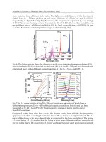
When the transverse laser intensity is increased above a certain value at unequal detunings,
we now observe the appearance of novel SDTs. In Fig. 17, the fluorescence images of the
trapped atoms, obtained with I
t
≡ I
x
+ I
y
= 11.4I
z
fixed, are presented for various values of
δ
t
–
δ
z
. The central peak, corresponding to the usual SDT, becomes weak when the detunings
are different, as discussed in Fig. 16(b). However, the two side peaks, associated with the
novel SDTs, are displaced symmetrically with respect to the MOT center, in proportion to
δ
t
–
δ

z
. In addition to these two adjustable side SDTs, there also exist another two weak SDTs
located midway between each side SDT and the central one, which will be discussed later.


Fig. 17. (a) Fluorescence images that show two adjustable side SDTs for several values of
δ
t
–
δ
z
. (b) SDT pictures plotted in series with the increasing detuning differences.
In Fig. 18(a), we plot the positions of the two side SDTs for various values of
δ
t
–
δ
z
,
represented by filled squares, which are also shown in Fig. 17(b). Attributed to the
coherences between the ground-state magnetic sublevels with
Δm = ±1 transitions (see Fig.
18(b)), the two side SDTs appear at the positions
(
)
(
)
=/
StzgB
zgb

δδ μ
±− and thus their
separation satisfies,
=,
S
B
g
zh
bg
νμ
Δ
±
Δ
(18)
where
Δ
ν
= (
δ
t
–
δ
z
)/(2
π
) and
μ
B
is the Bohr magneton. Since the ground-state g-factor is g
g

=
1/3 for
85
Rb atoms and the magnetic field gradient is b = 0.17 T/m, the calculated value
An Asymmetric Magneto-Optical Trap

407
(solid line) is Δz/Δ
ν
= 1.26 mm/MHz, which agrees well with the experimental result of 1.25
(
±0.12) mm/MHz, considering 10% error of position measurements. On the other hand, the
two weak SDTs, resulting from the coherences due to
Δm = ±2 transitions (refer to Fig.
18(b)), are located midway at z
M
= z
S
/2, as shown in Fig. 18(a) (open circles). The fitted result
is 0.61 mm/MHz, which is almost half the value given by Eq. (18), in good agreement with
the ‘doubled’ energy differences of the
Δm = ±2 transitions with respect to the Δm = ±1 ones,
responsible for the side SDTs.


(a) (b)
Fig. 18. Measured positions of available SDTs versus negative detuning differences.
In order to have a qualitative understanding of the detuning-difference dependence, we
have calculated the cooling and trapping forces in two dimension by using the optical Bloch
equation approach (Dalibard, 1988; Chang & Minogin, 2002; Noh & Jhe, 2007). In Fig. 19(a),

we present the calculated forces F(z,v = 0) for F
g
= 3→ F
e
= 4 atomic transition. In the
presence of the transverse lasers, the ground-state sublevels with Δm = ±1 transitions can be
coupled by a
π
photon from the transverse lasers in combination with a
σ
±
photon from the
longitudinal lasers (see Fig. 18(b)). As a result, for unequal detunings, there exists a position
where the Zeeman shift compensates the laser-frequency difference, such that


(a) (b)
Fig. 19. (a) Calculated forces F(z,v =0) for various detuning differences. The maximum forces
at 0.3
Γ corresponds to 5 × 10
–3
 kΓ. Here
δ
z
= –2.7Γ, I
z
= 0.11 mW/cm
2
, and I
t

= 5.6I
z
. (b)
Five SDTs, including two weak SDTs midway between the two side SDTs and the central
one, for
δ
t
–
δ
z
= –0.24Γ.
Recent Optical and Photonic Technologies

408

=.
zt gB
g
bz
ω
ωμ
−
± (19)
At this position, atoms can feel the sub-Doppler forces associated with the
Δm = ±1
coherences and thus the novel SDT is obtained at two positions of
±

(
δ

x
–
δ
z
)/(g
g
μ
B
b), as
confirmed in Fig. 18(a). As shown in Fig. 19(b), the two weak midway SDTs arise because
the weak
σ
±
photons, in addition to the dominant
π
ones, from the transverse lasers can
contribute to the atomic coherences in the z-direction. Therefore, besides the
Δm = ±1
transitions responsible for the side SDTs, the two-photon-assisted
Δm = ±2 coherences (here,
each
σ
±
photon comes from the longitudinal and the transverse laser, as shown in Fig. 18(b))
can be generated, and atoms at the position z
M
, satisfying the relation

ω
t

–

ω
z
=
±2g
g
μ
B
bz
M
, feel this additional coherence. As a result, the midway SDTs can be obtained at
z
M
= z
S
/2 (see Fig. 18(a)). The typically observed image and the calculated force are
presented in Fig. 19(b).
5. Conclusions
In this article we have presented experimental and theoretical works on the asymmetric
magneto-optical trap. In Sec. 2, we have studied parametric resonance in a magneto-optical
trap. We have described a theoretical aspect of parametric resonance by the analytic and
numerical methods. We also have measured the amplitude and phase of the limit cycle
motions by changing the modulation frequency or the amplitude. We find that the results
are in good agreement with the calculation results, which are based on simple Doppler
cooling theory. In the final subsection we described direct observation of the sub-Doppler
part of the MOT without the Doppler part by using the parametric resonance which. We
compared the spatial profile of sub-Doppler trap with the Monte-Carlo simulation, and
observed they are in good agreements.
In Sec. 3, we have presented two methods to measure the trap frequency: one is using

parametric resonance and the other transient oscillation method. In the case of parametric
resonance method, we could measure the trap frequency accurately by decreasing the
modulation amplitude of the parametric excitation down to its threshold value. While only
the trap frequency were able to be obtained by the parametric resonance method, we could
obtain both the trap frequency and the damping coefficient by the transient oscillation
method. We have made a quantitative study of the Doppler cooling theory in the MOT by
measuring the trap parameters. We have found that the simple rate-equation model can
accurately describe the experimental data of trap frequencies.
In Sec. 4, we have demonstrated the adjustable multiple traps in the MOT. When the laser
detunings are different, the usual sub-Doppler force and the corresponding damping
coefficient at the MOT center is greatly suppressed, whereas the novel sub-Doppler traps are
generated and exist within a finite range of detuning differences. We have found that
π
and
σ
±
atomic transitions excited by the transverse lasers in the longitudinal direction are
responsible for the strong side and the weak middle sub-Doppler traps, respectively. The
adjustable array of sub-Doppler traps may be useful for controllable atom-interferometer-
type experiments in atom optics or quantum optics.
The AMOT described in this article can be used for study of nonlinear dynamics using cold
atoms such as critical phenomena far from equilibrium (Kim et al., 2006) or a nonlinear
Duffing oscillation (Nayfeh & Moore, 1979; Strogatz, 2001).
An Asymmetric Magneto-Optical Trap

409
6. Acknowledgement
This work was supported by the Korea Research Foundation Grant funded by the Korean
Government (KRF-2008-313-C00355).
7. References

Bagnato, V. S., Marcassa, L. G., Oria, M., Surdutovich, G. I., Vitlina, R. & Zilio, S. C. (1993). Spatial
distribution of atoms in a magneto-optical trap, Phys. Rev. A Vol. 48(No. 5): 3771–3775.
Chang, S. & Minogin, V. (2002). Density-matrix approach to dynamics of multilevel atoms in
laser fields, Phys. Rep. Vol. 365(No. 2): 65–143.
Dalibard, J. (1998). Laser cooling of an optically thick gas: The simplest radiation pressure
trap?, Opt. Commun. Vol. 68(No. 3): 203–208.
di Stefano, A., Fauquembergue, M., Verkerk, P. & Hennequin, D. (2003). Giant oscillations in
a magneto-optical trap, Phys. Rev. A Vol. 67(No. 3): 033404-1–033404-4.
Dias Nunes, F., Silva, J. F., Zilio, S. C. & Bagnato, V. S. (1996). Influence of laser fluctuations
and spontaneous emission on the ring-shaped atomic distribution in a magneto-
optical trap, Phys. Rev. A Vol. 54(No. 3): 2271–2274.
Drewsen, M., Laurent, Ph., Nadir, A., Santarelli, G., Clairon, A., Castin, Y., Grinson, D. &
Salomon, C. (1994). Investigation of sub-Doppler cooling effects in a cesium
magnetooptical trap, Appl. Phys. B Vol. 59(No. 3): 283–298.
Friebel, S., D’Andrea, C., Walz, J., Weitz, M. & H¨ansch, T. W. (1998). CO
2
-laser optical
lattice with cold rubidium atoms, Phys. Rev. A Vol. 57(No. 1): R20–R23.
Heo, M. S., Kim, K., Lee, K. H., Yum, D., Shin, S., Kim, Y., Noh, H. R. & Jhe, W. (2007).
Adjustable multiple sub-Doppler traps in an asymmetric magneto-optical trap,
Phys. Rev. A Vol. 75(No. 2): 023409-1–023409-4.
Hope, A., Haubrich, D., Muller, G., Kaenders, W. G. & Meschede, D. (1993). Neutral cesium
atoms in strong magnetic-quadrupole fields at sub-doppler temperatures, Europhys.
Lett. Vol. 22(No. 9): 669–674.
Jun, J. W., Chang, S., Kwon, T. Y., Lee, H. S. & Minogin, V. G. (1999). Kinetic theory of the
magneto-optical trap for multilevel atoms, Phys. Rev. A Vol. 60(No. 5): 3960–3972.
Kim, K., Noh, H. R., Yeon, Y. H. & Jhe,W. (2003). Observation of the Hopf bifurcation in
parametrically driven trapped atoms, Phys. Rev. A Vol. 68(No. 3): 031403(R)-1–
031403(R)-4.
Kim, K., Noh, H. R. & Jhe, W. (2004). Parametric resonance in an intensity-modulated

magneto-optical trap, Opt. Commun. Vol. 236(No. 4-6): 349–361.
Kim, K., Noh, H. R., Ha, H. J. & Jhe, W. (2004). Direct observation of the sub-Doppler trap in
a parametrically driven magneto-optical trap, Phys. Rev. A Vol. 69(No. 3): 033406-1–
033406-5.
Kim, K., Noh, H. R. & Jhe, W. (2005). Measurements of trap parameters of a magneto-optical
trap by parametric resonance, Phys. Rev. A Vol. 71(No. 3): 033413-1–033413-5.
Kim, K., Lee, K. H., Heo, M., Noh, H. R. & Jhe, W. (2005). Measurement of the trap
properties of a magneto-optical trap by a transient oscillation method, Phys. Rev. A
Vol. 71(No. 5): 053406-1–053406-5.
Kim, K., Heo, M. S., Lee, K. H., Jang, K., Noh, H. R., Kim, D. & Jhe, W. (2006). Spontaneous
Symmetry Breaking of Population in a Nonadiabatically Driven Atomic Trap: An
Ising-Class Phase Transition, Phys. Rev. Lett. Vol. 96(No. 15): 150601-1–150601-4.
Kohns, P., Buch, P., Suptitz, W., Csambal, C. & Ertmer, W. (1993). On-Line Measurement of
Sub-Doppler Temperatures in a Rb Magneto-optical Trap-by-Trap Centre
Oscillations, Europhys. Lett. Vol. 22(No. 7): 517–522.
Recent Optical and Photonic Technologies

410
Kulin, S., Killian, T. C., Bergeson, S. D. & Rolston, S. L. (2000). Plasma Oscillations and
Expansion of an Ultracold Neutral Plasma, Phys. Rev. Lett. Vol. 85(No. 2): 318–321.
Labeyrie, G., Michaud, F. & Kaiser, R. (2006). Self-Sustained Oscillations in a Large
Magneto-Optical Trap, Phys. Rev. Lett. Vol. 96(No. 2): 023003-1–023003-4.
Landau, L. D. & Lifshitz, E. M. (1976). Mechanics, Pergamon, London.
Lapidus, L. J., Enzer, D. & Gabrielse, G. (1999). Stochastic Phase Switching of a
Parametrically Driven Electron in a Penning Trap, Phys. Rev. Lett. Vol. 83(No. 5):
899–902.
Metcalf, H. J. & van der Straten, P. (1999). Laser Cooling and Trapping, Springer, New York.
Nayfeh, N. H. & Moore, D. T. (1979). Nonlinear Oscillations, Wiley, New York.
Noh, H. R. & Jhe, W. (2007). Semiclassical theory of sub-Doppler forces in an asymmetric
magneto-optical trap with unequal laser detunings, Phys. Rev. A Vol. 75(No. 5):

053411-1–053411-9.
Raab, E. L., Prentiss, M., Cable, A., Chu, S. & Pritchard, D. E. (1987). Trapping of Neutral
Sodium Atoms with Radiation Pressure, Phys. Rev. Lett. Vol. 59(No. 23): 2631–2634.
Razvi, M. A. N., Chu, X. Z., Alheit, R., Werth, G. & Blümel, R. (1998). Fractional frequency
collective parametric resonances of an ion cloud in a Paul trap, Phys. Rev. A Vol.
58(No. 1): R34–R37.
Sesko, D., Walker, T. & Wieman, C. (1991). Behavior of neutral atoms in a spontaneous force
trap, J. Opt. Soc. Am. B Vol. 8(No. 5): 946–958.
Steane, A. M., Chowdhury, M. & Foot, C. J. (1992). Radiation force in the magneto-optical
trap, J. Opt. Soc. Am. B Vol. 9(No. 12): 2142–2158.
Strogatz, S. H. (2001). Nonlinear Dynamics and Chaos, Perseus, New York.
Tabosa, J. W. R., Chen, G., Hu, Z., Lee, R. B. & Kimble, H. J. (1991). Nonlinear spectroscopy
of cold atoms in a spontaneous-force optical trap, Phys. Rev. Lett. Vol. 66(No. 25):
3245–3248.
Tan, J. & Gabrielse, G. (1991). Synchronization of parametrically pumped electron oscillators
with phase bistability, Phys. Rev. Lett. Vol. 67(No. 22): 3090–3093.
Tan, J. & Gabrielse, G. (1993). Parametrically pumped electron oscillators, Phys. Rev. A Vol.
48(No. 4): 3105–3121.
Townsend, C. G., Edwards, N. H., Cooper, C. J., Zetie, K. P., Foot, C. J., Steane, A. M.,
Szriftgiser, P., Perrin, H. & Dalibard. J. (1995). Phase-space density in the magneto-
optical trap, Phys. Rev. A Vol. 52(No. 2): 1423–1440.
Walhout, M., Dalibard, J., Rolston, S. L. & Phillips, W. D. (1992).
σ
+
–
σ
–
Optical molasses in a
longitudinal magnetic field, J. Opt. Soc. Am. B Vol. 9(No. 11): 1997–2007.
Tseng, C. H., Enzer, D., Gabrielse, G. & Walls, F. L. (1999). 1-bit memory using one electron:

Parametric oscillations in a Penning trap, Phys. Rev. A Vol. 59(No. 3): 2094–2104.
Walker, T., Sesko, D. & Wieman, C. (1990). Collective behavior of optically trapped neutral
atomstitle, Phys. Rev. Lett. Vol. 64(No. 4): 408–411.
Walker, T. & Feng, P. (1994). Measurements of Collisions Between Laser-Cooled Atoms,
Adv. At. Mol. Opt. Phys. Vol. 34: 125–170.
Wallace, C. D., Dinneen, T. P., Tan, K. Y. N., Kumarakrishnan, A., Gould, P. L. & Javanainen,
J. (1994). Measurements of temperature and spring constant in a magneto-optical
trap, J. Opt. Soc. Am. B Vol. 11(No. 5): 703–711.
Wilkowski, D., Ringot, J., Hennequin, D. & Garreau, J. C. (2000). Instabilities in a
Magnetooptical Trap: Noise-Induced Dynamics in an Atomic System, Phys. Rev.
Lett. Vol. 85(No. 9): 1839–1842.
Xu, X., Loftus, T. H., Smith, M. J., Hall, J. L., Gallagher, A. & Ye, J. (2002). Dynamics in a two-
level atom magneto-optical trap, Phys. Rev. A Vol. 66(No. 1): 011401-1–011401-4.
20
The Photonic Torque Microscope:
Measuring Non-conservative Force-fields
Giovanni Volpe
1,2,3
, Giorgio Volpe
1
and Giuseppe Pesce
4

1
ICFO – The Institute of Photonic Sciences, Castelldefels (Barcelona),
2
Max-Planck-Institut für Metallforschung, Stuttgart,
3
Universität Stuttgart, Stuttgart,
4

Università di Napoli “Federico II”, Napoli,
1
Spain
2,3
Germany
4
Italy
1. Introduction
Over the last 20 years the advances of laser technology have permitted the development of
an entire new field in optics: the field of optical trapping and manipulation. The focal spot of a
highly focused laser beam can be used to confine and manipulate microscopic particles
ranging from few tens of nanometres to few microns (Ashkin, 2000; Neuman & Block, 2004).


Fig. 1. PFM setups with detection using forward (a) and backward (b) scattered light.
Such an optical trap can detect and measure forces and torques in microscopic systems – a
technique now known as photonic force microscope (PFM). This is a fundamental task in
many areas, such as biophysics, colloidal physics and hydrodynamics of small systems.
Recent Optical and Photonic Technologies

412
The PFM was devised in 1993 (Ghislain & Webb, 1993). A typical PFM comprises an optical
trap that holds a probe – a dielectric or metallic particle of micrometre size, which randomly
moves due to Brownian motion in the potential well formed by the optical trap – and a
position sensing system. The analysis of the thermal motion provides information about the
local forces acting on the particle (Berg-Sørensen & Flyvbjerg, 2004). The PFM can measure
forces in the range of femtonewtons to piconewtons. This range is well below the limits of
techniques based on micro-fabricated mechanical cantilevers, such as the atomic force
microscope (AFM).
However, an intrinsic limit of the PFM is that it can only deal with conservative force-fields,

while it cannot measure the presence of a torque, which is typically associated with the
presence of a non-conservative (or rotational) force-field.
In this Chapter, after taking a glance at the history of optical manipulation, we will briefly
review the PFM and its applications. Then, we will discuss how the PFM can be enhanced to
deal with non-conservative force-fields, leading to the photonic torque microscope (PTM)
(Volpe & Petrov, 2006; Volpe et al., 2007a). We will also present a concrete analysis
workflow to reconstruct the force-field from the experimental time-series of the probe
position. Finally, we will present three experiments in which the PTM technique has been
successfully applied:
1.

Characterization of singular points in microfluidic flows. We applied the PTM to
microrheology to characterize fluid fluxes around singular points of the fluid flow
(Volpe et al., 2008).
2. Detection of the torque carried by an optical beam with orbital angular momentum. We used the
PTM to measure the torque transferred to an optically trapped particle by a Laguerre-
Gaussian beam (Volpe & Petrov, 2006).
3. Quantitative measurement of non-conservative forces generated by an optical trap. We used the
PTM to quantify the contribution of non-conservative optical forces to the optical
trapping (Pesce et al., 2009).
2. Brief history of optical manipulation
Optical trapping and manipulation did not exist before the invention of the laser in 1960
(Townes, 1999). It was already known from astronomy and from early experiments in optics
that light had linear and angular momentum and, therefore, that it could exert radiation
pressure and torques on physical objects. Indeed, light’s ability to exert forces has been
recognized at least since 1619, when Kepler’s De Cometis described the deflection of comet
tails by sunrays.
In the late XIX century Maxwell’s theory of electromagnetism predicted that the light
momentum flux was proportional to its intensity and could be transferred to illuminated
objects, resulting in a radiation pressure pushing objects along the propagation direction of

light.
Early exciting experiments were performed in order to verify Maxwell’s predictions. Nichols
and Hull (Nichols & Hull, 1901) and Lebedev (Lebedev, 1901) succeeded in detecting
radiation pressure on macroscopic objects and absorbing gases. A few decades later, in 1936,
Beth reported the experimental observation of the torque on a macroscopic object resulting
from interaction with light (Beth, 1936): he observed the deflection of a quartz wave plate
suspended from a thin quartz fibre when circularly polarized light passed through it. These
effects were so small, however, that they were not easily detected. Quoting J. H. Poynting’s
The Photonic Torque Microscope: Measuring Non-conservative Force-fields

413
presidential address to the British Physical Society in 1905, “a very short experience in
attempting to measure these forces is sufficient to make one realize their extreme
minuteness – a minuteness which appears to put them beyond consideration in terrestrial
affairs.” (Cited in Ref. (Ashkin, 2000))
Things changed with the invention of the laser in the 1960s (Townes, 1999). In 1970 Ashkin
showed that it was possible to use the forces of radiation pressure to significantly affect the
dynamics of transparent micrometre sized particles (Ashkin, 1970). He identified two basic
light pressure forces: a scattering force in the direction of the incident beam and a gradient
force in the direction of the intensity gradient of the beam. He showed experimentally that,
using just these forces, a focused laser beam could accelerate, decelerate and even stably
trap small micrometre sized particles.
Ashkin considered a beam of power
P reflecting on a plane mirror: /Ph
ν
photons per
second strike the mirror, each carrying a momentum
/hc
ν
, where

h
is the Planck constant,
ν
is the light frequency and
c
the speed of light. If they are all reflected straight back, the
total change in light momentum per second is
(
)
(
)
2/ / 2/Ph h c Pc
νν
⋅⋅=, which, by
conservation of momentum, implies that the mirror experiences an equal and opposite force
in the direction of the light. This is the maximum force that one can extract from the light.
Quoting Ashkin (Ashkin, 2000), “Suppose we have a laser and we focus our one watt to a
small spot size of about a wavelength 1 m
μ
≅
, and let it hit a particle of diameter also of
1 m
μ
. Treating the particle as a 100% reflecting mirror of density
3
1/
g
mcm≅ , we get an
acceleration of the small particle

31292
/ 10 /10 10 /AFm d
y
nes
g
mcmsec
−−
== = = . Thus,
6
10A
g
≅ , where
32
10 /
g
cm sec≅ , the acceleration of gravity. This is quite large and should
give readily observable effects, so I tried a simple experiment. [ ] It is surprising that this
simple first experiment [ ], intended only to show forward motion due to laser radiation
pressure, ended up demonstrating not only this force but the existence of the transverse
force component, particle guiding, particle separation, and stable 3D particle trapping.”
In 1986, Ashkin and colleagues reported the first observation of what is now commonly
referred to as an optical trap (Ashkin et al., 1986): a tightly focused beam of light capable of
holding microscopic particles in three dimensions. One of Ashkin’s co-authors, Steven Chu,
would go on to use optical tweezing in his work on cooling and trapping atoms. This
research earned Chu, together with Claude Cohen-Tannoudji and William Daniel Phillips,
the 1997 Nobel Prize in Physics.
In the late 1980s, the new technology was applied to the biological sciences, starting by
trapping tobacco mosaic viruses and Escherichia coli bacteria. In the early 1990s, Block,
Bustamante and Spudich pioneered the use of optical trap force spectroscopy, an alternate
name for PFM, to characterize the mechanical properties of biomolecules and biological

motors (Block et al., 1990; Finer et al., 1994; Bustamante et al., 1994). Optical traps allowed
these biophysicists to observe the forces and dynamics of nanoscale motors at the single-
molecule level. Optical trap force spectroscopy has led to a deeper understanding of the
nature of these force-generating molecules, which are ubiquitous in nature.
Optical tweezers have also proven useful in many other areas of physics, such as atom
trapping (Metcalf & van der Straten, 1999) and statistical physics (Babic et al., 2005).
3. The photonic force microscope
One of the most prominent uses of optical tweezers is to measure tiny forces, in the order of
100s of femtonewtons to 10s of piconewtons. A typical PFM setup comprises an optical trap
Recent Optical and Photonic Technologies

414
to hold a probe - a dielectric or metallic particle of micrometer size - and a position sensing
system. In the case of biophysical applications the probe is usually a small dielectric bead
tethered to the cell or molecule under study. The probe randomly moves due to Brownian
motion in the potential well formed by the optical trap. Near the centre of the trap, the
restoring force is linear in the displacement. The stiffness of such harmonic potential can be
calibrated using the three-dimensional position fluctuations. To measure an external force
acting on the probe it suffices to measure the probe average position displacement under the
action of such force and multiply it by the stiffness.
In order to understand the PFM it is necessary to discuss these three aspects:
1.
the optical forces that act on the probe and produce the optical trap;
2.
the position detection, which permits one to track the probe position with nanometre
resolution and at kilohertz sampling rate;
3.
the statistics of the Brownian motion of the probe in the trap, which are used in the
calibration procedure.
3.1 Optical forces

It is well known from quantum mechanics that light carries a momentum: for a photon at
wavelength
λ
the associated momentum is /ph
λ
=
. For this reason, whenever an atom
emits or absorbs a photon, its momentum changes according to Newton’s laws. Similarly, an
object will experience a force whenever a propagating light beam is refracted or reflected by
its surface. However, in most situations this force is much smaller than other forces acting
on macroscopic objects so that there is no noticeable effect and, therefore, can be neglected.
The objects, for which this radiation pressure exerted by light starts to be significant, weigh
less than
1 g
μ
and their size is below 10s of microns.
A focused laser beam acts as an attractive potential well for a particle. The equilibrium
position lies near – but not exactly at – the focus. When the object is displaced from this
equilibrium position, it experiences an attractive force towards it. In first approximation this
restoring force is proportional to the displacement; in other words, optical tweezers force
can generally be described by Hooke’s law:

(
)
0
,
xx
Fkxx=− − (1)
where x is the particle’s position, x
0

is the focus position and k
x
is the spring constant of the
optical trap along the x -direction, usually referred to as trap stiffness. In fact, an optical
tweezers creates a three-dimensional potential well, which can be approximated by three
independent harmonic oscillators, one for each of the x -, y- and z-directions. If the optics are
well aligned, the x and y spring constants are roughly the same, while the z spring constant
is typically smaller by a factor of 5 to 10.
Considering the ratio between the characteristic dimension L of the trapped object and the
wavelength
λ
of the trapping light, three different trapping regimes can be defined:
1. the Rayleigh regime, when L
λ
<
< ;
2. an intermediate regime, when L is comparable to
λ
;
3. the geometrical optics regime, when L
λ
>> .
In Fig. 2 an overview of the kind of objects belonging to each of these regimes is presented,
considering that the trapping wavelength is usually in the visible or near-infrared spectral
region. In any of these regimes, the electromagnetic equations can be solved to evaluate the
The Photonic Torque Microscope: Measuring Non-conservative Force-fields

415
force acting on the object. However, this can be a cumbersome task. For the Rayleigh regime
and geometrical optics regime approximate models have been developed. However, most of

the objects that are normally trapped in optical manipulation experiments fall in the
intermediate regime, where such approximations cannot be used. In particular, this is true
for the probes usually used for the PFM: typically particles with diameter between 0.1 and
10 micrometres.


Fig. 2. Trapping regimes and objects that are typically optically manipulated: from cells to
viruses in biophysical experiments, and from atoms to colloidal particles in experimental
statistical physics. The wavelength of the trapping light is usually in the visible or near-
infrared.
3.2 Position detection
The three-dimensional position of the probe is typically measured through the scattering of
a light beam illuminating it. This can be the same beam used for trapping or an auxiliary
beam.
Typically, position detection is achieved through the analysis of the interference of the
forward-scattered (FS) light and unscattered (incident) light. A typical setup is shown in Fig.
Recent Optical and Photonic Technologies

416
1(a). The PFM with FS detection was extensively studied, for example, in Ref (Rohrbach &
Stelzer, 2002).
In a number of experiments, however, geometrical constraints may prevent access to the FS
light, forcing one to make use of the backward-scattered (BS) light instead. This occurs, for
example, in biophysical applications where one of the two faces of a sample holder needs to
be coated with some specific material or in plasmonics applications where a plasmon wave
needs to be coupled to one of the faces of the holder (Volpe et al., 2006). A typical setup that
uses the BS light is presented in Fig. 1(b). The PFM with BS detection has been studied
theoretically in Ref. (Volpe et al., 2007b) and experimentally in Ref. (Huisstede et al., 2005).
Two types of photodetectors are typically used. The quadrant photodetector (QPD) works
by measuring the intensity difference between the left-right and top-bottom sides of the

detection plane. The position sensing detector (PSD) measures the position of the centroid of
the collected intensity distribution, giving a more adequate response for non-Gaussian
profiles. Note that high-speed video systems are also in use, but they do not achieve the
acquisition rate available with photodetectors.
3.3 Brownian motion of an optically trapped particle
Assuming a very low Reynolds number regime (Happel & Brenner, 1983), the Brownian
motion of the probe in the optical trap is described by a set of Langevin equations:

() () 2 (),ttDt
γγ
′+ =rKr h (2)
where
[]
() (), (), ()
T
txt
y
tzt=r is the probe position,
6 R
γ
πη
=
its friction coefficient, R its
radius,
η
the medium viscosity, K the stiffness matrix, 2(),(),()
T
xyz
D hththt
γ

⎡
⎤
⎣
⎦
a vector of
independent white Gaussian random processes describing the Brownian forces, /
B
DkT
γ
=
the diffusion coefficient, T the absolute temperature and
B
k the Boltzmann constant. The
orientation of the coordinate system can be chosen in such a way that the restoring forces
are independent in the three directions, i.e.
(
)
diag , ,
x
y
z
kkk=K
. In such reference frame the
stochastic differential Eqs. (2) are separated and, without loss of generality, the treatment
can be restricted to the x-projection of the system.
When a constant and homogeneous external force
,ext x
f
acting on the probe produces a shift
in its equilibrium position in the trap, its value can be obtained as:

,
(),
ext x x
f
kxt=
(3)
where
()xt is the probe mean displacement from the equilibrium position.
There are several straightforward methods to experimentally measure the trap parameters –
trap stiffness and conversion factor between voltage and length – and, therefore, the force
exerted by the optical tweezers on an object, without the need for a theoretical reference
model of the electromagnetic interaction between the particle and the laser beam. The most
commonly employed ones are the drag force method, the equipartition method, the potential
analysis method and the power spectrum or correlation method (Visscher et al., 1996; Berg-
Sørensen & Flyvbjerg, 2004). The latter, in particular, is usually considered the most reliable
one. Experimentally the trap stiffness can be found by fitting the autocorrelation function
(ACF) of the Brownian motion in the trap obtained from the measurements to the theoretical
one, which reads
The Photonic Torque Microscope: Measuring Non-conservative Force-fields

417

*
() ( ) () .
x
k
B
xx
x

kT
rxtxt e
k
τ
γ
ττ
−
=+ = (4)
4. The photonic torque microscope
The PFM measures a constant force acting on the probe. This implies that the force-field to
be measured has to be invariable (homogeneous) on the scale of the Brownian motion of the
trapped probe, i.e. in a range of 10s to 100s of nanometres depending on the trapping
stiffness. In particular, as we will see, this condition implicates that the force-field must be
conservative, excluding the possibility of a rotational component.


Fig. 3. Examples of physical systems that produce force-fields that cannot be correctly
probed with a classical PFM, because they vary on the scale of the Brownian motion of the
trapped probe (a possible range is indicated by the red bars): (a) forces produced by a
surface plasmon polariton in the presence of a patterned surface on a 50nm radius dielectric
particle (adapted from Ref. (Quidant et al., 2005)); (b) trapping potential for 10nm diameter
dielectric particle near a 10nm wide gold tip in water illuminated by a 810nm
monochromatic light beam (adapted from Ref. (Novotny et al., 1997)); and (c) force-field
acting on a 500nm radius dielectric particle in the focal plane of a highly focused Laguerre-
Gaussian beam (adapted from Ref. (Volpe & Petrov, 2006)).
However, there are cases where these assumptions are not fulfilled. The force-field can vary
in the nanometre scale, for example, considering the radiation forces exerted on a dielectric
particle by a patterned optical near-field landscape at an interface decorated with resonant
gold nanostructures (Quidant et al., 2005) (Fig. 3 (a)), the nanoscale trapping that can be
achieved near a laser-illuminated tip (Novotny et al., 1997) (Fig. 3(b)), the optical forces

produced by a beam which carries orbital angular momentum (Volpe & Petrov, 2006) (Fig.
3(c)), or in the presence of fluid flows (Volpe et al., 2008). In order to deal with these cases,
we need a deeper understanding of the Brownian motion of the optically trapped probe in
the trapping potential.
In the following we will discuss the Brownian motion near an equilibrium point in a force-
field and we will see how this permits us to develop a more powerful theory of the PFM: the
Photonic Torque Microscope (PTM). Full details can be found in Ref. (Volpe et al., 2007a).
Recent Optical and Photonic Technologies

418
4.1 Brownian motion near an equilibrium position
In the presence of an external force-field
(
)
()
ext
tfr , Eq. (2) can be written in the form:

(
)
() () 2 (),ttDt
γγ
′+ =rfr h (5)
where the total force acting on the probe
(
)
(
)
() () ()
ext

ttt=−fr f r Kr depends on the position of
the probe itself, but does not vary over time.
The force
() ()()
() (), ()
T
xy
tftft
⎡
⎤
=
⎣
⎦
fr r r
can be expanded in Taylor series up to the first order
around an arbitrary point
r
0
:

()
()
()
(
)
(
)
() ()
()
()

() () () ,
xx
x
y
yy
ff
xy
f
ttot
f
ff
xy
∂∂
∂∂
∂∂
∂∂
⎡⎤
⎢⎥
⎡⎤
⎢⎥
=+ −+−
⎢⎥
⎢⎥
⎢⎥
⎣⎦
⎢⎥
⎢⎥
⎣⎦
00
0

00
0
00
rr
r
fr r r r r
r
rr
(6)
where
0
r
f and
0
r
J
are the zeroth-order and first-order expansion coefficients, i.e. the force-
field value at the point
0
r and the Jacobian of the force-field calculated in
0
r . In the
following we will assume, without loss of generality,
0
=
0
r .
In a PFM the probe is optically trapped and, therefore, it diffuses due to Brownian motion in
the total force-field (the sum of the optical trapping force and external force-fields). If
0≠

0
r
f , the probe experiences a shift in the direction of the force and, after a transient time
has elapsed, the particle settles down in a new equilibrium position of the total force-field,
such that 0=
0
r
f . As we have already seen, the measurement of this shift allows one to
evaluate the homogeneous force acting on the probe in the standard PFM and, therefore, the
zeroth order term of the Taylor expansion. In the following we will assume this to be null
and study the statistics of the Brownian motion near the equilibrium point can be analyzed
in order to reconstruct the force-field up to its first-order approximation.
4.2 Conservative and rotational components of the force-field
The first order approximation to Eq. (5) near an equilibrium point of the force-field, 0=r

, is:

1
() () 2 (),ttDt
γ
−
′= +
0
rJr h (7)
where
[]
() (), ()
T
txt
y

t=r , () (), ()
T
xy
ththt
⎡
⎤
=
⎣
⎦
h and
0
J
is the Jacobian calculated at the
equilibrium point.
According to the Helmholtz theorem, any force-field can be separated into its conservative
(irrotational) and non-conservative (rotational or solenoidal) components. With simple
algebraic passages, the Jacobian
J
0
can be written as the sum of two matrices:

,
=
+
0cnc
J
JJ (8)
where

()

() ()
1
2
() ()
()
1
2
y
xx
yy
x
f
ff
xyx
ff
f
xy y
∂
∂∂
∂∂∂
∂∂
∂
∂∂ ∂
⎡
⎤
⎛⎞
+
⎢
⎥
⎜⎟

⎢
⎥
⎝⎠
=
⎢
⎥
⎛⎞
⎢
⎥
+
⎜⎟
⎢
⎥
⎝⎠
⎣
⎦
c
0
00
J
00
0
(9)
The Photonic Torque Microscope: Measuring Non-conservative Force-fields

419
and

()
()

1
0
2
.
()
()
1
0
2
y
x
y
x
f
f
yx
f
f
xy
∂
∂
∂∂
∂
∂
∂∂
⎡
⎤
⎛⎞
−
⎢

⎥
⎜⎟
⎢
⎥
⎝⎠
=
⎢
⎥
⎛⎞
⎢
⎥
−
⎜⎟
⎢
⎥
⎝⎠
⎣
⎦
nc
0
0
J
0
0
(10)
It is easy to show that
J
c
is the conservative component of the force-field and that J
nc

is the
rotational component.
The two components can be easily identified if the coordinate system is chosen such that
()
()
y
x
f
f
y
x
∂
∂
∂∂
=−
0
0
. In this case, the Jacobian J
0
normalized by the friction coefficient
γ
reads:

1
,
x
y
φ
γ
φ

−
−Ω
⎡
⎤
=
⎢
⎥
−Ω −
⎣
⎦
0
J (11)
where
/
xx
k
φ
γ
= , /
yy
k
φ
γ
=
,
()
x
x
f
k

x
∂
∂
=−
0
,
()
y
y
f
k
y
∂
∂
=−
0
and
Ω
=
1
()
x
f
y
∂
γ
∂
−
=
0

1
()
y
f
x
∂
γ
∂
−
−
0
.
In Eq. (11) the rotational component, which is invariant under a coordinate rotation, is
represented by the non-diagonal terms of the matrix:
Ω
is the value of the constant angular
velocity of the probe rotation around the z-axis due to the presence of the rotational force-
field. The conservative component, instead, is represented by the diagonal terms of the
Jacobian and is centrally symmetric with respect to the origin. Without loss of generality, it
can be imposed that the stiffness of the trapping potential is higher along the x-axis, i.e.
x
y
kk> and, therefore,
x
y
φ
φ
> .
4.3 Stability study
The conditions for the stability of the equilibrium point are

()
()
222
Det 0
,
Tr 2 0
φφ
φ
⎧
=
−Δ +Ω >
⎪
⎨
=− <
⎪
⎩
0
0
J
J
(12)
where
()
2
xy
φφφ
=+ and
(
)

2
xy
φφφ
Δ= − . The fundamental condition required to achieve
the stability is 0
φ
> . Assuming that this condition is satisfied, the behaviour of the optically
trapped probe can be explored as a function of the parameters /
φ
Ω
and /
φ
φ
Δ . The
stability diagram is shown in Fig. 4(a).
The standard PFM corresponds to
0
φ
Δ
=
and 0
Ω
= . When a rotational term is added, i.e.
0
Ω≠ and 0
φ
Δ= , the system remains stable. When there is no rotational contribution to
the force-field ( 0
Ω
= ) the equilibrium point becomes unstable as soon as

φ
φ
Δ≥ . This
implicates that 0
y
φ
<
and, therefore, the probe is not confined in the

y
-direction any more.
In the presence of a rotational component ( 0
Ω
≠ ) the stability region becomes larger; the
equilibrium point now becomes unstable only for
22
φφ
Δ
≥−Ω.
Recent Optical and Photonic Technologies

420



Fig. 4. (a) Stability diagram. Assuming φ > 0, the stability of the system is shown as a
function of the parameters /
φ
Ω
and /

φ
φ
Δ
. The white region satisfies the stability
conditions in Eq. (12). The dashed lines represent the
||
φ
Δ
=Ω and
φ
φ
Δ
= curves. The dots
represent the parameters that are further investigated in Figs. 4(b) and 5. (b) Brownian
motion near an equilibrium point. The arrows show the force-field vectors for various
values of the parameters /
φ
Ω
and /
φ
φ
Δ
. The shadowed areas show the probability
distribution function (PDF) of the probe position in the corresponding force-field.

Some examples of possible force-fields are presented in Fig. 4(b). When 0
Ω
= the probe
movement can be separated along two orthogonal directions. As the value of
φ

Δ increases,
the probability density function (PDF) of the probe position becomes more and more
elliptical, until for
φ
φ
Δ
≥ the probe is confined only along the x-direction and the
confinement along the
y-direction is lost.
If

Δ
φ
= 0, the increase in
Ω
induces a bending of the force-field lines and the probe
movements along the

x
- and

y
-directions are not independent any more. For values of
Ω≥
φ
, the rotational component of the force-field becomes dominant over the conservative
one. This is particularly clear when

Δ
φ

≠
0: the presence of a rotational component masks
the asymmetry in the conservative one, since the PDF assumes a more rotationally
symmetric shape.
4.4 The photonic torque microscope
The most powerful analysis method to characterize the stiffness of an optical trap is based
on the study of the correlation functions - or, equivalently, of the power spectral density - of
the probe position time-series. In order to derive the theory for the PTM, the correlation
matrix for the general case of Eq. (5) will be first derived in the coordinate system
considered in the previous section, where the conservative and rotational components are
readily separated. Then, the same matrix will be given in a generic coordinate system and
some invariant functions that are independent on its orientation will be identified.
Correlation matrix. The correlation matrix of the probe motion near an equilibrium position
can be calculated from the solutions of Eq. (5). The full derivation is presented in Ref. (Volpe
et al., 2007a). The correlation matrix results:
The Photonic Torque Microscope: Measuring Non-conservative Force-fields

421

() () ()
()
() ()
()
() () ( )
()
()
|| 2 2 2
22
22
|| 2 2 2

22
22
||
2
||
1||
1||
||
t
xx
t
yy
t
xy
t
yx
e
rt D Ct St
e
rt D Ct St
e
rt D St CtSt
e
rt D
φ
φ
φ
φ
αφ φ φ φ
αα

φφφ φφ
αφ φ φ φ
αα
φφφ φφ
φ
α
φφ φ
−Δ
−Δ
−Δ
−Δ
⎡
⎤
⎛⎞
⎛⎞
Ω− Δ Δ Δ Δ
Δ= − Δ− − Δ
⎢
⎥
⎜⎟
⎜⎟
Ω−Δ
⎝⎠
⎝⎠
⎣
⎦
⎡
⎤
⎛⎞
⎛⎞

Ω− Δ Δ Δ Δ
Δ= + Δ+ + Δ
⎢
⎥
⎜⎟
⎜⎟
Ω−Δ
⎝⎠
⎝⎠
⎣
⎦
⎡⎤
ΩΔ
Δ= +Δ+ Δ+Δ
⎢⎥
⎣⎦
Δ=
() () ( )
()
2
,
||St Ct S t
φ
α
φφ φ
⎧
⎪
⎪
⎪
⎪

⎪
⎪
⎨
⎪
⎪
⎪
⎪
⎡⎤
ΩΔ
⎪ −Δ+ Δ+ Δ
⎢⎥
⎪
⎣⎦
⎩
(13)
where

()
2
2
222
φ
α
φ
φ
=
+Ω−Δ
(14)
is a dimensionless parameter,

()
(
)
()
22 22
22
22 22
cos | |
1
cosh | |
t
Ct
t
φ
φ
φ
φ
φ
⎧
Ω
−Δ Ω >Δ
⎪
⎪
=
Ω=Δ
⎨
⎪
Ω
−Δ Ω <Δ
⎪

⎩
(15)
and

()
(
)
()
22
22
22
22
22
22
22
sin | |
||
.
sinh | |
||
t
St t
t
φ
φ
φ
φ
φ
φ
φ

φ
φ
φ
⎧
Ω−Δ
⎪
Ω>Δ
⎪
Ω−Δ
⎪
⎪
=Ω=Δ
⎨
⎪
Ω−Δ
⎪
Ω<Δ
⎪
⎪
Ω−Δ
⎩
(16)
In Fig. 5(a) these correlation functions are plotted for different ratios of the force-field
conservative and rotational components.
For the case 0
φ
Δ= , the auto-correlation functions (ACFs) are
(
)
xx

rt
Δ
=

(
)
yy
rtΔ=

(
)
||
cos
t
De t
φ
φ
−Δ
ΩΔ and cross-correlation functions (CCFs) are
(
)
xy
rt
Δ
=
(
)
yx
rt−Δ=
(

)
||
sin
t
De t
φ
φ
−Δ
ΩΔ . Their zeros are at /tn
π
Δ
=Ω and
(
)
0.5 /tn
π
Δ= + Ω respectively, with
n integer. However, when the rotational term is smaller than the conservative one (
φ
Ω<
),
the zeros are not distinguishable due to the rapid exponential decay of the correlation
functions. As the rotational component becomes greater than the conservative one (
φ
Ω> ),
a first zero appears in the ACFs and CCFs and, as
Ω
increases even further, the number of
oscillation grows. Eventually, for
φ

Ω
>>
the sinusoidal component becomes dominant. The
conservative component manifests itself as an exponential decay of the magnitude of the
ACFs and CCFs.
Recent Optical and Photonic Technologies

422

Fig. 5. (a) Autocorrelation and cross-correlation functions. Autocorrelation and cross-
correlation functions for various values of the parameters /
φ
Ω
and

Δ
φ
/
φ
:
(
)
xx
rtΔ
(black
continuous line),
(
)
yy
rt

Δ
(black dotted line),
(
)
xy
rt
Δ
(blue continuous line) and
(
)
yx
rtΔ

(blue dotted line). (b) Invariant functions:
(
)
ACF
St
Δ
and
(
)
CCF
Dt
Δ
. These functions,
independent from the choice of the reference system, are presented for various values of the
parameters /
φ
Ω and /

φ
φ
Δ
:
(
)
ACF
St
Δ
(black line) and
(
)
CCF
Dt
Δ
(blue line).

When 0Ω= , the movements of the probe along the

x
- and

y
-directions are independent.
The ACFs are
(
)
||
x
t

xx
x
rtDe
φ
φ
−Δ
Δ= and
()
||
y
t
yy
y
rtDe
φ
φ
−Δ
Δ= , while the CCFs are null,
() ()
0
xy yx
rtrtΔ= Δ=. In Fig. 4(a) this case is represented by the line 0
Ω
= .
When both
Ω and
φ
Δ
are zero, the ACFs are
(

)
(
)
||t
xx yy
rtrtDe
φ
φ
−Δ
Δ= Δ= and the CCFs are
null, i.e.
()
(
)
0
xy yx
rtrtΔ= Δ=. The corresponding force-field vectors point towards the centre
and are rotationally symmetric.
When both
Ω and
φ
Δ
are nonvanishing, the effective angular frequency that enters the
correlation functions is given by
22
||
φ
Ω−Δ
. This shows that the difference in the stiffness
coefficients along the

x- and y-axes effectively influences the rotational term, if this is
present. A limiting case is when | |
φ
Ω
=Δ . This case presents a pseudo-resonance between
the rotational term and the stiffness difference.
Correlation matrix in a generic coordinate system. The expressions for the ACFs and CCFs in Eq.
(13) were obtained in a specific coordinate system, where the conservative and rotational
component of the force-field can be readily identified. However, the experimentally
acquired time-series of the probe position required for the calculation of the ACFs and CCFs
are usually given in a different coordinate system, rotated with respect to the one
considered in the previous subsection. If a rotated coordinate system is introduced, such
that
() ( )(),
tt
θ
θ
=rRr (17)
where
() (), ()
T
txtyt
θθθ
⎡⎤
=
⎣⎦
r ,
[]
() (), ()
T

txt
y
t=r and
cos sin
()
sin cos
θ
θ
θ
θ
θ
−
⎡
⎤
=
⎢
⎥
⎣
⎦
R
, the correlation
functions in the new system are given by
The Photonic Torque Microscope: Measuring Non-conservative Force-fields

423

() ()
() ()
(
)

(
)
() ()
cos sin
,
sin cos
xx xy
xx xy
yx yy
yx yy
rtrt
rtrt
rtrt
rtrt
θθ
θθ
θθ
θθ
⎡⎤
⎡
⎤ΔΔ
ΔΔ −
⎡⎤
=
⎢⎥
⎢
⎥
⎢⎥
ΔΔ
ΔΔ

⎢
⎥
⎢⎥
⎣⎦
⎣
⎦
⎣⎦
(18)
which in general depend on the rotation angle
θ
.
However, it is remarkable that the difference of the two CCFs,
(
)
(
)
(
)
CCF xy yx
Dtrtrt
θθ
Δ
=Δ−Δ,
and the sum of the ACFs,
(
)
(
)
(
)

ACF xx yy
Strtrt
θθ
Δ
=Δ+Δ, are invariant with respect to
θ
:

() ()
||
2
t
CCF
e
DtD St
φ
φφ
−Δ
Ω
Δ
=Δ (19)
and

() () ()
|| 2 2 2 2
22
22 2
2||.
t
ACF

e
StD Ct St
φ
αφ φ φ
αα
φφφ φ
−Δ
⎡
⎤
⎛⎞
Ω− Δ Δ Δ
Δ= + Δ+ Δ
⎢
⎥
⎜⎟
Ω−Δ
⎝⎠
⎣
⎦
(20)
These functions are presented in Fig. 5(b).
Other two combinations of the correlation functions, which are also useful for the analysis of
the experimental data, namely the sum of the CCFs,
(
)
(
)()
,
CCF xy yx
Strtrt

θθ
θ
Δ
=Δ+Δ
, and the
difference of the ACFs,
(
)
(
)
(
)
,
ACF xx yy
Dtrtrt
θθ
θ
Δ
=Δ−Δ, depend on the choice of the reference
frame:

() () ( )
()
() ()
|| 2
2
2
,2 ||cos2sin2
t
CCF

e
St D CtSt
φ
φ
θ
αθθ
φφ φ
−Δ
⎛⎞
ΔΩ
Δ= Δ+Δ −
⎜⎟
⎝⎠
(21)
and

() () ( )
()
() ()
|| 2
2
2
,2 ||sin2cos2.
t
ACF
e
Dt D CtSt
φ
φ
θ

αθθ
φφ φ
−Δ
⎛⎞
ΔΩ
Δ=− Δ+Δ +
⎜⎟
⎝⎠
(22)
In particular, they deliver information on the orientation
θ
of the coordinate system.
4.5 Torque detection using brownian fluctuations
We have seen that any force-field acting on a Brownian particle can be readily separated
into its irrotational and rotational components. The last one, in particular, is completely
defined by the value of the constant angular velocity
Ω
of the probe rotation around the z -
axis. Such a rotation can be produced by the action of mechanical torque acting on the
particle.
Once the value of
Ω
is known, the torque can be quantified. The constant angular velocity
Ω
results from a balance between the torque applied to the particle and the drag torque:
(
)
τγγ
=× = × = × ×Ω
drag drag

rF rv r r , where r is the particle position and v is its linear
velocity. Hence, the force acting on the particle from the torque source is given by
γ
=×ΩFr , which depends on the position of the particle. A time average of the torque
exerted on the particle can then be expressed as



τ
=
γ
r × r ×Ω
(
)
=
γ
Ω r
2
(23)
Recent Optical and Photonic Technologies

424
where
2
r is the mean square displacement of the sphere in the plane orthogonal to the
torque.
With Eq. (23) we were able to measure torques in the range between 10s to 100s
f
Nm
μ

. The
value of the measured torques (e.g.
4
f
Nm
μ
in Ref. (Volpe & Petrov, 2006)) is lower than the
ones previously reported:
50 fN m
μ
for DNA twist elasticity (Bryant et al., 2003),
3
510
f
Nm
μ
⋅ for the movement of bacterial flagellar motors (Berry & Berg, 1997),
3
20 10
f
Nm
μ
⋅ for the transfer of orbital optical angular momentum (Volke-Sepulveda et al.,
2002), or
2
510
f
Nm
μ
⋅ for the transfer of spin optical angular momentum (La Porta & Wang,

2004).
5. Data analysis workflow
The experimental position time-series need to be statistically analyzed in order to
reconstruct all the parameters of the force-field, i.e.
φ
,
φ
Δ
and
Ω
, and the orientation of
the coordinate system
θ
.
Supposing to have the probe position time-series in the experimental coordinate system
() (), ()
T
eee
txtyt
⎡⎤
=
⎣⎦
r , the data analysis procedure consists of three steps:
1.
Evaluation of the parameters
φ
,
Δ
φ
and

Ω
;
2.
Orientation of the coordinate system;
3.
Reconstruction of the total force-field and subtraction of the trapping force-field to
retrieve the external force-field under investigation.
In order to illustrate this method we proceed to analyze some numerically simulated data.
The main steps of this analysis are presented in Fig. 6. In Fig. 6(a) the PDF is shown for the
case of a probe in a force-field with the following parameters:
1
37s
φ
−
= ,
1
9.3s
φ
−
Δ=
(corresponding to
43 /
x
kpNm
μ
= and 26 /
y
k
p
Nm

μ
=
), 0
Ω
= and
30
θ
=
D
. The PDF is
ellipsoidal due to the difference of the stiffness along two orthogonal directions. In Fig. 6(b)
the PDF for a force-field with the same
φ
,
φ
Δ
and orientation, but with
1
37s
−
Ω=
is
presented. The two time-series are chosen to have the same value of the parameters, except
for
Ω , in order to show not only how the method can obtain reliable estimates for the
parameters, but also how it can distinguish between completely different physical
situations, such as the absence or the presence of a non-conservative effect. The presence of
the rotational component in the force-field produces two main effects. First, the PDF is more
rotationally-symmetric and its main axes undergo a further rotation. Secondly,
(

)
CCF
DtΔ
is
not null (Fig. 6(d)).
5.1 Estimation of the parameters
In order to evaluate the force-field parameters
φ
,
φ
Δ
and
Ω
the first step is to calculate the
correlation matrix in the coordinate system where the experiment has been performed.
(
)
CCF
DtΔ is invariant with respect to the choice of the reference system and it is different
from zero only if 0
Ω
≠ . The results are shown in Fig. 6(c) and Fig. 6(d) for the cases of the
data shown in Fig. 6(a) and Fig. 6(b) respectively. The three aforementioned parameters can
be found by fitting the experimental
(
)
CCF
Dt
Δ
to its theoretical shape.

When 0
Ω= , the
(
)
CCF
Dt
Δ
is null, as it can be seen also in Fig. 6(c), and, therefore, it cannot
be used to find the two remaining parameters. For 0
Ω
= , the other invariant function,
The Photonic Torque Microscope: Measuring Non-conservative Force-fields

425
(
)
ACF
StΔ can be used to evaluate
φ
and
φ
Δ
. In general,
(
)
ACF
St
Δ
can also be used for the
fitting of all the three parameters, but cannot give information on the sign of

Ω
, which must
be retrieved from the sign of the slope at 0
t
Δ
= of
(
)
CCF
Dt
Δ
.


Fig. 6. Data analysis of numerically simulated time-series. (a-b) Probability density function
for a Brownian particle under the influence of the force-field (simulated data 30
s at
16
kHz ); in (a) the force-field is purely conservative, while in (b) it has a rotational
component. (c-d) Invariant function,
(
)
CCF
St
Δ
(black line) and
(
)
CCF
Dt

Δ
(red line) calculated
from the simulated data and (e-f ) reconstructed force-fields.
Recent Optical and Photonic Technologies

426
5.2 Orientation of the coordinate system
Although the values of the parameters
φ
,
φ
Δ
and
Ω
are now known, the directions of the
force vectors are still missing. In order to retrieve the orientation of the experimental
coordinate system, the orientation dependent functions
(
)
,
CCF
St
θ
Δ and
()
,
ACF
Dt
θ
Δ can be

used. The best choice is to evaluate the two functions for 0
t
Δ
= , because the signal-to-noise
ratio is highest at this point. The solution of this system delivers the value of the rotation
angle
θ
:

()
() ()
2
2
0, 0,
sin 2 .
12
ACF CCF
DS
D
θ
θ
φ
θ
αφ
φφ φ
Ω
−
=
⎛⎞
ΔΩ

−
⎜⎟
⎝⎠
(24)
If 0
φ
Δ= , the value of
θ
is undetermined as a consequence of the PDF radial symmetry. In
this case any orientation can be used. If 0
Ω
= , the orientation of the coordinate system
coincides with the axis of the PDF ellipsoid and, although Eq. (24) can still be used, the
Principal Component Analysis (PCA) algorithm applied on the PDF is a convenient means
to determine their directions.
5.3 Reconstruction of the force-field
Now everything is ready to reconstruct the unknown force-field acting on the probe around
the equilibrium position. From the values of
φ
and
φ
Δ
, the conservative forces acting on
the probe result in
()
(
)
,
xx
yy

xy kx ky=− +
c
fee and, from the values of
Ω
, the rotational force
is
()
(
)
,
rx
y
xy y x=Ω −fee. The total force-field is, therefore,

() ()()( )
(
)
,,,
rxx
yy
xy xy xy kx y ky x=+=−+Ω+−−Ω
c
ff f e e (25)

in the rotated coordinate system (Figs. 6(e) and 6(f )). Eq. (17) can be used to have the force-
field in the experimental coordinate system. The unknown component can be easily
reconstructed by subtraction of the known ones, such as the optical trapping force-field.
6. Applications: characterization of microscopic flows
The experimental characterization of fluid flows in micro-environments is important both
from a fundamental point of view and from an applied one, since for many applications,

such as lab-on-a-chip devices, it is required to assess the performance of microfluidic
structures. Carrying out this kind of measurements can be extremely challenging. In
particular, due to the small size of these environments, wall effects cannot be neglected.
Additional difficulties arise studying biological fluids because of their complex rheological
properties.
Following the data workflow presented in the previous section, the Brownian motion of an
optically trapped polystyrene sphere in the presence of an external force-field generated by
a fluid flow is analyzed (Volpe et al., 2008). Experimentally, two basic kinds of force-field –
The Photonic Torque Microscope: Measuring Non-conservative Force-fields

427
namely a conservative force-field and a purely rotational one – are generated using solid
spheres made of a birefringent material (Calcium Vaterite Crystals (CVC) spheres, radius
1.5 0.2
Rm
μ
=± ), which can be made spin through the transfer of light orbital angular
momentum (Bishop et al., 2004).





Fig. 7. Conservative force-field. (a) Experimental configuration with two spinning beads and
(b) hydrodynamic component of the force-field (from hydrodynamic theory). (c)
Experimental invariant functions
(
)
ACF
St

Δ
(black line) and
(
)
CCF
Dt
Δ
(red line) and their
respective fitting to the theoretical shapes (dotted lines). (d) Experimental probability
density function and reconstructed total force-field; inset: reconstructed hydrodynamic
force-field.