Báo cáo hóa học: "Research Article Joint Signal Detection and Classification Based on First-Order Cyclostationarity For Cognitive Radios" pot

Hindawi Publishing Corporation
EURASIP Journal on Advances in Signal Processing
Volume 2009, Article ID 656719, 12 pages
doi:10.1155/2009/656719

Research Article
Joint Signal Detection and Classification Based on
First-Order Cyclostationarity For Cognitive Radios
O. A. Dobre,1 S. Rajan,2 and R. Inkol2
1 Faculty

of Engineering and Applied Science, Memorial University of Newfoundland,
300 Prince Philip Dr., St. John’s, NL, Canada A1B 3X5
2 Defence Research and Development Canada, 3701 Carling Avenue, Ottawa, ON, Canada K1A 0Z4
Correspondence should be addressed to O. A. Dobre,
Received 15 February 2009; Revised 1 June 2009; Accepted 8 July 2009
Recommended by R. Chandramouli
The sensing of the radio frequency environment has important commercial and military applications and is fundamental to the
concept of cognitive radio. The detection and classification of low signal-to-noise ratio signals with relaxed a priori information
on their parameters are essential prerequisites to the demodulation of an intercepted signal. This paper proposes an algorithm
based on first-order cyclostationarity for the joint detection and classification of frequency shift keying (FSK) and amplitudemodulated (AM) signals. A theoretical analysis of the algorithm performance is also presented and the results compared against a
performance benchmark based on the use of limited assumed a priori information on signal parameters at the receive-side. The
proposed algorithm has the advantage that it avoids the need for carrier and timing recovery and the estimation of signal and noise
powers.
Copyright © 2009 O. A. Dobre et al. This is an open access article distributed under the Creative Commons Attribution License,
which permits unrestricted use, distribution, and reproduction in any medium, provided the original work is properly cited.

1. Introduction
A cognitive radio is an intelligent wireless communication
system capable of sensing and adapting to its radio frequency environment. The core idea, first introduced by
Joseph Mitola III in his doctoral dissertation [1], is to

opportunistically search for and exploit unoccupied portions
of the spectrum [1, 2]. Since much of the spectrum allocated
to licensed services is sparsely occupied at any given time
[3], such a strategy has the potential to meet the growing
demands for spectrum access, efficiency, and reliability in
commercial wireless systems. Intelligent radios also have
military applications, such as the opportunistic intercept
of signals by electronic warfare systems [4]. A major issue
in such radios is the detection and classification of low
signal-to-noise ratio (SNR) signals with relaxed a priori
information on their parameters.
Because of their ease of implementation and the large
amount of legacy communications equipment in use, amplitude and frequency shift keying modulation (AM and FSK)
techniques continue to be widely employed, particularly in
the VHF and UHF bands. Consequently, considerable work
has been carried out on techniques for the classification of

FSK and AM signals. Likelihood-based (LB) and featurebased (FB) approaches were the subject of extensive studies
in [4–11]. The first approach is based on the likelihood
function of the received signal with a likelihood ratio
test being used for the classification decision, whereas
the second approach is based on the idea that a specific
modulation type can be identified by testing for the presence
of a suitably chosen set of features extracted from the
received signal. Both approaches have been investigated
for FSK signal recognition. The LB approach, studied
for M-ary FSK signals by Beidas and Weber in [5, 6],
requires signal parameter information, such as symbol rate
and frequency deviation. The same authors also presented
a theoretical framework linking higher-order correlation

domain with the LB approach and used this to construct
a time domain correlation-based classification algorithm
based on the likelihood function [5, 6]. In comparison
with the LB approach, the correlation-based algorithm is
relatively insensitive to carrier frequency offsets. However,
the complexity and computational cost of the algorithm are
increased when a priori knowledge of the symbol timing
is not available. The algorithms proposed by Hsue and
Soliman [7] and Ho et al. [8] required timing recovery and


2
estimation of the SNR. The algorithm proposed by Hsue and
Soliman was based on the histogram of the zero-crossing
interval, while that of Ho and others used the magnitude
of wavelet transform. Rosti and Koivunen [9] proposed
an algorithm based on the mean of the complex signal
envelope; their approach also assumed a priori knowledge
of the symbol timing. The M-ary FSK signal classification
algorithm proposed by Yu et al. [10] was based on the
Fourier transform of the signal. Given reasonable a priori
information about the signal, this algorithm was reported to
have performed well for positive SNRs. Another scheme for
FSK and AM signal classification, described in [11], used the
statistics of the instantaneous amplitude and frequency with
the decision-making reliant on SNR dependent thresholds.
However, these approaches involve various limitations and
complications, particularly with respect to requirements for
the measurement or a priori knowledge of signal parameters.
For more than two decades, the cyclostationary properties of signals have been explored for signal intercept

[12], modulation classification [13–18], parameter estimation [19], source separation [20], and other applications.
Recently, second-order cyclostationarity was investigated in
the context of spectrum sensing and awareness for cognitive
radio [21–26]. In contrast with these earlier investigations,
this paper focuses on the application of first-order signal
cyclostationarity to the joint detection and classification
of band-limited FSK and AM signals affected by additive
Gaussian noise and phase, frequency, and time delay offsets.
A first-order cyclic moment-based algorithm is proposed,
which requires only approximate information about the
signal bandwidth and carrier frequency. Unlike previously
reported approaches, the proposed algorithm does not
require the measurement or a priori knowledge of signal
parameters such as signal and noise power, carrier phase
and frequency offset, and symbol timing. A benchmark
is also developed to provide a standard for assessing the
performance of the proposed classifier. The connection
between this algorithm and the M-ary FSK classification
algorithm in [10] is also shown and a brief discussion of its
computational complexity provided. The rest of the paper is
organized as follows. The models of the signals of interest and
their first-order cyclostationarity are presented in Sections 2
and 3, respectively. The proposed algorithm and benchmark
are introduced in Section 4, while a theoretical analysis
of their performance is discussed in Section 5. Numerical
results are shown in Section 6. Finally, conclusions are drawn
in Section 7. Derivations related to the first-order signal
cyclostationarity and the presentation of a cyclostationarity
test used with the proposed algorithm are provided in
Appendices A and B, respectively. Note that the results in

this paper have been partially presented by the authors in
[27, 28].

2. Signal Models
Using approximate information about the signal bandwidth
and carrier frequency, the received signal is down-converted

EURASIP Journal on Advances in Signal Processing
to baseband, and the out-of-band noise is removed by an
appropriate filter to yield
r(t) = s(t) + w(t),

(1)

where w(t) represents additive zero mean Gaussian noise,
and s(t) represents a signal having one of the following
possible modulations: (i) FSK modulation, (ii) AM modulation, (iii) Single side-band (SSB) amplitude modulation,
(iv) Double side-band (DSB) amplitude modulation, (v)
Single-carrier linear digital (SCLD) modulation (such as
M-ary phase shift keying (PSK) or quadrature amplitude
modulation (QAM)), (vi) Cyclically prefixed SCLD (CPSCLD) modulation. Although not explicitly shown, s(t) is
also affected by phase, frequency, and time delay offsets. For
an FSK signal, s(t) is expressed as
e j2π fΔ si (t−iT −t0 ) g(t − iT − t0 ),

s(t) = Ae jθ e j2πΔ f t

(2)

i

where A is the amplitude, θ and Δ f represent the phase and
frequency offsets, respectively, fΔ is the frequency deviation,
T is the symbol period (for simplicity of notation, T denotes
the symbol period of M-FSK signals, regardless the modulation order, M), t0 is the time delay, g(t) = uT (t) g (rec) (t) is
the signal pulse shape, with uT (t) representing a rectangular
the convolution
pulse of unit amplitude and duration T,
operator, and g (rec) (t) the impulse response of the equivalent
lowpass receive filter, si is the symbol transmitted within
√
the ith period, and j = −1. The data symbols, {si },
are assumed to be zero-mean independent and identically
distributed random variables, with values drawn from the
alphabet corresponding to the M-FSK modulation, that is,
si ∈ AM −FSK = {sm : sm = 2m − 1 − M, m = 1, . . . , M }, with
a power of 2 modulation order, M.
For an AM signal [29], s(t) can be expressed as
s(t) = Ae jθ e j2πΔ f t G(rec) (0) + μA x(t − t0 ) ,

(3)

where G(rec) (0) is the Fourier transform of g (rec) (t) at zero
frequency, with G(rec) (0) = 1, μA is the modulation index,
x(t) = m(t) g (rec) (t), and m(t) is the zero-mean realvalued band-limited modulating signal.
The signal r(t) is sampled at a sampling rate fs and
normalized with respect to the power of the noisy signal
at the output of receive filter, yielding the discrete-time
normalized signal
r(t)|t=k fs−1

,
r[k] = √
S+N

(4)

where S and N are the signal and noise powers at the
output of receive filter, respectively. Note that an estimate
of the noisy signal power can be straightforwardly obtained
from the sample sequence and does not require separate
estimation of the signal and noise powers. The receive filter
allows the significant spectral components of the signal
to pass through unattenuated, and, as a result, the signal
power at the output of the filter is approximately equal to
the input power. Consequently, the signal amplitude, A,


EURASIP Journal on Advances in Signal Processing

3

√

can be approximately expressed as S for the FSK signals,
and as S/(1 + μ2 E[m2 (t)]) for the AM signals, where E[·]
A
is the statistical expectation. In addition, the modulation
constraint |μA m(t)| ≤ 1 for AM signals [29] results in
|μ2 E[m2 (t)]| ≤ 1, which yields amplitude values between
√

√A
S/2 and S.
Models of SSB, DSB, SCLD, and CP-SCLD band-limited
signals affected by phase, frequency, and time delay offsets
are given in various publications, for example, [13–18].

3. First-Order Signal Cyclostationarity
3.1. Fundamental Concepts. Let r(t) be a first-order cyclostationary process. The first-order time-varying moment of
r(t), defined as mr (t) = E[r(t)], is an (almost) periodic
function of time and accepts a Fourier series expansion as
[30]
mr (α)e j2π αt ,

mr (t) =

(5)

α∈κ

where κ = {α : mr (α) = 0} represents the set of first-order
/
cycle frequencies (CFs), and mr (α) is the first-order cyclic
moment (CM) at CF α, defined as
mr (α) = lim I −1
I→∞

I/2
−I/2

mr (t)e− j2π αt dt.

(6)

Note that the first-order CM at frequencies other than CFs
equals zero. On the other hand, the first-order CM at CF
α, mr (α), depends on the modulation order M, phase, θ,
time delay, t0 , frequency deviation, fΔ (through γ), alphabet,
AM −FSK (through γ), and SNR (with A approximately equal
√
to S and SNR defined as S/N ). Based on (10), it is
straightforward that the magnitude of the first-order CM at
CF α is given as
A
(12)
M S+N
and depends only on the modulation order M and SNR (with
√
A approximately equal to S). It is noteworthy that the CM
magnitude decreases with an increase in M and a decrease
in the SNR. In addition, according to (11), the number of
first-order CFs is equal to the modulation order, M, and
for any given M, the CFs depend on the frequency offset,
Δ f , frequency deviation, fΔ (through γ), alphabet, AM −FSK
(through γ), and sampling frequency, fs . Also from (11), it
can be easily seen that the distance between any two adjacent
CFs equals 2 fΔ fs−1 .
The first-order CM of the discrete-time normalized AM
signals at CF α and the set of first-order CFs are given
respectively, as (see Appendix A)
|mr (α)| =

mr (α) =

√

Ae jθ
,
(S + N )

(13)

For the discrete-time signal r[k] = r(t)|t=k fs−1 , obtained by
sampling the continuous-time signal r(t) at a sampling rate
fs , the first-order CM and corresponding set of CFs are,
respectively, given as (under the assumption of no aliasing)
[31]

1 1
κ= α∈ − ,
: α = Δ f fs−1 .
(14)
2 2
As for the FSK signals, the first-order CM of the AM signals
at frequencies other than CFs is equal to zero. Based on (13),
the magnitude of the first-order CM at CF α becomes

mr (α) = mr α fs ,

(7)

1 1
κ = α : α ∈ − , , α = α fs−1 , mr (α) = 0 .
/
2 2

(8)

A
.
(15)
S+N
With the signal amplitude, A, approximately given by
S/(1 + μ2 E[m2 (t)]) , one can notice that the magnitude of
A
the first-order CM at CF α depends on the SNR (it decreases
with a decrease in the SNR), modulation index, μA , and
power of the modulating signal, E[m2 (t)] and takes values
between S/2(S + N ) and S/(S + N ). In addition, based
on (14), there is a single first-order CF, which depends on
the carrier frequency offset, Δ f , and sampling frequency, fs .
According to results presented in [13–18], one can
infer that SSB, DSB, SCLD, and CP-SCLD signals do not
exhibit first-order cyclostationarity. For example, by using
the closed-form expressions for the temporal parameters of
the nth-order cyclostationarity of SCLD signals [16], it is
straightforward to obtain the first-order CM at CF α as

The estimator of the first-order CM at CF α, based on K
samples, is given as [32]
m(K) (α) = K −1

r

K −1

r[k]e− j2παk .

(9)

k=0

3.2. First-Order Cyclostationarity of the Signals of Interest.
According to the results derived in Appendix A, if fΔ = lT −1 ,
with l as an integer, then the received FSK signal exhibits firstorder cyclostationarity. The first-order CM of the discretetime normalized signal at CF α, and the set of first-order CFs
are given, respectively, as
mr (α) =

e jθ e− j2πγ fs t0 A
√
,
M S+N

(10)

1 1
κ= α∈ − ,
: α = γ + Δ f fs−1 ,
2 2
with γ = pT −1 fs−1 ,
p = ±l, . . . , ±(M − 1)l .

(11)

|mr (α)| = √

mr (α) = Ams ρ−1 e jθ e− j2παρt0 T

−1

g[k]e− j2παk ,

(16)

k

with ms as the first-order moment of the signal constellation
points and ρ as the oversampling factor. For symmetric signal
constellations, such as PSK and QAM, ms equals zero, which
in turn leads to the nullity of mr (α) for any α. In addition
to SSB, DSB, SCLD, and CP-SCLD signals, the noise, w(t),
being a zero-mean stationary process, does not exhibit firstorder cyclostationarity.


4

EURASIP Journal on Advances in Signal Processing

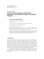
Removal of out-of-band noise and downconversion

Discretization and normalization

Estimation of the first-order CM magnitude at candidate CFs
over the range corresponding to the signal bandwidth
normalized to sampling frequency

Selection of candidate CFs at which estimated first-order CM
magnitudes exceed the cut-off value, Vco

Determination of the number of CFs by applying a
cyclostationarity test to selected candidate CFs

Decision-making based on the number of CFs

FSK signal of modulation order, M, AM signal, or noise or other signals,
such as SSB, DSB, SCLD, and CP-SCLD

Figure 1: Block diagram of the proposed first-order
cyclostationarity-based joint detection and classification algorithm.

4. First-Order Cyclostationarity-Based Joint
Detection and Classification of FSK and
AM Signals
The existence and number of first-order CFs are, respectively,
exploited for the detection and classification of FSK and
AM signals. A first-order cyclostationarity-based joint signal
detection and classification algorithm is proposed, with
relaxed a priori information on the parameters of the
received signal. Furthermore, a benchmark is developed
under the assumption that a priori information on the signal
parameters is available at the receive-side.
4.1. Proposed Algorithm. With the proposed algorithm, the

joint detection and classification of FSK and AM signals
is formulated as a multiple-hypothesis testing problem, as
follows: (i) the received signal is AM if a single first-order
CF is detected; (ii) the received signal is 2-FSK if two firstorder CFs are detected; (iii) the received signal is M-FSK
(M = 2m , M ≥ 4) if the number of first-order CFs which
are detected belongs to the interval [2m−1 + 1, 2m ] (A simple
majority decision criterion is applied here. More complicated
criteria, which can take into account the distance between
CFs can be conceived. Obviously, diverse criteria can lead to
different performance. This will be studied in future work.);
(iv) there is no signal (only noise) or the signal is SSB, DSB,

SCLD, or CP-SCLD, if no first-order CFs are detected. To
further detect and classify the latter signals, second- and
higher-order signal cyclostationarity can be exploited [13–
18].
The proposed algorithm consists of the following two
steps.
Step 1. The magnitude of the first-order CM of the normalized signal is estimated at candidate CFs, α , over a
range corresponding to the bandwidth normalized to the
sampling rate, and based on a K sample observation interval.
According to the theoretical derivations, the first-order CM
magnitude for FSK and AM signals is nonzero only at
CFs given in (11) and (14), respectively, whereas for noise
and another signals this is zero at all CF candidates. Note
that these results are obtained for an infinite observation
interval. When estimation is performed based on a finite
length data sequence (K samples), nonzero values are
attained for the first-order CM magnitude of both FSK
and AM at candidates other than CFs, while such values

are achieved at all CF candidates for noise and the other
signals. Thus, estimates obtained using finite length data
sequences result in the presence of a noise floor. Nevertheless,
these nonzero values are statistically insignificant. On the
other hand, for both FSK and AM signals, the first-order
CM magnitude at CFs decreases with a decrease in SNR,
and thus, below a certain SNR, this becomes comparable
with the nonzero statistically insignificant values. A cutoff
value, Vco , is set, and candidate CFs which correspond to
a CM magnitude above or equal to Vco are selected for
testing in the next step. (Extensive simulations were run to
investigate the values of the noise floor for diverse observation intervals, SNRs, sampling frequencies, and signal
parameters. Based on these results, cutoff values were set
such that most of the statistically insignificant peaks lie
below these values (see Section 6 for details). A rigorous
mathematical analysis of the noise floor distribution, to be
employed for the cutoff value setting, is beyond the scope
of this paper and will be addressed in future work.) By
using (12) and (15), one can obtain the theoretical value
of the SNR for which the first-order CM magnitude at CFs
equals Vco for the M-FSK and AM signals, respectively.
The notation SNRco will be subsequently used for this
SNR. It is noteworthy that for SNRs well above SNRco ,
peaks corresponding to all CFs will be tested, whereas
for SNRs well below SNRco , these will lie below the
cutoff value, Vco , and be missed. Examples are given in
Section 6.
Step 2. The cyclostationarity test developed in [33] is used
to check whether or not the candidate CFs selected in Step 1
of the algorithm are indeed CFs. A detailed description of

this test is provided in Appendix B. A first-order CM-based
statistic is estimated at each candidate CF and compared
against a threshold. The threshold is set from a given
(asymptotic) probability of false alarm. This is defined as the
probability to decide that a candidate CF is a CF when it
is actually not, under the assumption that the observation


EURASIP Journal on Advances in Signal Processing

5
0.2

0.35

0.18
0.3

0.16
0.14
|mr (α )|

(K)

0.2

(K)

|mr (α )|

0.25

0.15

0.12
0.1
0.08
0.06

0.1

0.04
0.05

0.02

0
−0.5 −0.4 −0.3 −0.2 −0.1 0
0.1 0.2 0.3
Candidate cycle frequency, α

0.4

0
−0.5 −0.4 −0.3 −0.2 −0.1

0.3

0.4

0.5

0
−0.5 −0.4 −0.3 −0.2 −0.1 0
0.1 0.2 0.3
Candidate cycle frequency, α

0.5

0.2

0.4

0.5

(b)

0.06

0.035

0.05

0.03
0.025
|mr (α )|

0.04
0.03

0.02

(K)

(K)

0.1

Candidate cycle frequency, α

(a)

|mr (α )|

0

0.015

0.02
0.01
0.01

0.005

0
−0.5 −0.4 −0.3 −0.2 −0.1 0
0.1 0.2 0.3
Candidate cycle frequency, α

0.4

0.5

(c)

(d)

Figure 2: The magnitudes of the first-order estimated CM of the 4-FSK signal, at candidate CFs α , α ∈ [−1/2, 1/2), for (a) 20 dB SNR, (b)
0 dB SNR, (c) −13 dB SNR, and (d) −20 dB SNR.

interval goes to infinity, and is calculated based on the
(asymptotic) chi-squared distribution of the test statistic at
non-CFs. If the estimated statistic at a candidate CF exceeds
the threshold, then the candidate is decided to be a CF. The
number of CFs is finally employed to make a decision on the
signal detection and classification.
The block diagram of the proposed algorithm is shown
in Figure 1. Note that the algorithm requires only minimal a
priori information on the parameters of the signal.
4.2. Proposed Benchmark. The proposed benchmark is developed under the assumption that the first-order CFs of the
signals of interest are known at the receive-side. These CFs
are tested with the aforementioned cyclostationarity test
and the same decision criterion is applied. As such, the

joint detection and classification of FSK and AM signals
is formulated as a multiple hypothesis-testing problem, as
follows: (i) the received signal is AM if corresponding
(known) first-order CF is detected; (ii) the received signal is
2-FSK if the two corresponding (known) first-order CFs are
detected; (iii) the received signal is M-FSK (M = 2m , M ≥ 4)

if at least 2m−1 + 1 out of the M corresponding (known) firstorder CFs are detected; (iv) there is no signal (only noise) or
the signal is SSB, DSB, SCLD, CP-SCLD, if no first-order CF
is detected.

5. Theoretical Performance Analysis
The proposed algorithm involves the steps of finding candidate CFs at which the magnitudes of estimated first-order


6

EURASIP Journal on Advances in Signal Processing
1
0.5

0.9
0.8

0.4

0.6
|mr (α )|

0.5

0.3

(K)

(K)

|mr (α )|

0.7

0.4

0.2

0.3
0.2

0.1

0.1
0
0.1 0.2 0.3
−0.5 −0.4 −0.3 −0.2 −0.1 0
Candidate cycle frequency, α

0.4

0
−0.5 −0.4 −0.3 −0.2 −0.1

0.5

0

0.4

0.5

(b)
0.035

0.03

0.03

0.025

0.025

0.02

0.02

(K)

|mw (α )|

0.035

(K)

0.3

Candidate cycle frequency, α

(a)

|mr (α )|

0.2

0.1

0.015

0.015

0.01

0.01

0.005

0.005

0
−0.5 −0.4 −0.3 −0.2 −0.1 0
0.1 0.2
Candidate cycle frequency, α

0.3

0.4

0.5

0
−0.5 −0.4 −0.3 −0.2 −0.1

0

0.1

0.2

0.3

0.4

0.5

Candidate cycle frequency, α

(c)

(d)

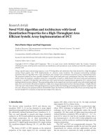
Figure 3: The magnitudes of the first-order estimated CM at candidate CFs α , α ∈ [−1/2, 1/2), for (a) AM, (b) 2-FSK, (c) 2-PSK signals at
20 dB SNR, and (d) noise with power 20 dBm.

CM exceed the cutoff value, applying a cyclostationarity test
to find the number of first-order CFs, and using this result for
decision making. Theoretically, no candidate CFs are tested
for SNRs below SNRco (with infinite length data sequence
and for this SNR range, both statistically significant and
insignificant CM values lie below Vco and are not tested

in Step 2). As a result, the probability of detection and
correct classification for AM and FSK signals equals zero,
(AM
(MFSK
that is, Pdc |AM) = 0 and Pdc |MFSK) = 0 . On the
other hand, theoretically, all CFs and no other candidate
CFs are tested for SNRs above SNRco . Apparently, in this
case, the probability of detection and correct classification
for AM signals equals the probability that the corresponding
CF passes the cyclostationarity test in Step 2 of the algorithm, or, in other words, the probability of detecting the

CF. Furthermore, the probability of detection and correct
classification for 2-FSK and M-FSK (M ≥ 4) signals is given
by the probability of detecting two and between 2m−1 + 1 and
2m CFs, respectively. Given the assumption of independent
detection of CFs, one can show that the expressions for the
(AM
probabilities of detection and correct classification Pdc |AM)
(MFSK|MFSK)
and Pdc
are, respectively, given by

(AM
(1)
Pdc |AM) = Pd ,

(MFSK
Pdc |MFSK)

M

=
ν0 =1

(ν
Pd 0 )

(17)
M/2−1
M ≥4

+
m=1

Pm ,

(18)


EURASIP Journal on Advances in Signal Processing

7
modulating signal, m(t), is obtained by lowpass filtering
a sequence of zero-mean Gaussian random numbers, with
unit variance. The modulation index, μA , is set to 0.3. The
carrier phase, θ, is uniformly distributed over [−π, π), the
carrier frequency offset, Δ f , is equal to 240 Hz, and the time
delay, t0 , is equal to 0.6T and 10 fs−1 for the M-FSK and
AM signals, respectively. The received signals are sampled
at rate fs = 48 kHz, and the cutoff value, Vco , is set to

0.05, unless otherwise mentioned. The threshold Γ used
for CF detection with the cyclostationarity test in Step 2
of the algorithm is set to 15.202, which corresponds to an
(asymptotic) probability of false alarm of 5 × 10−4 [34]. The
probability of detection and correct classification, used as a
performance measure, is estimated from 1000 Monte Carlo
trials.

1

0.95

0.85

Pdc

(2FSK|2FSK)

0.9

0.8

0.75

0.7
0.01 0.02

0.03 0.04

0.05

0.06 0.07
Vco

SNR = −11 dB
SNR = −13 dB

0.08

0.09

0.1

SNR = −15 dB
SNR = −17 dB

Figure 4: The probability of detection and correct classification,
(2FSK
Pdc |2FSK) , as a function of the cutoff value, Vco , for several SNR
values and 1-second observation interval.

where
M

Pm =

ν1 ≥1,...,νm ≥1 νm+1 ∈S(ν1 ,...,νm )
νm >···>ν1
(ν )

× 1 − Pd m

(ν
Pd m+1 )

(19)
(ν )

· · · 1 − Pd 1 ,

S(ν1 ,...,νm ) = {ν : 1 ≤ ν ≤ M, ν = ν1 , . . . , νm },
/

(20)

(ν)
and Pd is the probability of detecting the νth CF (see
Appendix B for details).
As the cutoff value is, theoretically, set above statistically
insignificant peaks, when noise or SSB, DSB, SCLD, or CPSCLD signals are present at the receive-side, no candidate
CFs are selected in Step 1 to be tested in Step 2 of the
algorithm. As such, no first-order CFs are detected, and the
probability of detecting noise or such signals equals one.
Note that this analysis remains valid for the benchmark,
except that (17) and (18) also apply for SNRs below SNRco
(no cutoff value, Vco , is employed with known CFs at the
receive side).

6. Numerical Results and Discussions
6.1. Simulation Setup. M-FSK, M = 2, 4, and 8, and

AM signals with a single-sided bandwidth of 3 kHz and
unit power are simulated. Unless otherwise mentioned,
the observation interval available at the receive-side is 1
second, which is equivalent to 1500 2-FSK symbols, 750 4FSK symbols, and 375 8-FSK symbols, and the frequency
deviation equals T −1 (l = 1). For the AM signal, the

6.2. Simulation Results
6.2.1. Estimated First-Order CM Magnitude. In Figure 2,
the magnitudes of the first-order estimated CM of 4-FSK
signals, |m(K) (α )|, are, respectively, plotted versus candidate
r
CFs, α ∈ [−1/2, 1/2), for several different SNRs. The
peaks in |m(K) (α )| at α = α decrease with SNR, until
r
they become comparable with the statistically insignificant
peaks, which occur at α = α. By using (12), a value of
/
−13.8 dB can be obtained for SNRco . As expected from
the theoretical analysis, the estimated CM magnitude at
CF, α , is around 0.25 at 20 dB SNR (see Figure 2(a)). In
addition, for SNRs well above SNRco , the estimated CM
magnitudes lie above Vco (see Figures 2(a) and 2(b)) for
all M CFs, at SNRs around SNRco , these are near Vco
(see Figure 2(c)), and for SNRs well below SNRco , they
all drop below Vco (see Figure 2(d)). In Figures 3(a)–3(c),
the magnitudes of the first-order estimated CMs of AM, 2FSK, and 2-PSK signals, |m(K) (α )|, are, respectively, plotted
r
versus candidate CFs, α ∈ [−1/2, 1/2), at 20 dB SNR. Results
for noise only, |m(K) (α )|, are presented in Figure 3(d), for
w

20 dBm noise power. One can notice the peaks in |m(K) (α )|
r
of AM and 2-FSK signals at α = α, with magnitudes
around 1 and 0.5, respectively. On the other hand, no such
peaks are seen for 2-PSK and noise, and the magnitude
of the statistically insignificant peaks lie below the cutoff
value.
Further comments can be made regarding the estimation
of the first-order CM magnitudes: (i) this estimation is done
by using (9), which practically represents the discrete Fourier
transform (DFT) of the data sequence; the DFT of the signal
is empirically employed to identify the modulation order
of FSK signals in [10], and a connection with this work
can be inferred; (ii) efficient implementations of the DFT,
specifically the various forms of the fast Fourier transform,
such as those described in [35], can be used to reduce
computational cost. In this paper, the standard CooleyTukey radix-2 decimation in time fast Fourier transform
algorithm is used to calculate K point DFTs, with only the N
points of the resulting K point frequency domain spectrum
corresponding to the signal bandwidth being used. As such,
the computational complexity is of order O(K log K).


8

EURASIP Journal on Advances in Signal Processing

0.96

0.94

0.94

0.92

0.92

(2FSK|2FSK)

0.98

0.96

0.9

Pdc

Pdc

1

0.98

(AM|AM)

1

0.88

0.9

0.88

0.86

0.86

0.84

0.84

0.82

0.82

0.8
−28

0.8
−26

−24

−22

−20

−18

−16

−14

−12

−20 −19 −18 −17

−10

−16 −15 −14 −13 −12 −11 −10

SNR (dB)

SNR (dB)

(a)

(b)

1

1

0.94

0.92

0.92

(8FSK|8FSK)

0.96

0.94

0.9

Pdc

Pdc

0.98

0.96

(4FSK|4FSK)

0.98

0.88

0.9
0.88

0.86

0.86

0.84

0.84

0.82

0.82

0.8

−15

−13

−11

−9

−7

−5

−3

−1

0.8
−10

−9

−8

−7

SNR (dB)
Unknown CFs, theoretical
Unknown CFs, simulations

Known CFs, theoretical
Known CFs, simulations

6.2.2. Setting the Cutoff Value. The cutoff value, Vco , is
empirically set based on the study of the statistically
insignificant peaks for signals of interest, including AM,
M-FSK, M = 2, 4, 8, and noise, for a diverse selection
of signal parameters such as bandwidth and frequency
deviation, sampling frequency, observation interval, and
SNR. Examples of the cutoff values are given in Table 1
for different observation intervals (number of samples).
For these results, the sampling frequency was set to 16
times the bandwidth, and frequency deviation to lT −1 , l =
1, 2, 3. Regardless of the SNR, increasing the observation
interval allows a lower cutoff value, as the CM estimates
are more accurate (asymptotically, the CM magnitudes

−5 −4
SNR (dB)

−3

−2

−1

0

Unknown CFs, theoretical
Unknown CFs, simulations

Known CFs, theoretical
Known CFs, simulations

(c)

Figure 5: The probability of detection and correct classification, (a)
with 1-second observation interval.

−6

(d)
(AM
Pdc |AM) ,

(b)

(2FSK
Pdc |2FSK) ,

(c)

(4FSK
Pdc |4FSK) ,

(8FSK
and (d) Pdc |8FSK) versus SNR,

corresponding to the noise floor go to zero). Figure 4
shows the performance achieved for correctly detecting and
(2FSK
classifying 2-FSK signals, Pdc |2FSK) , as a function of the
cutoff value and for different SNR values. Note that as
the SNR decreases, the performance is severely degraded
by an increase in the cutoff value. This result is expected
since a higher cutoff value leads to a higher SNRco , and,
as the SNR decreases, the statistically significant peaks are
missed in Step 1 of the algorithm. On the other hand,
the performance is only slightly degraded for lower cutoff
values. The SNRco decreases as Vco decreases, and the
statistically significant peaks lie above the cutoff value.
However, statistically insignificant peaks also exceed the


EURASIP Journal on Advances in Signal Processing

9

Table 1: Examples of cutoff values for several observation intervals.
Observation interval
(number of samples ×103 )
36 to 48
48 to 60
60 to 72

96 to 108

Cutoff value, Vco
0.055
0.050
0.045
0.003

1
0.98
0.96

Pdc

(2FSK|2FSK)

0.94
0.92
0.9
0.88
0.86
0.84
0.82
0.8
−23

−21

−19

−17

−15

−13

−11

SNR (dB)
2 s, Vco = 0.03, fd = 1/T
1.25 s, Vco = 0.045, fd = 1/T
1 s, Vco = 0.05, fd = 1/T

1 s, Vco = 0.05, fd = 2/T
1 s, Vco = 0.05, fd = 3/T

Figure 6: The probability of detection and correct signal classifica(2FSK
tion, Pdc |2FSK) , versus SNR, for several observation intervals and
frequency deviations.

be achieved with a lower SNR for AM and lower-order FSK
modulated signals; (ii) the performance differential for the
proposed algorithm and benchmark increases with the FSK
signal modulation order. This behavior is attributed to the
decreased accuracy of the CM estimation resulting from the
decrease in the number of symbols for a given observation
interval available at the receive-side (see Section 6.1 for the
simulation setup). This leads to more CFs being missed
in Step 1 as the SNR decreases, and consequently, to a
degradation of the classification performance in the absence

of a priori knowledge of the CFs; (iii) the simulation
results are very close to the theoretical predictions for the
benchmark over the entire SNR range, whereas this is valid
for the proposed algorithm at SNRs well above SNRco . The
latter behavior is an expected consequence of assuming that
all statistically significant peaks exceed Vco for SNRs above
SNRco in the theoretical performance analysis. As shown in
Figure 2(c), for SNRs close to SNRco , statistically significantly
peaks can be missed in Step 1. Figure 6 presents simulation
results for 2-FSK signal detection and classification for
different observation intervals, obtained by varying the
number of symbols. As expected, improved performance
is obtained with a longer observation interval, since a
lower cutoff value can be set, thus allowing a reduction in
SNRco . In addition, results for different frequency deviations
are shown for a given observation interval. Interestingly,
the results obtained for larger frequency deviations (l =
2, 3) are relatively close to those obtained for l = 1. In
addition, we have simulated scenarios when only noise
or other signals, such as 4-PSK, 16-QAM, 64-QAM, SSB,
and DSB, are present, and have estimated the average
probability for deciding that no FSK and AM signal is
present. For SNRs above −20 dB, this probability is close to
one.

7. Conclusions
cutoff value and are selected to be tested in Step 2 of the
algorithm. Reducing the cutoff value increases the number
of statistically insignificant peaks selected, but most of these
peaks do not pass the cyclostationarity test in Step 2, and

the degradation in performance is not significant. However,
the increase in the number of tested peaks does increase the
computational cost. For the case under study, a cutoff value
of 0.05 is a reasonable choice, as this provides a low SNRco
and minimizes the selection of statistically insignificant peaks
in Step 1 of the algorithm.
6.2.3. Performance of the Proposed Algorithm and Comparison
Against the Benchmark. Performance results obtained from
both theoretical performance analysis and simulations of the
proposed algorithm and benchmark are presented in Figures
(AM
(MFSK
5 and 6, where Pdc |AM) and Pdc |MFSK) are plotted as a
function of SNR. Several conclusions can be inferred: (i) for
the same observation interval, a specified performance can

An algorithm based on first-order cyclostationarity has
been developed for the joint detection and classification of
FSK and AM signals. Theoretical analysis and simulation
experiments demonstrate that the algorithm is able to
discriminate between AM and FSK modulation types with
minimal requirements for a priori information about the
signal parameters. A comparison of these results with a performance benchmark, based on the assumption of additional
a priori signal parameter information being available at
the receive-side, demonstrates that the algorithm performs
reasonably well. Future work will address additional issues
of interest, such as a theoretical analysis of the minimum
length of the observation interval required at the receiveside to attain a specified performance at a given SNR,
the investigation and comparison of diverse methods for
detecting the existence/number of cycle frequencies in the

received signal, the extension to other modulation types, and
more complex propagation environments.


10

EURASIP Journal on Advances in Signal Processing

Appendices

=C

A. First-Order Cyclostationarity of M-FSK and
AM Signals Affected by Gaussian Noise,
Phase, Frequency Offset, and Time Delay
The first-order time-varying moment of the M-FSK signals
is expressed as

(A.1)

e j2π fΔ sm (t−iT −εT) g(t − iT − t0 )e j2πΔ f t ,

m=1 i

√

where it is assumed that A = S. The average is performed
with respect to the unknown data symbols, under the
assumption that the symbol over the ith period takes
equiprobable values in the signal alphabet, AM −FSK .

Equation (A.1) can be further written as
⎛

M

δ(t − iT − t0 )⎠e j2πΔ f t ,

m=1

∞

i

where C = Se jθ M −1 , δ(t) is the Dirac delta function, and
is the convolution operator.
If Δ f = 0, mr (t) is seen to be a periodic function of t,
with fundamental period T [20]. In this case, the first-order
time-varying moment can be easily expressed as a Fourier
series. Such an expression is derived in [20], for t0 = 0 and
g(t) = uT (t). On the other hand, with Δ f = 0, the Fourier
/
transform of (A.2) yields
I mr (t)
⎛

−∞ m=1

⎞

⎝e j2π fΔ sm t g(t) ⊗

δ(t − iT − t0 ) ⎠
i

× e j2πΔ f t e− j2π αt dt
∞

=C

α = Δ f + iT −1 ,

e j2π fΔ sm υ g(υ)

(A.4)

The α-frequency domain is thus seen to be discrete. By
substituting (A.4) into (A.3), we obtain

M

−1

δ α − Δ f − iT −1 e− j2πit0 T T −1

=C
m=1 i
∞
−∞

(A.5)

−1
g(υ)e− j2π ( fΔ sm −iT )υ dυ.

If the product fΔ sm is an integer of T −1 , that is, fΔ sm = pT −1 ,
with p as an integer, then the integral on the right side
of (A.5) equals G((p − i)T −1 ), with G( f ) as the Fourier
transform of g(t). Since the receive filter passes the signal
without attenuation over the effective frequency range, the
nulls of G( f ) will be nearly the same as the frequency nulls of
uT (t). Thus, G((p − i)T −1 ) equals T if p = i and 0 otherwise,
and (A.5) becomes
−1

e− j2π pt0 T δ α − Δ f − pT −1 ,

I mr (t) = C

(A.6)

p∈P

where P = { p : p integer, p = fΔ sm T, sm ∈ AM −FSK }.
If fΔ = lT −1 , with l as an integer, it follows that p =
±l, ±3l, . . . , ±(M − 1)l, and the spectrum consists of M finitestrength additive components,
−1

I mr (t) =
p∈{±l,±3l,...,±(M −1)l}

Ce− j2π pt0 T δ α − Δ f − pT −1 .
(A.7)

δ(t − υ − iT − t0 )e− j2π(α−Δ f )t dυ dt
The expression for mr (t) thus becomes

i

×

i integer.

M

−∞ m=1

×

=C

δ α − Δ f − iT −1 e− j2π(α−Δ f )t0 ,

where I{·} denotes the Fourier transform. Convolution and
change of variables are, respectively, performed at the second
and fourth steps in the right hand-side of (A.3), and the
identity I{ i δ(u − iT)} = T −1 i δ(α − iT −1 ) is used in
the fifth step. Note that I{mr (t)} = 0 if
/

×

M

e j2π fΔ sm υ e− j2π(α−Δ f )υ g(υ)dυ

(A.3)

√

∞

M

−∞ m=1

(A.2)

=C

δ(u − iT)e− j2π(α−Δ f )u du e− j2π(α−Δ f )(υ+t0 ) dυ

−∞ i

I mr (t)

⎞

⎝e j2π fΔ sm t g(t)

mr (t) = C

∞

e j2π fΔ sm υ g(υ)

i

= Se jθ M −1
M

−∞ m=1

×

=C

M

× T −1

mr (t) = E[r(t)]

×

∞

∞

M

−∞ m=1
∞
−∞ i

e j2π fΔ sm υ g(υ)

δ(t − υ − iT − t0 )e− j2π(α−Δ f )t dt dυ

−1
−1
Ce− j2π pt0 T e j2π (Δ f +pT )t . (A.8)

mr (t) =
p∈{±l,±3l,...,±(M −1)l}

This is seen to be equivalent to (5), with κ = {Δ f +
γ, γ = pT −1 , p = ±l, ±3l, . . . , ±(M − 1)l}, and


EURASIP Journal on Advances in Signal Processing
√

11

−1

mr (α) = SM −1 e jθ e− j2π pt0 T . Note that the same expression for the first-order CM at CF α, mr (α), can be
obtained by applying (6). From the results previously
derived for the continuous-time signal, r(t), (10)-(11) can
be obtained for the normalized discrete-time signal, r[k] =

√
r(t)|t=k fs−1 / S + N , by applying (7) and (8), and taking into
account the signal normalization.
With the signal model given in (3), a similar analysis
can be easily performed for AM signal, leading to results
presented in (13) and (14).

B. Cyclostationarity Test and Probability of
CF Detection

(B.1)

is formed, with Re{·} and Im{·} as the real and imaginary
parts, respectively.
(ii)The statistic
−
T (K) = K m(K) Σr 1 m(K)†
r
r

(B.2)

is computed for the candidate CF, α . Here the superscripts
−1 and † denote matrix inverse and transpose, respectively,

and Σr is an estimate of the covariance matrix
⎡

Q2,0 + Q2,1

⎢ Re
2
Σr = ⎢
⎣
Q2,0 + Q2,1

Im

2

(B.4)

Based on the fact that the (asymptotic) distribution of T (K)
under the hypothesis H1 is normal, with mean mT =
2
−
−
Kmr Σr 1 m† and variance σT = 4Kmr Σr 1 m† [33], the
r
r
expression for the (asymptotic) probability of CF detection
is given by
∞

(Γ−mT )/σT

(2π)−1/2 e− y /2 d y.
2

(B.5)

List of Abbreviations
AM:
CF:
CM:
CP-SCLD:
DFT:
DSB:
FB:
FSK:
LB:
PSK:
QAM:
SCLD:
SNR:
SSB:
UHF:
VHF:

Amplitude modulation
Cycle frequency
Cyclic moment
Cyclically prefixed single carrier linear digital
Discrete Fourier transform
Double side-band
Feature-based
Frequency shift keying
Likelihood-based
Phase shift keying
Quadrature amplitude modulation

Single carrier linear digital
Signal-to-noise ratio
Single side-band
Ultra high frequency
Very high frequency.

Acknowledgment
This work has been supported by Defence Research and
Development Canada.

⎤

Q2,0 − Q2,1
⎥
2
⎥
Q2,1 − Q2,0 ⎦,
Re
2

Pd = Pr T (K) ≥ Γ | H1 .

Pd =

A.1. Cyclostationarity Test. With this cyclostationarity test,
the presence of a CF is formulated as a binary hypothesistesting problem; that is, under hypothesis H0 the tested
candidate CF, α , is not a CF, α, and under hypothesis H1
the tested candidate CF, α , is a CF, α. This test is applied here
to first-order candidate CFs (In [33], the test is developed for
real-valued signals. However, it can easily be shown that this

remains valid for complex-valued signals.) and consists of the
following three steps [33].
(i) The first-order CM at candidate CF, α , is estimated
from K samples. The vector
m(K) = Re m(K) (α ) Im m(K) (α )
r
r
r

B.2. Probability of CF Detection. With the previously presented cyclostationarity test, the probability of deciding that
a CF is indeed a CF, which is referred to as the probability of
CF detection, is given as

Im

(B.3)

where covariances Q2,0 and Q2,1 are, respectively,
given
as
limK → ∞ KCum[m(K) (α ), m(K) (α )]
and
r
r
(K)
(K)∗
∗
limK → ∞ KCum[mr (α ), mr (α )], with
as complex
conjugate and Cum[·] as the cumulant operator.

For the estimators of these covariances, see, for example,
(48) in [33].
The statistic T (K) has an (asymptotic) chi-square distribution with two degrees of freedom under the hypothesis H0 ,
whereas an (asymptotic) normal distribution under H1 [33].
(iii)The decision on the candidate CF, α , is made by
comparing the statistic T (K) against a threshold, Γ. This
threshold is set for a specific (asymptotic) probability of false
alarm, defined as Pr{T (K) ≥ Γ | H0 }, under the assumption
that the number of samples goes to infinity, and found from
the tables of the chi-squared distribution. If T (K) ≥ Γ, the
tested candidate is decided to be a CF, otherwise not.

References
[1] J. Mitola III, “Cognitive radio for flexible mobile multimedia
communications,” in Proceedings of the IEEE International
Workshop on Mobile and Multimedia Communications, pp. 3–
10, San Diego, Calif, USA, 1999.
[2] S. Haykin, “Cognitive radio: brain-empowered wireless communications,” IEEE Journal on Selected Areas in Communications, vol. 23, pp. 201–220, 2005.
[3] Federal Communication Commission, “Spectrum policy task
force,” ET Docket No. 02-155, November 2002.
[4] O. A. Dobre, A. Abdi, Y. Bar-Ness, and W. Su, “Survey
of automatic modulation classification techniques: classical
approaches and new trends,” IET Communications, vol. 1, pp.
137–156, 2007.
[5] B. F. Beidas and C. L. Weber, “Higher-order correlation-based
approach to modulation classification of digitally frequencymodulated signals,” IEEE Journal on Selected Areas in Communications, vol. 13, pp. 89–101, 1995.
[6] B. F. Beidas and C. L. Weber, “Asynchronous classification
of MFSK signals using the higher order correlation domain,”

12

[7]

[8]

[9]

[10]

[11]

[12]

[13]

[14]

[15]

[16]

[17]

[18]

[19]

[20]

[21]

EURASIP Journal on Advances in Signal Processing
IEEE Transactions on Communications, vol. 46, no. 4, pp. 480–
493, 1998.
S. Z. Hsue and S. S. Soliman, “Automatic modulation
classification using zero crossing,” IEE Proceedings F, vol. 137,
no. 6, pp. 459–464, 1990.
K. C. Ho, W. Prokopiw, and Y. T. Chan, “Modulation
identification of digital signals by the wavelet transform,” IEE
Proceedings: Radar, Sonar and Navigation, vol. 147, pp. 169–
176, 2000.
A. V. Rosti and V. Koivunen, “Classification of MFSK
modulated signals using the mean of complex envelope,”
in Proceedings of the European Signal Processing Conference
(EUSIPCO ’00), pp. 581–584, 2000.
Z. Yu, Y. Q. Shi, and W. Su, “M-ary frequency shift keying
signal classification based-on discrete Fourier transform,” in
Proceedings of the IEEE Military Communications Conference
(MILCOM ’03), vol. 2, pp. 1167–1172, 2003.
E. E. Azzouz and A. K. Nandi, Automatic Modulation Recognition of Communication Signals, Kluwer Academic Publishers,
Dordrecht, The Netherlands, 1996.
W. A. Gardner, “Signal interception: a unifying theoretical
framework for feature detection,” IEEE Transactions on Communications, vol. 36, pp. 897–906, 1988.
C. M. Spooner, “Classification of cochannel communication
signal using cyclic cumulants,” in Proceedings of the Asilomar
Conference on Signals, Systems and Computers (ASILOMAR
’95), pp. 531–536, 1995.
C. M. Spooner, W. A. Brown, and G. K. Yeung, “Automatic
radio-frequency environment analysis,” in Proceedings of

the Asilomar Conference on Signals, Systems and Computers
(ASILOMAR ’00), vol. 2, pp. 1181–1186, 2000.
O. A. Dobre, Y. Bar-Ness, and W. Su, “Robust QAM
modulation classification algorithm using cyclic cumulants,”
in Proceedings of the IEEE Wireless Communications and
Networking Conference (WCNC ’04), vol. 2, pp. 745–748, 2004.
O. A. Dobre, A. Abdi, Y. Bar-Ness, and W. Su,
“Cyclostationarity-based blind classification of analog
and digital modulations,” in Proceedings of the IEEE Military
Communications Conference (MILCOM ’06), pp. 1–7, 2006.
A. Punchihewa, O. A. Dobre, S. Rajan, and R. Inkol,
“Cyclostationarity-based algorithm for blind recognition of
OFDM and single carrier linear digital modulations,” in
Proceedings of the IEEE International Symposium on Personal,
Indoor and Mobile Radio Communications (PIMRC ’07), pp.
1–5, 2007.
O. A. Dobre, Q. Zhang, S. Rajan, and R. Inkol, “Second-order
cyclostationarity of cyclically prefixed single carrier linear
digital modulations with applications to signal recognition,” in
Proceedings of the IEEE Global Telecommunications Conference
(GLOBECOM ’08), pp. 3513–3517, 2008.
F. Gini and G. B. Giannakis, “Frequency offset and symbol
timing recovery in flat-fading channels: a cyclostationary
approach,” IEEE Transactions on Communications, vol. 46, pp.
400–411, 1998.
A. Ferr´ ol, P. Chevalier, and L. Albera, “Second-order blind
e
separation of first- and second-order cyclostationary sourcesapplication to AM, FSK, CPFSK, and deterministic sources,”
IEEE Transactions on Signal Processing, vol. 52, pp. 845–861,
2004.

M. Shi, Y. Bar-Ness, and W. Su, “Blind OFDM systems parameters estimation for software defined radio,” in Proceedings of
the 2nd IEEE International Symposium on New Frontiers in
Dynamic Spectrum Access Networks (DySpan ’07), pp. 119–122,
2007.

[22] H. Li, Y. Bar-Ness, A. Abdi, O. S. Somekh, and W. Su,
“OFDM modulation classification and parameters extraction,”
in Proceedings of the 1st International Conference on Cognitive Radio Oriented Wireless Networks and Communications
(CROWNCOM ’06), pp. 1–6, 2006.
[23] K. Kim, C. M. Spooner, I. Akbar, and J. H. Reed, “Specific
emitter identification for cognitive radio with application to
IEEE 802.11,” in Proceedings of the IEEE Global Telecommunications Conference (GLOBECOM ’08), pp. 2099–2103, 2008.
[24] K. Kim, I. A. Akbar, K. K. Bae, J. S. Um, C. M. Spooner, and
J. H. Reed, “Cyclostationary approaches to signal detection
and classification in cognitive radio,” in Proceedings of the 2nd
IEEE International Symposium on New Frontiers in Dynamic
Spectrum Access Networks (DySpan ’07), pp. 212–215, 2007.
[25] M. Oner and F. Jondral, “On the extraction of the channel
allocation information in spectrum pooling systems,” IEEE
Journal on Selected Areas in Communications, vol. 25, no. 3, pp.
558–565, 2007.
[26] A. Tkachenko, D. Cabric, and R. W. Brodersen, “Cyclostationary feature detector experiments using reconfigurable BEE2,”
in Proceedings of the 2nd IEEE International Symposium on New
Frontiers in Dynamic Spectrum Access Networks (DySpan ’07),
pp. 216–219, 2007.
[27] O. A. Dobre, S. Rajan, and R. Inkol, “A novel algorithm for
blind recognition of M-ary frequency shift keying modulation,” in Proceedings of the IEEE Wireless Communications and
Networking Conference (WCNC ’07), pp. 521–525, 2007.
[28] O. A. Dobre, S. Rajan, and R. Inkol, “Exploitation of firstorder cyclostationarity for joint signal detection and classification in cognitive radio,” in Proceedings of the IEEE Vehicular
Technology Conference (VTC ’08), pp. 1–5, 2008.

[29] A. B. Carlson, P. B. Crilly, and J. C. Rutledge, Communication
Systems, McGraw Hill, New York, NY, USA, 4th edition, 2002.
[30] W. A. Gardner, Cyclostationarity in Communications and
Signal Processing, IEEE Press, New York, NY, USA, 1994.
[31] A. Napolitano, “Cyclic higher-order statistics: input/output
relations for discrete- and continuous-time MIMO linear
almost-periodically time-variant systems,” Signal Processing,
vol. 42, pp. 147–166, 1995.
[32] A. V. Dandawate and G. B. Giannakis, “Asymptotic theory
of mixed time averages and kth-order cyclic-moment and
cumulant statistics,” IEEE Transactions on Information Theory,
vol. 41, pp. 216–232, 1995.
[33] A. V. Dandawate and G. B. Giannakis, “Statistical tests for
presence of cyclostationarity,” IEEE Transactions on Signal
Processing, vol. 42, pp. 2355–2369, 1994.
[34] M. Abramowitz and I. A. Stegun, Handbook of Mathematical
Functions, Dover Publications, New York, NY, USA, 1972.
[35] C. Van Loan, Computational Framework for the Fast Fourier
Transform, SIAM, Philadelphia, PA, USA, 1992.