Báo cáo hóa học: " Research Article Opportunistic Spectrum Access in Self-Similar Primary Traffic" docx

Hindawi Publishing Corporation
EURASIP Journal on Advances in Signal Processing
Volume 2009, Article ID 762547, 8 pages
doi:10.1155/2009/762547
Research Article
Opportunistic Spectrum Access in Self-Similar Primary Traffic
Xiang y ang Xiao, Keqin Liu, and Qing Zhao
Department of Electrical and Computer Engineering, University of California, Davis, CA 95616, USA
Correspondence should be addressed to Qing Zhao,
Received 16 February 2009; Revised 17 June 2009; Accepted 14 July 2009
Recommended by Ananthram Swami
We take a stochastic optimization approach to opportunity tracking and access in self-similar pr imary traffic. Based on a multiple
time-scale hierarchical Markovian model, we formulate opportunity tracking and access in self-similar primary traffic as a Partially
Observable Markov Decision Process. We show that for independent and stochastically identical channels under certain conditions,
the myopic sensing policy has a simple round-robin structure that obviates the need to know the channel parameters; thus it
is robust to channel model mismatch and variations. Furthermore, the myopic policy achieves comparable performance as the
optimal policy that requires exponential complexity and assumes full knowledge of the channel model.
Copyright © 2009 Xiangyang Xiao et al. This is an open access article distributed under the Creative Commons Attribution
License, which permits unrestricted use, distribution, and reproduction in any medium, provided the original work is properly
cited.
1. Introduction
1.1. Opportunistic Spectrum Access. The “spectrum paradox”
is by now widely recognized. On the one hand, the projected
spectrum need for wireless devices and services continues
to grow, and virtually all usable radio frequencies have
already been allocated. Such an imbalance in supply and
demand threatens one of the most explosive economic and
technological growths in the past decades. On the other
hand, extensive measurements conducted in the recent years
reveal that much of the prized spectrum lies unused at
any given time and location [1]. For example, in a recent

measurement study of wireless LAN traffic[2], a typical
active FTP session has about 75% idle time, and voice-over-
IP applications such as Skype have up to 90% idle time.
These measurements of actual spectrum usage highlight
the drawbacks of the current static spectrum allotment policy
that is at the root of this spectrum paradox. They also
form the key rationale for Opportunistic Spectrum Access
(OSA) envisioned by the DARPA XG program and currently
being considered by the FCC [3]. The idea of OSA is to
exploit instantaneous spectrum opportunities by opening
the licensed spectrum to secondary users. This would allow
secondary users to identify available spectrum resources
and communicate nonintrusively by limiting interference to
primary users. Even for unlicensed bands, OSA may be of
considerable value for spectrum efficiency by adopting a
hierarchical pricing structure to support both subscribers
and opportunistic users.
1.2. Opportunistic Spectrum Access in Self-Similar Primary
Traffic. Since the seminal work of Leland et al. [4], exten-
sive studies have shown that self-similarity manifests in
communications traffic in diverse contexts, from local area
networks to wide area networks, from wired to wireless
applications [5–8]. In this paper, we consider opportunistic
spectrum access in self-similar primary traffic processes with
long-range dependency. We adopt a multiple time-scale
hierarchical Markovian model for self-similar trafficpro-
cesses proposed in [9, 10]. A decision theoretic framework
is developed based on the theory of Partially Observable
Markov Decision Processes (POMDPs).
Unfortunately, solving a general POMDP is often

intractable due to the exponential complexity. A simple
approach is to implement the myopic policy, which only
focuses on maximizing the immediate reward and ignores
the impact of current action on the future reward. We show
in this paper that the myopic policy has a simple and robust
structure under certain conditions. This simple structure
obviates the need to know the transition probabilities of the
underlying multiple time-scale Markovian model and allows
automatic tracking of variations in the primary trafficmodel.
Compared to Markovian channel models, the model at hand
2 EURASIP Journal on Advances in Signal Processing
is more general but requires more parameters, it is thus more
important to have policies that are robust to model mismatch
and parameter variations. The strong performance of the
myopic policy with such a simple and robust structure is
demonstrated through simulation examples.
1.3. Related Work. This paper is perhaps the first that
addresses OSA in self-similar primary traffic. It builds upon
our prior work on a POMDP framework for the joint
design of opportunistic spectrum access that adopts a first-
order Markovian model for the primary traffic. Specifically,
in [11–13], a decision-theoretic framework for tracking
and exploiting spectrum opportunities is developed using
a first-order Markovian model for the primary traffic. A
fundamental result on the principle of separation for OSA
[14, 15] and structural opportunity tracking polices [16, 17]
have been established, leading to simple, robust, and optimal
solutions.
The first-order Markovian model of the primary traffic,
however, has its limitations. It cannot capture the long-range

dependency exhibited in a wide range of communications
traffic. In this paper, we extend the decision-theoretic
framework developed in [11, 12, 14, 15] to incorporate self-
similar primary traffic with long-range dependency. We show
that the structure and optimality of the myopic sensing
policy established in [16, 17] under a first-order Markovian
model are preserved under certain conditions in self-similar
primary traffic modeled by a multiple time-scale hierarchical
Markovian process.
2. A Multiple Time-Scale Hierarchical
Markovian Model for Self-Similar Traffic
A fundamental property of a self-similar process is the “scale-
invariant behavior.” The process is stochastically unchanged
when it is zoomed out by stretching the time domain [18].
Specifically,
{X(t):t ∈ R} is a self-similar process if for any
k
≥ 1, t
1
, , t
k
∈ R,anda, H ∈ R
+
,
(
X
(
at
1
)

, , X
(
at
k
))
d
=

a
H
X
(
t
1
)
, , a
H
X
(
t
k
)

,(1)
where
d
= represents equivalence in distribution. It has been
shown that for 1/2 <H<1, the autocorrelation of a self-
similarly process decreases to zero polynomially, leading to a
long-range dependency behavior.

Based on traffic traces from physical networks, sev-
eral models for self-similar traffic have been developed,
among which is a multiple time-scale hierarchical Markovian
model proposed in [9, 10]. Under this model, trafficis
an aggregation of hierarchical Markovian on-off processes
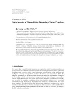
with disparate time-scales. Illustrated in Figure 1 is a two-
level hierarchical on-off process. The higher level process
has a much slower t ransition rate than the lower one. The
resulting t raffic process is “on” (busy) when both Markovian
processes are in state 0 and “off ” (idle) otherwise. This
hierarchical model with two to three levels has been shown to
approximate a self-similar process and fit well with measured
traffic traces. It is motivated by the physical process of traffic
Slow scale
Fast scale
Busy IdleIdleIdle
0
1
0
1
0
1
Figure 1: A multiple time-scale hierarchical Markovian model for
self-similar primary traffic.
generation [9, 10]. Specifically, for a packet to appear in
the physical channel, several events at different time scales
have to occur, including, for example, establishing a session,
releasing a message to the network by a transport protocol
like TCP, then releasing a packet to the channel by the MAC
and physical layers [9, 10].

This hierarchical on-off process can be described by a
Markov process w ith augmented state. For example, the
above two-level hierarchical on-off process can be treated as
a Markov process with 4 states. The resulting trafficmodel
is thus a hidden Markov model: the state (0, 0) is directly
observable and mapped to “on,” and the remaining 3 states
are mapped to a single state “off.” This hidden Markovian
interpretation is the key to our POMDP formulation of
opportunity tracking and exploitation in self-similar pri-
mary traffic as shown in the next section.
3. A POMDP Framework
In this section, we show that under the multiple time-scale
hierarchical Markovian model, opportunity tracking can still
be formulated as a POMDP similar to that developed in [11–
15] under a first-order Markovian model.
3.1. Network Model. Consider a spectrum consisting of N
channels, each with transmission rate B
n
(n = 1, , N).
These N channels are allocated to a primary network with
slotted transmissions. The primary traffic in each channel is
a self-similar process following the hierarchical Markovian
model with L levels. Each channel can thus be represented
by an augmented Markov chain with 2
L
states (see Figure 1
above where L
= 2). The availability (idle or busy) of a
channel, that is, the primary traffic trace, is determined by
the state of the corresponding augmented Markov chain.

Let
{p
(n,k)
ij
}
i, j=0,1
denote the transition probabilities of the
kth (1
≤ k ≤ L) level Markov process for channel n.Wethus
have p
(n,k)
ii
 p
(n,k+1)
ii
and p
(n,k)
ij
 p
(n,k+1)
ij
for i
/
= j,where
1
≤ k ≤ L − 1. In other words, the kth level Markov process
varies much slower than the mth level Markov process for
m>k. It can be shown that the kth le vel Markov process
for channel n is positively correlated when p
(n,k)

11
>p
(n,k)
01
,
and negatively correlated when p
(n,k)
11
<p
(n,k)
01
. We notice that
the Markov processes at higher levels (i.e., with smaller level
EURASIP Journal on Advances in Signal Processing 3
indexes) can be considered as positively correlated due to
their slow transition rates.
Consider next a pair of secondary transmitter and
receiver seeking spectrum opportunities in these N channels.
In each slot, they choose a channel to sense. If the channel is
idle, the transmitter sends packages to the receiver through
this channel, and a reward R(t) is accrued in this slot
(i.e., the number of bits delivered). It is straight forward
to generalize the POMDP framework and the results in
Section 4 to multichannel sensing scenarios. We assume here
that the secondary user has reliable detection of the channel
availability.
Our goal is to develop the optimal sensing policy to
maximize the throughput of the secondar y user during a
desired period of T slots.
3.2. POMDP Formulation. The sequential decision-making

process described above can be modeled as a POMDP.
Specifically, the underlying system state is given by the
state of the augmented Markov chain at the beginning of each
slot. Let S
n
(t) = (S
(1)
n
(t), S
(2)
n
(t), , S
(L)
n
(t)) denote the state
of channel n in slot t,whereS
(k)
n
(t) ∈{0, 1} represents the
state of the kth level Markov process for channel n in slot t.
The transition probabilities of this augmented Markov chain
can be easily obtained from
{p
(n,k)
ij
}
i, j=0,1
(1 ≤ k ≤ L). Let
O
n

(t) ∈{0, 1} denote the availability of channel n in slot t,
that is, O
n
(t) = 0 (busy) when S
(k)
n
(t) = 0forall1≤ k ≤ L
and O
n
(t) = 1 (idle/opportunity) otherwise.
The reward in each slot is the number of bits that can be
delivered by the secondary user. Given sensing action a(t),
the immediate reward R
a(t)
(t)isgivenby
R
a
(
t
)
(
t
)
= O
a
(
t
)
(
t

)
B
a
(
t
)
. (2)
Due to the hidden Markovian model of channel avail-
ability and partial sensing, the state S
n
(t) of the augmented
Markov chain representing each channel cannot be fully
observed. The statistical information on S
n
(t)provided
by the entire decision and observation history can be
encapsulated in a belief vector Λ
n
(t) ={λ
(n,s)
(t):s =
{
s
k
}
L
k
=1
∈{0, 1}
L

},where
λ
(
n,s
)
(
t
)
= Pr

S
n
(
t
)
= s |

a
(
i
)
, O
a
(
i
)
(
i
)


t−1
i
=1

(3)
represents the conditional probability (given the decision
and observation history) that the state of channel n is s in
slot t. The whole system state is given by the concatenation
of each channel’s belief vector:
Λ
(
t
)
=
[
Λ
1
(
t
)
, Λ
2
(
t
)
, , Λ
N
(
t
)

]
.
(4)
This system belief vector Λ(t)isasufficient statistic for
making the optimal action in each slot t. Furthermore, Λ(t +
1) for slot t + 1 can be obtained from Λ(t), a(t), and O
(a(t))
(t)
via Bayes rule as shown in what follows. Let q
(n)
s

s
(s

, s ∈
{
0, 1}
L
) denote the transition probability from state s

to s
for channel n,itiseasytoseethatq
(n)
s

s
=

L

k=1
p
(n,k)
s

k
s
k
.Define
s
0
Δ
={s
k
: s
k
= 0}
L
k
=1
and
λ

(n,s)
(
t
)
Δ
=
⎧

⎪
⎨
⎪
⎩
λ
(n,s)
(
t
)
1 − λ
(n,s
0
)
(
t
)
,ifs
/
= s
0
,
0, if s
= s
0
.
(5)
We then have
λ
(n,s)
(

t +1
)
=
⎧
⎪
⎪
⎪
⎪
⎪
⎪
⎪
⎪
⎪
⎨
⎪
⎪
⎪
⎪
⎪
⎪
⎪
⎪
⎪
⎩

s

∈{0,1}
L
λ


(n,s

)
(
t
)
q
(n)
(s

s)
, a
(
t
)
= n, O
n
(
t
)
= 1,
q
(n)
(s
0
,s)
, a
(
t

)
= n, O
n
(
t
)
= 0,

s

∈{0,1}
L
λ
(n,s

)
(
t
)
q
(n)
(s

s)
, a
(
t
)
/
= n.

(6)
Let π
={π
t
}
T
t
=1
be a series of mappings from Λ(t)toa(t)for
each 1
≤ t ≤ T, which denotes the sensing policy for channel
selection. We then arrive at the following stochastic control
problem:
π
∗
= arg max
π
E
π
⎡
⎣
T

t=1
R
π
t
(Λ(t))
(
t

)
| Λ
(
1
)
⎤
⎦
,(7)
where
E
π
represents the expectation given that the sensing
policy π is employed, π
t
(Λ(t)) is the sensing action in slot t
under policy π,andΛ(1) is the initial belief vector. When
no information is available to the secondary user at the
beginning of the first slot, Λ(1) is given by the stationary
distributions of the on-off Markov processes at all levels of
these N channels. Specifically, λ
(n,s)
(1) is given by
λ
(
n,s
)
(
1
)
=

L

k=1
⎛
⎝
s
k
p
(
n,k
)
01
p
(
n,k
)
01
+ p
(
n,k
)
10
+
(
1 − s
k
)
p
(
n,k

)
10
p
(
n,k
)
01
+ p
(
n,k
)
10
⎞
⎠
.
(8)
4. The Myopic Policy and
Its Semiuniversal Structure
The myopic policy ignores the impact of the cur rent action
on the future reward, focusing solely on maximizing the
expected immediate reward
E[R
a(t)
(t)]. The myopic action
a(t) in slot t given current belief vector Λ(t)isthusgivenby
a
(
t
)
= arg max

a=1, ,N
Pr
[
O
a
(
t
)
= 1 | Λ
(
t
)
]
B
a
= arg max
a=1, ,N

1 − λ
(a,s
0
)
(
t
)

B
a
.
(9)

In general, obtaining the myopic action in each slot
requires the recursive update of the belief vector Λ(t)as
given in (6). Next we show that under certain conditions,
the myopic policy for stochastically identical channels has a
semiuniversal structure that does not need the update of the
belief vector or the knowledge of the transition probabilities.
4 EURASIP Journal on Advances in Signal Processing
Consider stochastically identical channels. Let
{p
(k)
ij
}
i, j=0,1
denote the transition probabilities of the kth
level Markov process for all channels, B the transmission
rate of all channels.
We establish a simple and robust structure of the myopic
policy under certain conditions as shown in Theorem 1.Let
ω
(k)
n
(t) denote the marginal probability that the state of the
kth level Markov process for channel n is 1 in slot t,itis
easy to see that ω
(k)
n
(t) =

s:s
k

=1
λ
(n,s)
(t). We assume that the
initial states are independent across all levels, that is, for all
s
∈{0, 1}
L
λ
(
n,s
)
(
1
)
=

k

s
k
ω
(
k
)
n
(
1
)
+

(
1
− s
k
)

1 − ω
(
k
)
n
(
1
)

.
(10)
Theorem 1. Suppose that channels are independent and
stochastically identical, the Markov processes at all levels are
positively correlated, and the initial states of the Markov
processes are inde pendent across all levels for each channel.
Furthermore, the initial sy stem belief vector Λ(1) satisfies
the following condition. There exists a channel ordering
(n
1
, n
2
, , n
N
) such that ω

(k)
n
1
(1) ≥ ω
(k)
n
2
(1) ≥ ··· ≥ ω
(k)
n
N
(1)
for all 1
≤ k ≤ L, that is, the channel ordering by the
initial states at all levels is the same. The myopic policy has a
round robin structure based on the c ircular channel ordering
(n
1
, n
2
, , n
N
). Starting from sensing channel n
1
in slot 1,the
myopic action is to stay in the same channel when it is idle and
sw itch to the next channel in the circular ordering when it is
busy.
Proof. Without loss of generality, we assume B
= 1. We first

prove the following three lemmas.
Lemma 1. If the states of the Markov processes are independent
(conditioned on the past observations) across all levels for
each channel in slot t, and there exists a channel ordering
(n
1
, n
2
, , n
N
) such that ω
(k)
n
1
(t) ≥ ω
(k)
n
2
(t) ≥ ··· ≥ ω
(k)
n
N
(t)
for all 1 ≤ k ≤ L, then for all t

>t, ω
(k)
n
1
(t


) ≥ ω
(k)
n
2
(t

) ≥
··· ≥
ω
(k)
n
N
(t

) for all 1 ≤ k ≤ L when no observation is made
from t up to t

.
Proof. Starting from slot t, the independence of the states of
the Markov processes (conditioned on the past observations)
acrossalllevelsforeachchannelwillholdaslongasno
observation is made. For any channel n,wehave,forall
1
≤ k ≤ L,
ω
(
k
)
n

(
t

)
=

p
(k,t

−t)
11
− p
(k,t

−t)
01

ω
(k)
n
(
t
)
+ p
(k,t

−t)
01
, (11)
where p

(k,m)
ij
is the m-step transition probability from state i
to j at the kth level. In particular, we have
p
(k,m)
01
=
p
(k)
01
− p
(
k
)
01

p
(
k
)
11
− p
(
k
)
01

m
p

(k)
01
+ p
(k)
10
,
p
(k,m)
11
=
p
(k)
01
+ p
(k)
10

p
(
k
)
11
− p
(
k
)
01

m
p

(k)
01
+ p
(k)
10
.
(12)
Since p
(k)
11
≥ p
(k)
01
,wehavep
(k,m)
11
≥ p
(k,m)
01
for any m ∈ Z
+
.
Consider two channels a and b with ω
(k)
a
(t) ≥ ω
(k)
b
(t). From
(11), it is easy to see that ω

(k)
a
(t

) ≥ ω
(k)
b
(t

)foranyt

>t.
Lemma 1 thus holds.
Lemma 2. If the states of the Markov processes are independent
(conditioned on the past observations) across all levels for each
channel in slot t and the chosen channel n is observed in state
0, then channel n will have the smallest probability ω
(k)
n
(t +1)
of being in state 1 at level k for all 1
≤ k ≤ L in slot t +1.
Proof. Given observation O
n
(t) = 0 in slot t,wehaveω
(k)
n
(t +
1)
= p

(k)
01
for all 1 ≤ k ≤ L.From(11), p
k
01
is the smallest
belief value at level k among all channels in slot t +1.
Lemma 3. Consider channel n with current belief Λ
n
(t) in slot
t.Fort

>t,letλ
(k)
n,s
0
(t

)(0≤ k ≤ t

− t) denote the belief value
in slot t

if k1s are successively observed from slot t to t + k − 1.
One has
λ
(
t

−t

)
n,s
0
(
t

)
≤ λ
(
0
)
n,s
0
(
t

)
.
(13)
Proof. From (12), we have
p
(k, j)
11
≥ p
(k, j)
01
,
p
(k, j)
00

≥ p
(k, j)
10
.
(14)
Let q
( j)
(s,s)
denote the j-step transition probability from
channel state s to s

.From(14), it is easy to see that q
( j)
(s,s)
≥
q
( j)
(s
,s)
for all s, s

∈{0, 1}
L
.Wethushave
λ
(
k
)
n,s
0

(
t

)
=

s∈{0,1}
L
,s
/
= s
0
λ
(k−1)
(n,s)
(
t + k
− 1
)
1 − λ
(k−1)
(n,s
0
)
(
t + k
− 1
)
q
(t


−t−k+1)
(s,s
0
)
≤

s∈{0,1}
L
,s
/
= s
0
λ
(k−1)
(n,s)
(
t + k
− 1
)
q
(t

−t−k+1)
(s,s
0
)
+ q
(
t


−t−k+1
)
(
s
0
,s
0
)
λ
(
k
−1
)
(
n,s
0
)
(
t + k
− 1
)
×

s∈{0,1}
L
,s
/
= s
0

λ
(k−1)
(n,s)
(
t + k
− 1
)
1 − λ
(k−1)
(n,s
0
)
(
t + k
− 1
)
=

s∈{0,1}
L
,s
/
= s
0
λ
(k−1)
(n,s)
(
t + k
− 1

)
q
(t

−t−k+1)
(s,s
0
)
+ λ
(k−1)
(n,s
0
)
(
t + k
− 1
)
q
(t

−t−k+1)
(s
0
,s
0
)
=

s∈{0,1}
L

λ
(k−1)
(n,s)
(
t + k
− 1
)
q
(t

−t−k+1)
(s,s
0
)
= λ
(
k
−1
)
n,s
0
(
t

)
.
(15)
We thus have λ
(t


−t)
n,s
0
(t

) ≤ λ
(t

−t−1)
n,s
0
(t

) ≤··· ≤λ
(0)
n,s
0
(t

).
We are now ready to prove the theorem. Assume
we observed 0 on channel n
1
in slot 1. Based on the
independence of the initial states of the Markov processes
across all levels for each channel, channel n
1
will have the
smallest probability of being idle in the next slot according
EURASIP Journal on Advances in Signal Processing 5

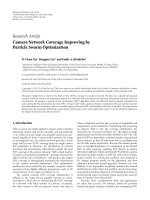
Ch 3
Ch 2
Ch 1
When observe 0
When observe 0 When observe 0
Figure 2: The round robin structure of the myopic policy (N = 3).
to Lemma 2. Furthermore, the order of the probabilities of
being in state 1 at each level for all unobserved channels
will be the same according to Lemma 1, and channel n
1
will have the smallest probability of being in state 1 at each
level. The independence of the states (conditioned on the
past observations) and ordering conditions on the initial
system belief vector still hold in the next slot with channel
ordering (n
2
, , n
N
, n
1
). On the other hand, if we observe
1 on channel n
1
in slot 1, channel n
1
will have the largest
probabilities of b eing idle as long as the observations are
1 on this channel according to Lemmas 3 and 1. When
a 0 is observed after the 1s, channel n
1

will again have
the smallest probability of being in state 1 at each level.
The independence of the states (conditioned on the past
observations) and ordering conditions on the initial system
belief vector still hold in the next slot with channel ordering
(n
2
, , n
N
, n
1
). By induction, it is easy to see that the myopic
policy has a round robin structure with circular ordering
(n
1
, n
2
, , n
N
).
Figure 2 shows an example of the round robin structure
of the myopic policy when N
= 3 with a circular channel
order of (1, 2, 3). The myopic action is to sense the three
channels in turn with random switching times (when the
currentchannelisbusy).
In practice, the channel ordering assumption on the
initial system belief vector in Theorem 1 means that at the
beginning if one level of a channel (say channel m)ismore
likely to be idle than the same level of another channel (say

channel n), then every level of channel m is more likely to
be idle than the same level of channel n. For example, in
the first slot, if it is less likely to have a session established
over channel m than over channel n, then a message is less
likely to be released by a primary user over channel m than
over channel n. If the initial channel ordering assumption
is not satisfied, then before all channels have been visited,
the myopic policy may not have the round-robin structure.
However, after all channels have been visited, the channel
ordering assumption will be satisfied and the structure of the
myopic policy will hold thereafter.
We notice that the secondary user usually has no initial
information about the channel availability. In this case,
the initial system belief vector is given by the stationary
distributions of the underlying Markov processes as given in
(8). The channel ordering assumption on the initial system
belief vector in Theorem 1 is thus satisfied since stochastically
identical channels have the same stationary distribution at
the same level. The circular channel ordering in the round-
robin structure can be set arbitrarily.
For two-level hierarchical Markovian channel models
(L
= 2), we can relax the condition on the initial system
belief vector in Theorem 1 without affecting the round robin
structure of the myopic policy.
Theorem 2 (relaxation of initial condition). Suppose that
channels are independent and stochastically identical, the
Markov processes at all levels are positively correlated, and the
initial states of the Markov processes are independent across all
levels for each channel. The round robin structure of the myopic

policy given in Theorem 1 remains unchanged when for any
two channels i and j with ω
(1)
i
(1) ≥ ω
(1)
j
(1),thefollowingtwo
equations hold:
2

k=1

1 − ω
(k)
i
(
1
)

≤
2

k=1

1 − ω
(k)
j
(
1

)

,
ω
(
2
)
i
(
1
)
− ω
(
2
)
j
(
1
)
≥−

1 − p
(2)
11

p
(1)
11
− p
(1)

01

ω
(1)
i
(
1
)
− ω
(1)
j
(
1
)


1 − p
(1)
11

p
(2)
11
− p
(2)
01

.
(16)
Proof. The proof follows a similar process to Theorem 1.We

first prove the following lemma.
Lemma 4. If the states of the Markov processes are independent
(conditioned on the past observations) across all levels for
each channel in slot t, and there exists a channel ordering
(n
1
, n
2
, , n
N
) such that ω
(1)
n
1
(t) ≥ ω
(1)
n
2
(t) ≥ ··· ≥ ω
(1)
n
N
(t)
and for any 1
≤ i<j≤ N,
2

k=1

1 − ω

(k)
n
i
(
t
)

≤
2

k=1

1 − ω
(k)
n
j
(
t
)

,
(17)
ω
(
2
)
n
i
(
t

)
− ω
(
2
)
n
j
(
t
)
≥−

1 − p
(2)
11

p
(1)
11
− p
(1)
01

ω
(1)
n
i
(
t
)

− ω
(1)
n
j
(
t
)


1 − p
(1)
11

p
(2)
11
− p
(2)
01

.
(18)
One then has for all t

>tunder the condition that no
observation is made from t to t

, (17) and (18) still hold if t
is replaced by t


,andλ
n
1
,s
0
(t

) ≤ λ
n
2
,s
0
(t

) ≤··· ≤λ
n
N
,s
0
(t

).
Proof. By induction, we only need to prove the lemma for
t

= t+1. Since no observation is made from t to t+1, we have
that the states of the Markov processes for each channel are
independent from t to t + 1. We thus have that the expected
immediate reward f (ω
(1)

n
(k), ω
(2)
n
(k)) for channel n at time
k(t
≤ k ≤ t +1)isgivenby
f

ω
(1)
n
(
k
)
, ω
(2)
n
(
k
)

=
1 − λ
n,s
0
(
k
)
= 1 −


1 − ω
(1)
n
(
k
)

1 − ω
(2)
n
(
k
)

.
(19)
Assume that for channel i and j,wehave f (ω
(1)
j
(t), ω
(2)
j
(t)) ≥
f (ω
(1)
i
(t), ω
(2)
i

(t)). Define Δ
(k)
Δ
= p
(k)
11
− p
(k)
01
for k = 1, 2. We
6 EURASIP Journal on Advances in Signal Processing
then have Δ
(1)
≥ Δ
(2)
> 0, ω
(1)
j
(t) ≥ ω
(1)
i
(t), ω
(k)
n
(t +1)=
Δ
(k)
ω
(k)
n

(t)+p
(k)
01
,and
ω
(
2
)
j
(
t
)
− ω
(
2
)
i
(
t
)
≥−

1 − p
(
2
)
11

Δ
(

1
)

ω
(
1
)
j
(
t
)
− ω
1
i
(
t
)
− ω
(
1
)
i
(
t
)


1 − p
(1)
11


Δ
(2)
⇐⇒

1 − p
(
1
)
11

Δ
(
2
)

2

ω
(
2
)
j
(
t
)
− ω
(
2
)

i
(
t
)

+

1 − p
(
2
)
11

Δ
(
1
)

Δ
(
2
)

ω
(
1
)
j
(
t

)
− ω
(
1
)
i
(
t
)

≥
0
=⇒

1 − p
(
1
)
11

Δ
(
2
)

2

ω
(
2

)
j
(
t
)
− ω
(
2
)
i
(
t
)

+

1 − P
(
2
)
11

Δ
(
1
)

2

ω

(
1
)
j
(
t
)
− ω
(
1
)
i
(
t
)

≥
0
=⇒

1 − p
(
1
)
11

Δ
(
2
)


ω
(
2
)
j
(
t +1
)
− ω
(
2
)
i
(
t +1
)

+

1 − p
(
2
)
11

Δ
(
1
)


ω
(
1
)
j
(
t +1
)
− ω
(
1
)
i
(
t +1
)

≥
0.
(20)
We thus proved that (18) still holds if t is replaced by t +1.
From (20)and f (ω
(1)
j
(t), ω
(2)
j
(t)) ≥ f (ω
(1)

i
(t), ω
(2)
i
(t)),
we ha ve

1 − p
(
1
)
11

Δ
(
2
)

ω
(
2
)
j
(
t
)
− ω
(
2
)

i
(
t
)

+

1 − p
(
2
)
11

Δ
(
1
)

ω
(
1
)
j
(
t
)
− ω
(
1
)

i
(
t
)

+ Δ
(
1
)
Δ
(
2
)

f

ω
(
1
)
j
(
t
)
, ω
(
2
)
j
(

t
)

−
f

ω
(
1
)
i
(
t
)
, ω
(
2
)
i
(
t
)

≥
0
⇐⇒

1 − p
(
1

)
11

Δ
(
2
)

ω
(
2
)
j
(
t
)
− ω
(
2
)
i
(
t
)

+

1 − p
(2)
11


Δ
(1)

ω
(1)
j
(
t
)
− ω
(1)
i
(
t
)

+ Δ
(
1
)
Δ
(
2
)

ω
(
1
)

j
(
t
)
+ ω
(
2
)
j
(
t
)
− ω
(
1
)
j
(
t
)
ω
(
2
)
j
(
t
)
−


ω
(
1
)
i
(
t
)
+ ω
(
2
)
i
(
t
)
− ω
(
1
)
i
(
t
)
ω
(
2
)
i
(

t
)

≥
0
⇐⇒ ω
(
1
)
j
(
t +1
)
+ ω
(
2
)
j
(
t +1
)
− ω
(
1
)
j
(
t +1
)
ω

(
2
)
j
(
t +1
)
≥

ω
(
1
)
i
(
t +1
)
+ ω
(
2
)
i
(
t +1
)
− ω
(
1
)
i

(
t +1
)
ω
(
2
)
i
(
t +1
)

⇐⇒
f

ω
(
1
)
i
(
t +1
)
, ω
(
2
)
i
(
t +1

)

≥
f

ω
(
1
)
j
(
t +1
)
, ω
(
2
)
j
(
t +1
)

.
(21)
From (21)and(19), we proved that (17) still holds if t
is replaced by t +1,andλ
n
1
,s
0

(t

) ≤ λ
n
2
,s
0
(t

) ≤ ··· ≤
λ
n
N
,s
0
(t

).
We are now ready to prove the theorem. Assume we
observed 0 on channel n
1
in slot 1. Based on the indepen-
dence of the initial states of the Markov processes a cross
all levels for each channel, then channel n
1
will have the
smallest probability of being in state 1 at each level in the next
slot according to Lemma 2.FromLemma 4, the order of the
probability of being idle for all unobserved channels will not
change. Furthermore, we notice that the independence of the

states (conditioned on the past observations) and ordering
conditions (16) on the initial system belief vector still hold in
the next slot with channel ordering (n
2
, , n
N
, n
1
). On the
other hand, if we observe 1 on channel n
1
in slot 1, channel
n
1
will have the largest probabilities of being idle as long as
the observations are 1 on this channel according to Lemmas 3
and 4. When a 0 is observed after the 1s, channel n
1
will again
8765432
1
0.72
0.74
0.76
0.78
0.8
0.82
0.84
0.86
0.88

0.9
Time slot
The optimal policy
The myopic policy
Normalised throughput
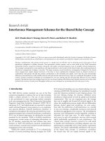
Figure 3: The per formance of the myopic policy (N = 3, L = 2,
p
(1)
11
= 0.95, p
(1)
01
= 0.05, p
(2)
11
= 0.65, and p
(2)
01
= 0.3.).
have the smallest probability of being in state 1 at each level.
From Lemma 4, the independence of the states (conditioned
on the past observations) and ordering conditions (16)on
the initial system belief vector still hold in the next slot with
channel ordering (n
2
, , n
N
, n
1
).Byinduction,itiseasyto

see that the myopic policy has a round robin structure with
circular ordering (n
1
, n
2
, , n
N
).
Theorems 1 and 2 show that the myopic policy is
a round-robin scheme (see Figure 2 where N
= 3) for
stochastically identical channels under certain conditions.
This semiuniversal structure leads to robustness against
model mismatch and variations.
5. Simulation Examples
In this section, we illustrate the performance and robustness
of the myopic policy for independent and stochastically
identical channels. Based on Theorem 1, the myopic policy
is implemented in the following steps.
Step 1. Obtain the initial channel ordering (n
1
, n
2
, , n
N
),
that is, , ω
(k)
n
1

(1) ≥ ω
(k)
n
2
(1) ≥···≥ω
(k)
n
N
(1) for all 1 ≤ k ≤ L.
Step 2. In the first slot, the myopic policy chooses channel n
1
to sense.
Step 3. For any t(t
≥ 1), if the currently sensed channel (say
n
i
) is idle, then we will sense it ag ain in slot t + 1. Otherwise
we sense the next channel (i.e., channel n
i+1
if 1 ≤ i<Nor
channel n
1
if i = N) in the circular ordering (n
1
, n
2
, , n
N
).
In Figure 3, the system belief vector starts from the

stationary distributions of the underlying Markov pro-
cesses. For this example, the conditions in Theorem 1
are satisfied and the myopic policy obeys a round robin
EURASIP Journal on Advances in Signal Processing 7
123456789
0.65
0.7
0.75
0.8
0.85
0.9
0.95
Time slot
Model variation
Normalised throughput
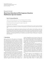
Figure 4: The robustness of the myopic policy (N = 3, L = 2. For
t
≤ 4, p
(1)
11
= 0.9, p
(1)
01
= 0.05, p
(2)
11
= 0.2, and p
(2)
01
= 0.1; for t>4,

p
(1)
11
= 0.99, p
(1)
01
= 0.69, p
(2)
11
= 0.9, and p
(2)
01
= 0.8.).
structure. We observe that the myopic policy achieves
identical performance as the optimal policy that requires
exponential complexity assumes full knowledge of the tran-
sition probabilities at all levels of the hier archical channel
model.
Figure 4 shows an example that the myopic policy
can automatically track model variations. The transition
probabilities in this example change abruptly at the fifth slot,
which corresponds to a drop in the primary t rafficload.It
can be shown that these variations will not affect the round
robin structure of the myopic policy as long as the conditions
in Theorem 1 are satisfied. From this figure, we can observe
from the change in the throughput increasing rate that the
myopic policy effectively tracks the traffic model variations
in the primary system.
We point out that when channels are independent but
stochastically nonidentical, the myopic policy is not optimal

in general. From Figure 5, we observe that the myopic
policy has a performance loss compared to the optimal one.
However, the myopic policy can stil l achieve a near optimal
performance.
Last, we show an example that the myopic policy is opti-
mal for independent and stochastically identical channels
when there are sensor errors. Under the Markovian model
(i.e., each channel h as only one level), a separ ation principle
that decouples the design of spectrum sensor and access
policies from that of the sensing policy has been established
in [14, 15]. While the separation principle may not hold
under the multiple time-scale hierarchical Markovian model,
the separate design still provides a simple and valid solu-
tion. Specifically, the spectrum sensor policy is to choose
the detection threshold such that the probability of miss
detection is equal to the maximum allowable probability of
collision to the primary users. The access policy is simply
to trust the detection outcome. Using these designs of the
spectrum sensor and the access policy, we then design the
The optimal policy
The myopic policy
0.5
0.6
0.55
0.75
0.7
12 456
Time slot
3
0.65

Normalised throughput
Figure 5: The performance of the myopic policy for nonidentical
channels (N
= 5, L = 2, p
(1)
01
= [0.20.20.40.40.4], p
(2)
01
=
[0.40.40.45 0.45 0.45], p
(1)
11
= [0. 80.80.60.60.6], and p
(2)
11
=
[0.70.70.50.50.5]).
0.6
The optimal policy
The myopic policy
Normalised throughput
Time slot
4123 5678
0.58
0.59
0.61
0.62
0.63
0.64

0.65
0.66
Figure 6: The performance of the myopic policy with sensor errors
(Prob. of false alarm
= 0.2, Prob. of miss detection = 0.3, N =
3, L = 2, p
(1)
01
= [0.05 0.05 0.05], p
(2)
01
= [0.30.30.3], p
(1)
11
=
[0.95 0.95 0.95], and p
(2)
11
= [0.65 0.65 0.65]).
sensing policy for channel selection, which is reduced to an
unconstraint POMDP problem a s addressed in this paper.
Under this design dictated by the separation principle, we
observe from Figure 6 that the myopic sensing policy can
still achieve the optimal performance for independent and
stochastically identical channels even when there are sensor
errors.
8 EURASIP Journal on Advances in Signal Processing
6. Concl usion
In this paper, we have considered the multichannel oppor-
tunistic access in self-similar primary traffic processes. Under

the assumption that the states of the Markov process are
positively correlated at each level and initially independent
across all levels for each channel, we have shown that for
independent and stochastically identical channels when the
initial system belief vector satisfies the channel ordering
condition as stated in Theorem 1, the myopic policy has a
simple and robust structure with strong performance. Future
work includes investigating the optimality and throughput
limits of the myopic policy for independent and stochasti-
cally identical channels, and extending the simple structure
of the myopic policy to nonidentical channels.
Acknowledgments
This work was supported by the Army Research Laborator y
under Grant DAAD19-01-C-0062, by the Army Research
Office under Grant W911NF-08-1-0467, and by the National
Science Foundation under Grants CNS-0627090 and CCF-
0830685. Part of this work was presented at IEEE Military
Communication Conference (MILCOM), November, 2008.
References
[1] FCC Spect rum Policy Task Force, “Report of the spectrum
efficiency,” working group, November 2002.
[2] S.Geirhofer,L.Tong,andB.M.Sadler,“Dynamicspectrum
access in the time domain: modeling and exploiting white
space,” IEEE Communications Magazine,vol.45,no.5,pp.66–
72, 2007.
[3] FCC03-322, “Notice of proposed rule making: facilitating
opportunities for flexible, efficient, and reliable spectrum use
employing cognitive radio technologies and authorization and
use of software defined radios,” December 2003.
[4] W. Leland, M. Taqqu, W. Willinger, and D. Wilson, “On the

self-similar nature of ethernet traffic,” in Proceedings of the
ACM International Conference of the Special Interest Group
on Data Communication (SIGCOMM ’93), pp. 183–193, San
Francisco, Calif, USA, September 1993.
[5] K. Park and W. Willinger, Self-Similar Network Trafficand
Performance Evaluation, John Wiley & Sons, New York, NY,
USA, 2000.
[6]M.Jiang,M.Nikolic,S.Hardy,andL.Trajkovic,“Impact
of self-similarity on wireless data network performance,”
in Proceedings of the IEEE International Communications
Conference (ICC ’01), vol. 2, pp. 477–481, June 2001.
[7] D. Radev and I. Lokshina, “Self-similar simulation of IP traffic
for wireless networks,” International Journal of Mobile Network
Design and Innovation, vol. 2, pp. 202–208, 2007.
[8] Q. Liang, “Ad hoc wireless network traffic-self-similarity and
forecasting,” IEEE Communications Letters,vol.6,no.7,pp.
297–299, 2002.
[9] V. Misra and W B. Gong, “A hierarchical model for teletraffic,”
in Proceedings of the 37th IEEE Conference on Decision and
Control (CDC ’98), vol. 2, pp. 1674–1679, Tampa, Fla, USA,
1998.
[10] W. Gong, Y. Liu, V. Misra, and D. Towsley, “Self-similarity and
long range dependence on the internet: a second look at the
evidence, origins and implications,” Computer Networks, vol.
48, no. 3, pp. 377–399, 2005.
[11] Q. Zhao, L. Tong, and A. Swami, “Decentralized cognitive
MAC for dynamic spectrum access,” in Proceedings of the 1st
IEEE International Symposium on New Frontiers in Dynamic
Spectrum Access Networks (DySPAN ’05), pp. 224–232, Balti-
more, Md, USA, November 2005.

[12] Q. Zhao, L. Tong, A. Swami, and Y. Chen, “Decentralized
cognitive MAC for opportunistic spectrum access in ad hoc
networks: a POMDP framework,” IEEE Journal on Selected
Areas in Communications, vol. 25, no. 3, pp. 589–599, 2007.
[13] Q. Zhao and A. Swami, “A decision-theoretic framework for
opportunistic spectrum access,” IEEE Wireless Communica-
tions, vol. 14, no. 4, pp. 14–20, 2007.
[14] Y. Chen, Q. Zhao, and A. Swami, “Joint design and separation
principle for opportunistic spectrum access,” in Proceedings o f
IEEE Asilomar Conference on Signals, Systems, and Computers
(ASLIOMAR ’06), pp. 696–700, Pacific Grove, Calif, USA,
October-November 2006.
[15] Y. Chen, Q. Zhao, and A. Swami, “Joint design and separation
principle for opportunistic spectrum access in the presence of
sensing errors,” IEEE Transactions on Information Theory, vol.
54, no. 5, pp. 2053–2071, 2008.
[16] Q. Zhao, B. Krishnamachari, and K. Liu, “On myopic sensing
for multi-channel opportunistic access: structure, optimality,
and performance,” IEEE Transactions on Wireless Communica-
tions, vol. 7, no. 12, pp. 5431–5440, 2008.
[17] S. H. Ahmad, M. Liu, T. Javidi, Q. Zhao, and B. Krish-
namachari, “Optimality of myopic sensing in multi-channel
opportunistic access,” to appear in IEEE Transactions on
Information Theory.
[18] O. Sheluhin, S. Smolskiy,, and A. Osin, Self-Similar Processes in
Telecommunications, John Wiley & Sons, New York, NY, USA,
2007.