Advances in Sonar Technology 2012 Part 7 doc
Bạn đang xem bản rút gọn của tài liệu. Xem và tải ngay bản đầy đủ của tài liệu tại đây (2.3 MB, 20 trang )
Independent Component Analysis for Passive Sonar Signal Processing
105
(a)
(b)
(c)
Fig. 14. DEMON analysis for both raw-data (measured acoustic signal) and frequency
domain independent components (FD-ICA) at bearings (a) 076°, (b) 190° and (c) 205°.
Advances in Sonar Technology
106
different scaling factors and ordering (Hyvärinen et al., 2001). As in the frequency-domain
BSS approach the ICA algorithms are executed after DEMON estimation at each time
window, independent components from a certain direction may appear in different ordering
at adjacent time-windows in this sequential procedure. Before generating the average
spectrum, the independent components must be reordered (to guarantee that the averages
are computed using samples from the same direction) and normalized in amplitude. The
normalization is performed by converting signal amplitude into dB scale. The reordering
procedure is executed by computing the correlation between independent components
estimated from adjacent time slots. High correlation indicates that these components are
related to the same direction.
Separation results obtained through this approach are illustrated in Fig. 14. It can be seen
that, the interfering frequencies were considerably attenuated at the independent
components from all three directions. The higher frequency noise levels were also reduced.
The results obtained from both time (ICA) and frequency domain (FD-ICA) methods are
summarized in Table 1 (when Fx frequency width is not available it means that half of Fx
peak amplitude is under the noise level). It can be observed that, for FD-ICA both the
interference peaks and the width of the frequency components belonging to each direction
were reduced, allowing better characterization of the target. The time domain method (ICA)
produced relevant separation results only for 205° signal.
Freq. Raw-data ICA FD-ICA Raw-data ICA FD-ICA
FB
-1,7 -0,8 -3,6 - - -
FC
000 87,98,4
FD
-1,4 -3,1 -1,3 - - -
FA
0 0 0 4,9 4,9 4,3
2FA
-1,4 -1,4 -1,7 5,3 5,3 4,3
3FA
-4,1 -4,1 -5,7 8,8 8,8 6,2
4FA
-5 -5 -6,7 - - 7,4
5FA
-5,3 -5,4 -7,2 - - 11
FB
-4,2 -4,1 -9,8 16,6 15,8 -
FC
-4,4 -4,4 -8,6 7,7 7,7 -
FD
-8,7 -8,6 -16,5 - - -
FA
-5,9 -9,1 -9,9 - - -
FB
0 0 0 16,8 16,3 15,2
FC
-3,2 -4,2 -6,4 7 6,6 6,5
FD
-5,6 -5,8 -9,3 - - -
Direction 190
Direction 076
Direction 205
Peak (dB) Width (RPM)
Table 1. Separation results summary
4.4 Extensions to the basic BSS model
In order to obtain better results in signal separation and thus higher interference reduction,
more realistic models may be assumed for both the propagation channel and measurement
system.
For example, it is known that, signal transmission in passive sonar problems may comprise
different propagation paths, and thus the measured signal may be a sum of delayed and
Independent Component Analysis for Passive Sonar Signal Processing
107
mixed versions of the acoustic sources. This consideration leads to the so-called convolutive
mixture model for the ICA (Hyvarinen et al., 2001), for which the observed signals x
i
(t) are
described through Eq. 10:
1
, 1
n
iikjj
jk
x
(t) a s (t k ) for i , ,n
=
=−=
∑∑
(10)
where s
j
are the source signals. To obtain the inverse model, usually a finite impulse
response (FIR) filter architecture is used to describe the measurement channel.
Another modification that may allow better performance is to consider, in signal separation
model, that sensors (or propagation channel) may present some source of nonlinear
behavior (which is the case in most passive sonar applications). The nonlinear ICA
instantaneous mixing model (Jutten & Karhunen, 2003) is thus defined by:
F( )
=
xs
(11)
where F(.) is a R
N
→ R
N
nonlinear mapping (the number of sources is assumed to be equal to
the number of observed signals) and the purpose is to estimate an inverse transformation G :
R
N
→ R
N
:
G( )
=
sx
(12)
so that the components of y are statistically independent. If G = F
−1
the sources are perfectly
recovered (Hyvärinen & Pajunen, 1999).
Some algorithms have been proposed for the nonlinear ICA problem (Jutten & Karhunen,
2003), a limitation inherit to this model is that, in general, there exists multiple solutions for
the mapping G in a given application. If x and y are independent random variables, it is
easy to prove that f(x) and g(y), where f(.) and g(.) are differentiable functions, are also
independent. A complete investigation on the uniqueness of nonlinear ICA solutions can be
found in (Hyvärinen & Pajunen, 1999). NLICA algorithms have been recently applied in
different problems such as speech processing (Rojas et al., 2003) and image denoising
(Haritopoulos et al., 2002).
Although these extensions to the basic ICA model may allow better signal separation
performance, the estimation methods usually require considerable large computational
requirements, as the number of parameters increases (Jutten & Karhunen, 2003) e
(Hyvarinen., 2001). Thus, an online implementation (which is the case in passive sonar
signal analysis) may not always be possible.
5. Summary and perspective
Sonar systems are very important for several military and civil underwater applications.
Passive sonar signals are susceptible to cross-interference from acoustic sources present at
different directions. The noise irradiated from the ship where the hydrophones are installed
may also interfere with the target signals, producing poor performance in target
identification efficiency. Independent component analysis (ICA) is a statistical signal
processing method that aims at recovering source signals from their linearly mixed versions.
In the framework of passive sonar measurements, ICA is useful to reduce signal interference
and highlight targets acoustic features.
Advances in Sonar Technology
108
Extensions to the standard ICA model, such as considering the presence of noise, multiple
propagation paths or nonlinearities may lead to a better description of the underwater
acoustic environment and thus produce higher interference reduction. Another particular
characteristic is that the underwater environment is non-stationary (Burdic, 1984).
Considering this, the ICA mixing matrix becomes a function of time. To solve the non-
stationary ICA problem recurrent neural networks trained using second-order statistic were
used in (Choi et al., 2002) and a Markov model was assumed for the sources in (Everson &
Roberts, 1999).
6. References
Brigham, E. (1988). Fast Fourier Transform and Its Applications. ISBN10: 0133075052, Ed.
FACSIMILE. 1988.
Burdic, W. S. (1984) Underwater Acoustic System Analysis, Prentice-Hall, ISBN 10- 0932146635.
Cardoso, J F. (1998). “Blind signal separation: Statistical principles”, Proceedings of IEEE, pp.
2009-2025, vol. 86 no. 10, October 1998.
Choi, S. ; Cichocki, A. and Amari, S-I (2002). Equivariant nonstationary source separation,
Neural Networks, vol. 15, no. 1, pp. 121-130, January.
Clay, C. and Medwin, H. (1998). Fundamentals of Acoustical Oceanography. ISBN:0-12-487570-
X. Academic Press.
Cover, T. M. and Thomas, J. A. (1991). Elements of Information Theory. Wiley.
Diniz, P. S. R., Silva, E., Lima Netto, S. (2002). Digital Signal Processing, ISBN: 0-521-78175-2,
Cambridge University Press.
Everson, R. and Roberts, S. J. (1999) Non-stationary Independent Component Analysis
Proceedings of the IEE conference on Artificial Neural Networks, 7 - 10 September.
Haritopoulos, H.; Yin, H. and Allinson, N. M. (2002) Image denoising using self-organizing
map-based nonlinear independent component analysis, Neural Networks, pp. 1085-
1098, 2002.
Haykin, S. (2001). Neural Networks, Principles and Practice. Bookman, ISBN: 9780132733502.
Hyvärinen, A. (1998a). New approximations of diferencial entropy for independent
component analysis and projection pursuit, Advances in Neural Information Signal
Processing, no. 10, pp. 273-279.
Hyvärinen, A. (1998b) Independent component analysis in the presence of Gaussian noise
by maximizing joint likelihood. Neurocomputing. Volume 22, Issues 1-3, November ,
Pages 49-67.
Hyvärinen, A. and Pajunen, P. (1999). Nonlinear independent component analysis: Existence
and uniqueness results, Neural Networks, vol. 12, no. 3, pp. 429-439.
Hyvärinen, A. and Oja, E. (2000). Independent component analysis: Algorithms ans applications.
Helsinki University of Technology, P. O. Box 5400, FIN-02014 HUT, Filand. Neural
Networks, 13 (4-5): 411-430. 2000.
Hyvärinen, A., Karhunen, J. and Oja, E. (2001). Independent Component Analysis, ISBN: 0-471-
40540-X, John Wiley & Sons, .inc. 2001.
Jeffsers, R., Breed and B. Gallemore (2000). Passive range estimation and rate detection,
Proceedings of Sensor Array and Multichannel Signal Processing Workshop, pp. 112-116,
ISBN: 0-7803-6339-6, Cambridge, US, March 2000.
Independent Component Analysis for Passive Sonar Signal Processing
109
Jutten, C. and Karhunen, J. (2003) Advances in nonlinear blind source separation,
Proceedings of the 4th Int. Symp. on Independent Component Analysis and Blind Signal
Separation (ICA2003), Nara, Japan, pp. 245-256.
Kim, T H. and White, H. (2004) “On more robust estimation of skewness and kurtosis,”
Finance Research Letters, vol. 1, pp. 56-73.
Knight, W. C. Pridham, R. G. Kay, S. M. (1981). Digital signal processing for sonar.
Proceedings of IEEE, ISSN: 0018-9219 vol. 69, issue 11, pp. 1451-1506, November.
1981.
Krim, H. and Viberg, M. (1996) Two decades of array signal processing research: the
parametric approach. IEEE Signal Processing Magazine, vol. 13, Issue: 4, pp. 67-94,
ISSN: 1053-5888.
Lee, B. J. Park, J.B. Joo, Y. H. Jin, S. H. (2004). Intelligent Kalman filter for tracking a
manoeuvring target. Radar, Sonar and Navigation, IEE Proceedings, ISSN: 1350-2395,
vol. 151 issue: 6, pp. 344-350 Dec. 2004.
Marple, L., Brotherton, T. (1991). Detection and classification of short duration underwater
acoustic signals by Prony’s method, International Conference on Acoustics, Speech, and
Signal Processing, pp. 1309-1312 vol.2, ISBN: 0-7803-0003-3, Toronto, Ont., Canada,
May 1991.
Mellema, G. R. (2006). Reverse-Time Tracking to Enhance Passive Sonar, International
Conference on Information Fusion, ISBN: 0-9721844-6-5, pp. 1-8, July.
Moura, N. N.; Soares Filho, W.; Seixas, J. M. de (2007a). Passive Sonar Classification based
on Independent components. Proceedings of the Brazilian congress of neural networks,
2007, Florianópolis, Brazil, pp. 1-5. (In Portuguese).
Moura, N. N., Seixas, J. M. Soares Filho, W. and Greco, A. V. (2007b) “Independent
component analysis for optimal passive sonar signal detection,” Proceedings of the
7th International Conference on Intelligent Systems Design and Applications, Rio de
Janeiro, pp. 671-678, October 2007.
Nielsen, R. O. (1991). Sonar Signal Processing, ISBN: 0-89006-453-9. Artech House Inc,
Nortwood, MA, 1991.
Nielsen, R. O. (1999). “Cramer-Rao lower bounds for sonar broadband modulation
parameters”. IEEE Journal of Ocean Engineering, vol. 24 no. 3, pp. 285-290, July 1999.
Papoulis,A. (1991), Probability, Random Variables, and Stochastic Processes. McGraw-Hill.
Peyvandi, H., Fazaeefar, B., Amindavar, H (1998). Determining class of underwater vehicles
in passive sonar using hidden Markov with Hausdorff similarity measure,
Proceedings of 1998 International Symposium on Underwater Technology, pp. 258-
261,ISBN: 0-7803-4273-9, Tokyo, Japan, April 1998.
Rao, S. K. (2006). Pseudo linear Kalman filter for underwater target location using intercept
sonar measurements. Symposium of Position, location and navigation, ISBN: 0-7803-
9454-2. Pp. 1036-1039, San Diego, US, April 2006.
Rojas, F.; Puntonet, C. G. and Rojas, I. (2003) Independent component analysis evolution
based method for nonlinear speech processing, Artificial Neural Nets Problem Solving
Methods, PT II, vol. 2687, pp. 679-686, 2003.
Seixas, J. M., Mamazio, D. O., Diniz, P. S. R., Soares-Filho, W. (2001). Wavelet transform as a
preprocessing method for neural classification of passive sonar signals, The 8
th
IEEE
International Conference on Electronic, Circuits and Systems, pp. 83-86, ISBN: 0-7803-
7057-0, Malta, September 2001.
Advances in Sonar Technology
110
Shannon, C. E. (1948). “A mathematical theory of communication,” The Bell System Technical
Journal, pp. 379-423, July.
Shaolin Li, Sejnowski, T. J. (1995). Adaptive separation of mixed broadband sound sources
with delays by a beamforming Herault-Jutten network. IEEE Journal of Oceanic
Engineering, ISSN: 0364-9059, vol. 20, pp. 73-79, 1995.
Soares Filho, W.; Seixas, J. M. de; Calôba, L. P. (2001) Principal Component Analysis for
Classifyting Passive Sonar Signals. IEEE International Symposium on Circuits and
Systems, 2001, Sidney, Australia.
Spiegel, M. R., Schiller, J. J. and Srinivasan, R. A. (2000). Probability and Statistics. McGraw-
Hill, 2 ed.
Torres, R. C.; Seixas, J. M. de, Soares Filho, W. (2004) Sonar Signals Classification Through
Non-linear Principal Component Analysis. Learning and nonlinear models. Vol. I, no.
4, pp. 208-222, 2004 (In Portuguese).
Trees, H. L. V. (2001) Detection, Estimation and Modulation Theory – Part I, ISBN: 0-471-09517-
6, John Wiley & Sons, Inc.
Waite, A. D. (2003). Sonar for practicing Engineers, ISBN: 0-471-49750-9, John Wiley and Sons,
New York, 2003
Welling, M. (2005) Robust higher order statistics, Proceedings of the Tenth International
Workshop on Artificial Intelligence and Statistics (AISTATS2005), pp. 405-
412,Barbados, January.
Yan, D. P. and Peach, J. (2000). Comparison of blind source separation algorithms. Advanxes
in Neural networks and applications. Pp. 18-21. 2000.
Yang, Z., Yang, L., Qing, C., Huang, D (2007) An improved empirical
AM/FMdemodulation method. International Conference on Wavelet Analysis and
Pattern Recognition. ISBN: 978-1-4244-1065-1, vol. 3, pp. 1049-1053.
6
From Statistical Detection to Decision Fusion:
Detection of Underwater Mines
in High Resolution SAS Images
Frédéric Maussang
1
, Jocelyn Chanussot
2
, Michèle Rombaut
2
and Maud Amate
3
1
Institut TELECOM; TELECOM Bretagne; UeB; CNRS UMR 3192 Lab-STICC
2
GIPSA-Lab (CNRS UMR 5216); Grenoble INP
3
Groupe d’Etudes Sous-Marines de l’Atlantique DGA/DET/GESMA Brest
France
1. Introduction
Among all the applications proposed by sonar systems is underwater demining. Indeed,
even if the problem is less exposed than the terrestrial equivalent, the presence of
underwater mines in waters near the coast and particularly the harbours provoke accidents
and victims in fishing and trade activities, even a long time after conflicts.
As for terrestrial demining (Milisavljević et al., 2008), detection and classification of various
types of underwater mines is currently a crucial strategic task (U.S. Department of the Navy,
2000). Over the past decade, synthetic aperture sonar (SAS) has been increasingly used in
seabed imaging, providing high-resolution images (Hayes & Gough, 1999). However, as with
any active coherent imaging system, the speckle constructs images with a strong granular
aspect that can seriously handicap the interpretation of the data (Abbot & Thurstone, 1979).
Many approaches have been proposed in underwater mine detection and classification
using sonar images. Most of them use the characteristics of the shadows cast by the objects
on the seabed (Mignotte et al., 1997). These methods fail in case of buried objects, since no
shadow is cast. That is why this last case has been less studied. In such cases, the echoes
(high-intensity reflection of the wave on the objects) are the only hint suggesting the
presence of the objects. Their small size, even in SAS imaging, and the similarity of their
amplitude with the background make the detection more complex.
Starting from a synthetic aperture image, a complete detection and classification process
would be composed of three main parts as follows:
1. Pixel level: the decision consists in deciding whether a pixel belongs to an object or to the
background.
2. Object level: the decision concerns the segmented object which is “real” or not: are these
objects interesting (mines) or simple rocks, wastes? Shape parameters (size,…) and
position information can be used to answer this question.
3. Classification of object: the decision concerns the type of object and its identification (type
of mine).
This chapter deals with the first step of this process. The goal is to evaluate a confidence that
a pixel belongs to a sought object or to the seabed. In the following, considering the object
Advances in Sonar Technology
112
characteristics (size, reflectivity), we will always assume that the detected objects are actual
mines. However, only the second step of the process previously described, which is not
addressed in the chapter, would give the final answer.
We propose in the chapter a detection method structured as a data fusion system. This type
of architecture is a smart and adaptive structure: the addition or removal of parameters is
easily taken into account, without any modification of the global structure. The inputs of the
proposed system are the parameters extracted from an SAS image (statistical in our case).
The outputs of the system are the areas detected as potentially including an object.
The first part of the chapter presents the main principal of the SAS imaging and its use for
detection and classification. The second part is on the extraction of a first set of parameters
from the images based on the two first order statistical properties and the use of a mean –
standard deviation representation, which allow to segment the image (Maussang et al., IEEE,
2007). A third part enlarges this study to the higher order statistics (Maussang et al.,
EURASIP, 2007) and their interest in detection. Finally, the last part proposes a fusion
process of the previous parameters allowing to separate the regions potentially containing
mines (“object”) from the others (“non object”). This process uses the belief theory (Maussang
et al., 2008). In order to assess the performances of the proposed classification system, the
results, obtained on real SAS data, are evaluated visually and compared to a manually
labeled ground truth using a standard methodology (Receiver Operating Characteristic
(ROC) curves).
2. SAS technology and underwater mines detection
SAS (Synthetic Aperture Sonar) history is closely linked to the radar one. Actually, the
airborne radar imagery was the first to develop the process of synthetic aperture in the
1950’s (SAR : Synthetic Aperture Radar). Then, it was applied to satellite imagery. The first
satellite to use synthetic aperture radar was launched in 1978. Civilian and military
applications using this technique covered enlarged areas with an improved resolution cell.
Such a success made the synthetic aperture technique essential to obtain high resolution
images of the earth. Following this innovation, this technique is now frequently used in
sonar imagery (Gough & Hayes, 2004). The first studies in synthetic aperture sonar occurred
in the 1970’s with some patents (Gilmour, 1978, Walsh, 1969, Spiess & Anderson, 1983) and
articles on SAS theory by Cutrona (Cutrona, 1975, 1977).
2.1 SAS principle
Synthetic aperture principle is presented on Fig. 1 and consists in the coherent integration of
real aperture beam signals from successive pings along the trajectory. Thus, the synthetic
aperture is longer than the real aperture. As the resolution cell is inversely proportional to
the length of the aperture, longer the antenna, better the resolution. In practice, the synthetic
aperture depends on the movements of the vehicle carrying the antenna. Movements like
sway, roll, pitch or yaw are making the integration along the trajectory more difficult.
The synthetic aperture resolution is that of the equivalent real aperture of length L
ERA
, given
by the expression:
RERA
)1(2 LVTNL
+
−
=
(2.1)
From Statistical Detection to Decision Fusion: Detection of Underwater Mines
in High Resolution SAS Images
113
Fig. 1. SAS principle
where N is the number of pings integrated, V is the mean cross-range speed, T is the ping
rate and L
R
is the real aperture length.
Hence, the cross-range resolution at range R is given by:
ERA
S
L
R
λ
δ
=
(2.2)
The maximum travel length (N-1)VT corresponds normally (but not necessarily) to the
cross-range width of the insonification sector, equal to Rλ/L
tr
when the transmitter has a
uniform phase-linear aperture of length L
tr
and operates in far field. For large N, the L
ERA
given by (2.1) equals approximately twice this width; hence, the resolution is independent
of range and frequency, and is given by the expression:
2
tr
S
L
=
δ
(2.3)
Let us note that the cross-range resolution of the physical array δ
R
= Rλ/L
R
. The resolution
gain g of the synthetic aperture processing is defined by the expression:
R
ERA
S
R
L
L
g ==
δ
δ
(2.4)
2.2 SAS challenges
Nowadays, SAS is a mature technology used in operational systems (MAST’08). However,
some challenges remain to enhance SAS performances. For example, a precise knowledge of
the motion of the antenna will permit to obtain a better motion compensation and better
focused images. There are also some studies to improve beamforming algorithms, more
adapted to SAS processing. Another challenge lies in the reduction of the sonar frequency.
Knowing that sound absorption increases with the frequency in environments like sea water
or sediment, a logical idea is to decrease imagery sonar frequency. Yet, resolution is
inversely proportional to frequency and length of antenna. So for a reasonable size of array,
Advances in Sonar Technology
114
the resolution remains quite low, especially for underwater minewarfare. SAS processing
can then be used to artificially increase the length of the antenna and improve the resolution
One of the purposes is the detection of objects buried in the sediment. Both civilian (pipeline
detection, wreck inspection) and military (buried mines detection) applications are
interested in this concept. GESMA conducted numerous sea experiments on SAS subject
since the end of the 1990’s. Firstly, in 1999, in cooperation with the British agency DERA,
high frequency SAS was mounted on a rail in Brest area (Hétet, 2000). The central frequency
was 150 kHz, the frequency band was 60 kHz and the resolution obtained was 4 cm. Fig. 2
presents two images resulting from this experiment.
Fig. 2. On the left, SAS image and picture of the associated modern mine. On the right, SAS
image and picture of the associated modern mines
Then, GESMA decided to work on buried mines and conducted an experiment with a low
frequency SAS mounted on a rail in 1999. It was in Brest area, the sonar frequency was
between 14 and 20 kHz (Hétet, 2003). Fig. 3 presents results of this experiment. We notice
the presence of a large echo coming from the cylinder.
Fig. 3. SAS image of buried and proud objects at 20 m. C1 : buried cylinder ; R1 : buried
rock ; S1 : buried sphere ; S2 : proud sphere
Fig. 3 shows that low frequencies allow to penetrate the sediment and to detect buried
objects. Moreover, echoes are more contrasted on this image and there is a lack of the
From Statistical Detection to Decision Fusion: Detection of Underwater Mines
in High Resolution SAS Images
115
shadows for the objects, making the classification more difficult. To go a step further, in
2002, a low frequency SAS was hull mounted onboard a minehunter (Hétet et al., 2004).
Frequency was chosen between 15 and 25 kHz and Fig. 4 presents results of these trials
conducted in cooperation with the Dutch agency TNO, Defence, Security and Safety.
Fig. 4. Low frequency SAS images. On the left, SAS image of three cylinders.
Downwards : proud cylinder, half buried cylinder, buried cylinder. In the middle : pictures
of the supporting ship, the sonar and the three cylinders. On the right, SAS images of two
wrecks in the bay of Brest.
Considering previous figures, low frequency and high frequency SAS images present an
important difference. High frequency images allow detecting and classifying underwater
objects thanks to their shadow when low frequency images present no more shadow but
strong echoes. The idea is thus to use specificities of low frequency SAS to define a new
approach to detect and classify buried objects.
3. Underwater mines detection using local statistical parameters
The key issue when designing a classification algorithm is to choose the right parameters
discriminating the classes of interest. The two main approaches are (i) use of statistical
knowledge about the process, (ii) use of expert knowledge, eventually derived from a
physical model of the process. In this application, the statistical characteristics of the seabed
pixels are well known and follow statistical laws (Rayleigh and Weibull distributions for
instance). As a consequence, the data fusion process is based on the comparison of the
statistical characteristics locally extracted for each pixel and these laws.
3.1 Statistical description of the SAS images
The sonar images, as any image formed by a coherent system (radar imagery is another
example), are seriously corrupted by the speckle effect. They thus have a strong granular
aspect. This noise comes from the presence of a large number of elements (sand, rocks, etc.)
that are smaller than the wavelength and randomly distributed over the seabed. The sensor
receives the result of the interference of all the waves reflected by these small scatterers
within a resolution cell (Goodmann, 1976).
Advances in Sonar Technology
116
3.1.1 Speckle noise and the Rayleigh law
Sonar images provided by the sonar system are constructed by the speckle. This bottom
reverberation comes from the presence of a large number of elements (sand, gravel, etc.) that
are smaller than the wavelength of the used monochromatic and coherent illumination
source. These elements are assumed to be randomly distributed on the seabed. As a
consequence, the sensor records the result of the constructive and destructive interferences
of all the waves reflected by these elementary scatterers contained in a resolution cell (Collet
et al., 1998, Schmitt et al., 1996).
The response of a resolution cell can thus be described by the following:
∑
=
+===
d
N
i
ii
YjXjAja
1
.)exp()exp(
φϕρ
(3.1)
with A being the amplitude of the response on a resolution cell and
φ
representing the
phase. The phases are usually considered as independent and uniformly distributed
over
],[
π
π
+−
. With these assumptions, and if the number of elementary scatterers N
d
within the resolution cell is large enough, the central limit theorem applies: X and Y can be
considered as Gaussian random values. Consequently, the probability density function of
amplitude
22
YXA += follows a Rayleigh distribution:
0,
2
exp)(
2
2
2
≥
⎟
⎟
⎠
⎞
⎜
⎜
⎝
⎛
−= A
AA
Ap
A
R
αα
(3.2)
with α being the Rayleigh’s law specific parameter. This parameter is bound with the
average intensity of the reflected waves.
The νth-order moment of A is given by the following:
⎟
⎠
⎞
⎜
⎝
⎛
+Γ=
2
1)2(
2/2
)(
ν
αμ
ν
ν
A
(3.3)
with Γ being the Gamma function (
∫
+∞
−
==+Γ
0
!)1( dttezz
zt
). This results in an interesting
property of the Rayleigh law: the standard deviation σ
A
and the mean μ
A
of the amplitude A
are linked by a simple proportionality relation:
ARA
k
σ
μ
=
=
with 91.1
4
≈
−
=
π
π
R
k (3.4)
This property leads to modeling the speckle as a multiplicative noise. As a matter of fact, the
variation of amplitude induced by the speckle and characterized by parameter σ
A
is bound
by the mean amplitude (μ
A
) with a multiplicative coefficient k
R
.
3.1.2 Non-Rayleigh models
The previous description of the speckle is the most usual and the most popular one.
However, it is not satisfactory when the number of scatterers within a resolution cell (noted
From Statistical Detection to Decision Fusion: Detection of Underwater Mines
in High Resolution SAS Images
117
N
d
in the previous paragraph) significantly decreases. The central limit theorem does not
hold and the Rayleigh approximation is no longer valid. This case is frequently observed in
high-resolution images (Collet et al., 1998, Mignotte et al., 1999) such as SAS images. In this
case, the amplitude A is better described by a Weibull law:
0,exp)(
1
≥
⎥
⎥
⎦
⎤
⎢
⎢
⎣
⎡
⎟
⎟
⎠
⎞
⎜
⎜
⎝
⎛
−
⎟
⎟
⎠
⎞
⎜
⎜
⎝
⎛
=
−
A
AA
Ap
A
W
δδ
βββ
δ
(3.5)
with β being the scale parameter and δ representing the shape parameter, strictly positive.
These two parameters provide an increased flexibility compared to the Rayleigh law. Note
that this law is a simple generalization of the Rayleigh distribution (in the special case
αβ
2= and δ = 2, the Weibull law turns to a simple Rayleigh law).
For a Weibull distribution, the νth-order moment of A is given by:
⎟
⎠
⎞
⎜
⎝
⎛
+Γ=
δ
ν
βμ
ν
ν
1
)(A
(3.6)
Therefore, the proportionality between and still holds, but with a coefficient k
W
(δ ) function
of δ:
2
)/11()/21(
)/11(
)(
δδ
δ
δ
+Γ−+Γ
+
Γ
=
W
k (3.7)
Note that for δ = 2, corresponding to the Rayleigh law, we obtain the same coefficient as in
(3.4).
Other more complex non-Rayleigh approaches have been proposed in the literature to
statistically describe the bottom reverberation in high-resolution sonar imaging. One of the
most famous models is the K-distribution. For this model, the number of scatterers in a
resolution cell N
d
is supposed to be a random variable following a negative binomial
distribution. The amplitude A is then described by a K-law (called generalized K-
distribution), a three parameters distribution function given by (Gu & Abraham, 2001):
0,2
)()(
4
)(
10
1
1010
10
01
10
≥
⎟
⎟
⎠
⎞
⎜
⎜
⎝
⎛
⎟
⎟
⎠
⎞
⎜
⎜
⎝
⎛
ΓΓ
=
−
−+
AAKAAp
A
K
μ
νν
μ
νν
μ
νν
νν
νν
νν
(3.8)
where ν
1
is the shape parameter, µ is the scale parameter, and ν
0
is the parameter bound to
the number of raw data averaged to figure out the pixel reflectivity. K
ν1- ν0
is the modified
Bessel function of the second kind and order ν
1
- ν
0
. This distribution describes a rapidly
fluctuating Rayleigh component modulated by a slowly varying χ² component.
The νth-order moment of A is then given by:
)()(
)2/()2/(
10
10
2
10
)(
νν
νννν
νν
μ
μ
ν
ν
ΓΓ
+Γ+Γ
⎟
⎟
⎠
⎞
⎜
⎜
⎝
⎛
=
A
(3.9)
Advances in Sonar Technology
118
The relationship between σ
A
and μ
A
is preserved, with a coefficient depending on the two
parameters ν
1
and ν
0
:
2
1
2
0
2
1
2
010
10
10
)2/1()2/1()()(
)2/1()2/1(
),(
+Γ+Γ−ΓΓ
+Γ+Γ
=
νννννν
νν
νν
K
k (3.10)
A Rayleigh mixture has been also proposed to describe SAS data, each scattering material
within a resolution cell being characterized by one specific Rayleigh distribution (Hanssen et
al., 2003).
3.1.3 Application to experimental data
In this section, the performances of the different statistical models are compared using the
SAS data presented in section 2 (Fig. 2). For this purpose, two tests are considered: the χ²
criterion and the Kolmogorov distance (Mignotte et al., 1999). The χ² criterion d
χ²
is estimated
according to the following relation (Saporta, 1990):
(
)
∑
=
−
=
r
i
i
ii
nP
nPk
d
1
2
2
χ
(3.11)
where k
i
is the number of realizations (number of pixels having the value i), P
i
is the
estimated probability of value i, r is the number of possible values, and n is the number of
observations (in our case, the number of pixels).
With k’
i
being the number of realizations from 1 to i and p’
i
being the value for i of the
cumulative distribution function associated with p
i
, the Kolmogorov distance is defined as:
ii
ri
K
pnkd
′
−
′
=
= 1
max (3.12)
The parameters of the Rayleigh and the Weibull laws are evaluated on the SAS image using
a maximum-likelihood (ML) estimator. The estimated parameter
ML
α
ˆ
of the Rayleigh law
(3.2) is given by the following (Schmitt et al., 1996):
∑
=
=
n
i
iML
y
n
1
22
2
1
ˆ
α
(3.13)
where n is the number of pixels and y
i
is the amplitude of pixel i.
Parameters β and δ of the Weibull law (3.5) are estimated by
ML
β
ˆ
and
ML
δ
ˆ
, respectively,
given by the following (Mignotte et al., 1999):
k
k
ML
δδ
+∞→
= lim
ˆ
(3.14)
ML
ML
n
i
iML
y
n
δ
δ
β
ˆ
/1
1
ˆ
1
ˆ
⎟
⎟
⎠
⎞
⎜
⎜
⎝
⎛
=
∑
=
(3.15)
From Statistical Detection to Decision Fusion: Detection of Underwater Mines
in High Resolution SAS Images
119
with δ
k
= F(δ
k-1
), δ
0
= 1 (exponential law), and
()
∑∑∑
∑
===
=
−
=
n
i
x
i
n
i
i
n
i
i
x
i
n
i
x
i
yyyyn
yn
xF
111
1
lnln
)(
(3.16)
These estimators are unbiased, consistent, and efficient (Collet et al., 1998).
The estimation of the K-law parameters is more problematic. Actually, there is no analytic
expression for the derivative of a modified second kind Bessel function. Consequently, no
ML estimation can be performed without approximations (Joughin et al., 1993). A moment’s
method can then be used (3.9), even though it does not offer a closed-form solution.
These estimators are tested on the image presented in section 2 (Fig. 2 left). Fig. 5 presents in
solid line the observed distribution (normalized histogram of the image) and compares it
with the estimated Rayleigh and Weibull distributions (dashed lines).With a simple visual
inspection, one immediately notices that the Weibull distribution and K-distribution fit the
observed one better than the Rayleigh distribution
1
. This confirms the nonvalidity of the
central limit theorem in the case of high-resolution images obtained in SAS imaging. This
Rayleigh model will not be used subsequently. It is nevertheless included in this chapter
Fig. 5. Rayleigh distribution, Weibull distribution, and K-distribution estimated on Fig. 2
1
In Fig. 2 a shadow can be seen behind the echoes reflected by the mine. Shadows are
present on most sonar images containing underwater mines lying on the seabed. The
shadow corresponds to a non illuminated region of the seabed and the sensor receives a
weak acoustic wave from this region: the signal related to the shadow area essentially
consists of the electronic noise from the processing chain. It can also come from the
“differential shadow effect” due to the variation of the shadow zone position during the
imaging process. The amplitude A of the pixels in this region can thus also be modeled by a
Gaussian distribution and the models remain valid.
Advances in Sonar Technology
120
since the reader dealing with low-resolution sonar images may use the very same detection
method proposed in this paper using the Rayleigh distribution. The K-distribution seems to
provide a better statistical model of the background than the Weibull law. It especially fits
better the “head” of the observed distribution. This is confirmed by the quantitative
evaluation presented in Table 1. However, the “tail” of the distribution is accurately
estimated by both models.
Distribution
Estimated
parameters
χ
2
criterion
Kolmogorov
distance
Rayleigh
5.1482
ˆ
≈
ML
α
357.9 2.22 x 10
-4
Weibull
7.1961
ˆ
≈
ML
β
604.1
ˆ
≈
ML
δ
0.318 1.66 x 10
-4
K
6
10300.4
ˆ
×≈
μ
882.0
ˆ
0
≈
ν
163.3
ˆ
1
≈
ν
0.044 1.41 x 10
-4
Table 1. Comparison of the performances of the distribution on the SAS image of Fig. 2
3.1.4 Choice of the statistical model
Considering the previous remarks, the K-distribution seems to be a better model than the
Weibull model. However, as we have seen in section 3.1.2, the estimation of K-law
parameters is more difficult (no ML estimators). The estimators of the K-parameters are not
optimal and the estimation takes more time.
The difference with the Weibull model is not enough to justify this difficulty. Moreover,
Weibull law is largely used in the sonar community and it made its proofs in their
applications. That is why we will use the Weibull model in the following, but we keep in
mind the existence of other models such as K.
3.1.5 Local statistical description
In the previous sections, a global statistical description of the SAS images has been given,
ignoring the presence of any echoes. This is fair since the number of target pixels in the image
is too small to significantly modify the global statistics. The observed histogram matches
indeed very well a Weibull law. In this section, we study local first- and second-order
statistical properties. This is achieved by looking at the data through a small sliding window
composed of few pixels. In this case, the potential presence of echoes can no longer be ignored.
Each echo is modeled as a deterministic element with an amplitude D surrounded by a
noisy background with a Weibull distribution. We assume that the noise correlation is
smaller than the spatial extension of the target echo and that the amplitude fluctuation of
the echo is negligible. This is consistent with the experiments where the echoes appear as
small sets of connected pixels with an almost constant value. This is justified in Fig. 8(b)
with the pixels corresponding to echoes fitting the predicted ellipse in the mean–standard
deviation plane.
We note p the proportion of deterministic pixels (i.e., pixels belonging to an echo) and (1 – p)
the proportion of random values (i.e., pixels belonging to the background) within a small
square window (Fig. 6). Considering μ’
D(r)
, μ’
N(r)
, and μ’
W(r)
, the rth-order noncentral
From Statistical Detection to Decision Fusion: Detection of Underwater Mines
in High Resolution SAS Images
121
moments computed on the “echo part” of the window, the “background part” of the
window, and the whole window, respectively, the following relation holds:
)()()(
)1(
rNrDrW
pp
μμμ
′
−+
′
=
′
(3.17)
Considering μ
X
= μ’
X(1)
and σ²
X
= μ’
X(2)
- μ’²
X(1)
, the mean and the variance of X, respectively
[X can be replaced by D, N, or W, as in (3.17)], we have:
NW
pDp
μ
μ
μ
)1(
−
+
=
(3.18)
(
)
(
)
(
)
222222
1
WNNDDW
pp
μμσμσσ
−+−++= (3.19)
Moreover, echoes are considered as deterministic elements with an amplitude D, leading to:
r
rD
D=
′
)(
μ
(3.20)
and
D
D
=
μ
and 0
=
D
σ
(3.21)
and, consequently:
(
)
NNW
Dp
μ
μ
μ
−
+
=
(3.22)
(
)
2222222
NNWNNW
Dp
μσμμσσ
−−+−+= (3.23)
By combining (3.22) and (3.23), we obtain an interesting relationship between σ
W
and μ
W
:
(
)
(
)
DD
NWNWW
NN
μλμλμμσ
σσ
−+−+=+
22
(3.24)
with
(
)
NN
D
N
μσλ
σ
−= /
2
. It is important to underline that this relation is independent of p.
Also note that in limit cases, this relation remains valid: in the case of p = 0 (the window
contains only background pixels), μ
W
= μ
N
and σ
W
= σ
N
; in the case of p = 1 (the echo is
filling the whole window), μ
W
= D and σ
W
= 0, which is consistent with (3.21). Remember
that intermediate values of p correspond to windows being partially composed of echo
pixels.
3.2 First and second order parameters: segmentation
The proportional relation of the statistical model describing the sea bed sonar data previously
described is used to extract the two first parameters. The local mean and standard deviation
are estimated on the SAS image using a square sliding window. These values become the
coordinates of the processed pixel in the mean – standard deviation plane.
3.2.1 Mean-standard deviation representation
Inspired by a segmentation tool applied to spectrograms (Hory et al., 2002), this enables the
separation of the echoes from the bottom reverberation, both features having different
statistical characteristics as stated in section 3.1. In (Ginolhac et al., 2005), the link between
first- and second-order statistics is highlighted using this representation.
Advances in Sonar Technology
122
Fig. 6. Modeled echo and various values of the parameter p: (a) p = 0, (b) p = 1/9, (c) p = 2/9,
and (d) p = 1
Fig. 7. Building of the mean–standard deviation representation
Whereas in (Ginolhac et al., 2005) this link is simply illustrated as a justification to use first-
and second-order statistics, the method presented in this chapter actually performs a
segmentation of the mean–standard deviation plane.
The idea is to change the representation space of the data to highlight local statistical
properties. The chosen space is the mean–standard deviation plane. For each pixel, the local
standard deviation and the local mean are estimated within a square-centered computation
window with the following conventional equations:
∑
=
=
N
i
iW
y
N
1
1
ˆ
μ
(3.25)
()
∑
=
−=
N
i
WiW
y
N
1
2
ˆ
1
ˆ
μσ
(3.26)
From Statistical Detection to Decision Fusion: Detection of Underwater Mines
in High Resolution SAS Images
123
where N is the number of pixels in the computation window ( N = N
x
.N
y
with N
x
and N
y
being the length and the width of the window, respectively) and y
i
is the value of pixel in
the window. The pair
(
)
WW
μ
σ
ˆ
,
ˆ
becomes the coordinates representing the current pixel in
the mean–standard deviation plane (Fig. 7). The performances of these estimators are
evaluated by computing their moments (Hory et al., 2002). For the mean estimator, the mean
()
W
M
μ
ˆ
and the variance
(
)
W
V
μ
ˆ
are:
(
)
WW
M
μ
μ
=
ˆ
(3.27)
()
N
V
W
W
2
ˆ
σ
μ
=
(3.28)
The mean estimator is unbiased and consistent with a variance varying as 1/N. For the
standard deviation estimator, the mean
(
)
W
M
σ
ˆ
and the variance
(
)
W
V
σ
ˆ
are given by:
()
(
)
()
W
WW
W
mNNN
N
M
σ
σ
σ
)4(
42
1334
2
1
ˆ
−−−−
≈
(3.29)
()
(
)
(
)
2
4
)4(
2
31
4
1
ˆ
W
WW
W
NmN
N
V
σ
σ
σ
−−−
= (3.30)
with m
W(4)
being the fourth central moment computed on the window. These equations come
from the approximation
(
)
(
)
(
)
XMXVXV 4≈ with X being a random variable (Kendall &
Stuart, 1963). This estimator is asymptotically unbiased and is consistent with a variance
varying as 1/N.
The choice of the size of the computation window is a tradeoff. On one hand, the variance of
the estimators [see (3.25) and (3.26)] increases for small values of N. N should thus not be too
small to enable an accurate estimation. On the other hand, if N is too high, echoes being
small elements, the proportion p of the deterministic elements in the computation windows
remains low and echoes are lost in the background speckle [see (3.24)]. Consequently, the
computation window should be chosen as slightly larger than the spatial extension of the
echoes, this size depending on the resolution of the sonar image and the quality of the
preprocessing chain.
The mean–standard deviation representation of Fig. 2 image is built with a 5 x 5-cm²
window and is presented in Fig. 9. A general linear orientation is observed, as well as some
pixels distancing the main direction on the right [see Fig. 8(b)]. Three different linear
regressions of the data in the mean–standard deviation plane can be computed. They are
shown in Fig. 8(a). The first line, with a slope of approximately 1.91, corresponds to the
proportionality relation between the mean and the standard deviation estimated when
assuming that the bottom reverberation is modeled by a Rayleigh law (3.4). The second line,
with a slope of approximately 1.57, corresponds to the proportionality relation estimated
with a Weibull model (3.7). At the given computation accuracy, the same line is obtained by
a linear regression using a mean square method on the pixels representatives. To describe
the global linear orientation of the data in the mean–standard deviation plane, the
Advances in Sonar Technology
124
proportionality coefficient estimated with the Weibull assumption clearly outperforms the
estimation based on a Rayleigh law. This confirms the previous results for the case of high-
resolution data (Table I). In Fig. 8(b), the curve corresponding to the local relationship
between mean–standard deviation on a computation window (3.24) is plotted considering a
deterministic element with an amplitude of D = 3.4 × 10
-4
, approximately corresponding to
the typical amplitude of the main echo on the original SAS image. This curve is a part of an
ellipse and is a fairly good estimation of the main structure. Results obtained on other data
sets could not be presented in this paper for confidentiality reasons. We will see following
that each structure can be associated with one echo on the SAS image.
(a) (b)
Fig. 8. Mean–standard deviation representation of the SAS image (5 cm x 5-cm window).
The linear approximations are estimated by the Rayleigh law, the Weibull law, and a
regression. (a) Linear approximations. (b) Echo model
(a) (b)
Fig. 9. Comparison between the SAS image (Fig. 2) and its mean–standard deviation
representation. (a) Zoom of the SAS image. (b) Representation
The fact that no pixel is on the Y-axis of this representation comes from the size of the
computation window sensibly larger than the echoes. Therefore, no window contains only