Frontiers in Adaptive Control Part 5 potx
Bạn đang xem bản rút gọn của tài liệu. Xem và tải ngay bản đầy đủ của tài liệu tại đây (510.67 KB, 25 trang )
An Adaptive Controller Design for Flexible-joint Electrically-driven Robots
With Consideration of Time-Varying Uncertainties
91
7. Appendix
Lemma A.1:
Let
n
ℜ∈s ,
n
ℜ∈ε and
K
is the nn × positive definite matrix. Then,
]
)(
)([
2
1
min
2
2
min
K
ε
sKεsKss
λ
λ
−≤+−
TT
. (A.1)
Proof:
]
)(
)([
2
1
]
)(
)([
2
1
]
)(
)([
2
1
])([
min
2
2
min
min
2
2
min
2
min
min
min
K
ε
sK
K
ε
sK
K
ε
sK
sεsKεsKss
λ
λ
λ
λ
λ
λ
λ
−−≤
−−
−−=
+−≤+−
TT
Q.E.D.
Lemma A.2:
Let
n
inii
T
i
www
×
ℜ∈=
1
21
][ Lw , i=1,…,m and W is a block diagonal matrix
defined as
mmn
m
diag
×
ℜ∈= },,,{
21
wwwW L . Then,
∑
=
=
m
i
i
T
Tr
1
2
)( wWW . (A.2)
The notation Tr(.) denotes the trace operation.
Proof: The proof is straightforward as below:
Frontiers in Adaptive Control
92
⎥
⎥
⎥
⎥
⎥
⎦
⎤
⎢
⎢
⎢
⎢
⎢
⎣
⎡
=
⎥
⎥
⎥
⎥
⎦
⎤
⎢
⎢
⎢
⎢
⎣
⎡
=
⎥
⎥
⎥
⎥
⎦
⎤
⎢
⎢
⎢
⎢
⎣
⎡
⎥
⎥
⎥
⎥
⎦
⎤
⎢
⎢
⎢
⎢
⎣
⎡
=
⎥
⎥
⎥
⎥
⎥
⎥
⎥
⎥
⎥
⎥
⎥
⎥
⎥
⎥
⎦
⎤
⎢
⎢
⎢
⎢
⎢
⎢
⎢
⎢
⎢
⎢
⎢
⎢
⎢
⎢
⎣
⎡
⎥
⎥
⎥
⎥
⎦
⎤
⎢
⎢
⎢
⎢
⎣
⎡
=
2
2
2
2
1
22
11
2
1
2
1
1
2
21
1
11
1
221
111
00
00
00
00
00
00
0000
0000
0000
m
m
T
m
T
T
m
T
m
T
T
mn
m
n
n
mnm
n
n
T
w
w
w
w
w
w
ww
ww
ww
w00
0w0
00w
ww00
0ww0
00ww
w00
0w0
00w
w00
0w0
00w
WW
L
MOMM
L
L
L
MOMM
L
L
L
MOMM
L
L
L
MOMM
L
L
L
MOMM
L
MOMM
L
MOMM
L
L
MOMM
L
LLLL
MOMOMOMMOM
LLLL
LLLL
The last equality holds because by definition
2
22
2
2
1
iimiii
T
i
www www =+++= .
Therefore, we have
∑
=
==
m
i
i
T
Tr
1
2
)( wWW . Q.E.D.
Lemma A.3:
Suppose
n
inii
T
i
www
×
ℜ∈=
1
21
][ Lw and
n
inii
T
i
vvv
×
ℜ∈=
1
21
][ Lv ,
i=1,…,m. Let W and V be block diagonal matrices that are defined as
mmn
m
diag
×
ℜ∈= },,,{
21
wwwW L and
mmn
m
diag
×
ℜ∈= },,,{
21
vvvV L ,
respectively. Then,
An Adaptive Controller Design for Flexible-joint Electrically-driven Robots
With Consideration of Time-Varying Uncertainties
93
∑
=
≤
m
i
ii
T
Tr
1
)( wvWV . (A.3)
Proof: The proof is also straightforward:
⎥
⎥
⎥
⎥
⎦
⎤
⎢
⎢
⎢
⎢
⎣
⎡
=
⎥
⎥
⎥
⎥
⎦
⎤
⎢
⎢
⎢
⎢
⎣
⎡
⎥
⎥
⎥
⎥
⎦
⎤
⎢
⎢
⎢
⎢
⎣
⎡
=
m
T
m
T
T
m
T
m
T
T
T
wv00
0wv0
00wv
w00
0w0
00w
v00
0v0
00v
WV
L
MOMM
L
L
L
MOMM
L
L
L
MOMM
L
L
22
11
2
1
2
1
Hence,
∑
=
=
+++≤
+++=
m
i
ii
mm
m
T
m
TTT
Tr
1
2211
2211
)(
wv
wvwvwv
wvwvwvWV
Q.E.D.
Lemma A.4:
Let W be defined as in Lemma A.2, and
W
~
is a matrix defined as WWW
ˆ
~
−= , where
W
ˆ
is a matrix with proper dimension. Then
)
~~
(
2
1
)(
2
1
)
ˆ
~
( WWWWWW
TTT
TrTrTr −≤ . (A.4)
Proof:
Frontiers in Adaptive Control
94
)2(by )
~~
(
2
1
)(
2
1
)
~
(
2
1
])
~
(
~
[
2
1
)3 and 2(by )
~~
(
)
~
~
()
~
()
ˆ
~
(
1
22
1
2
22
1
2
Lemma A.TrTr
A.Lemma A.
TrTrTr
TT
m
i
ii
m
i
iiii
m
i
iii
TTT
WWWW
ww
wwww
www
WWWWWW
−=
−≤
−−−=
−≤
−=
∑
∑
∑
=
=
=
Q.E.D.
In the above lemmas, we consider properties of a block diagonal matrix. In the following,
we would like to extend the analysis to a class of more general matrices.
Lemma A.5:
Let W be a matrix in the form
mpmnT
p
TTT ×
ℜ∈= ][
21
WWWW L where
mmn
imiii
diag
×
ℜ∈= },,,{
21
wwwW L , i=1,…,p, are block diagonal matrices with the
entries of vectors
n
ijnijij
T
ij
www
×
ℜ∈=
1
21
][ Lw , j=1,…,m. Then, we may have
∑∑
==
=
p
i
m
j
ij
T
Tr
11
2
)( wWW . (A.5)
Proof:
p
T
p
T
p
T
p
TT
WWWW
W
W
WWWW
++=
⎥
⎥
⎥
⎦
⎤
⎢
⎢
⎢
⎣
⎡
=
L
ML
11
1
1
][
Hence, we may calculate the trace as
An Adaptive Controller Design for Flexible-joint Electrically-driven Robots
With Consideration of Time-Varying Uncertainties
95
∑∑
∑∑
==
==
=
++=
++=
p
i
m
j
ij
m
j
pj
m
j
j
p
T
p
TT
Lemma A.
TrTrTr
11
2
1
2
1
2
1
11
)1(by
)()()(
w
ww
WWWWWW
L
L
Q.E.D.
Lemma A.6:
Let V and W be matrices defined in Lemma A.5, Then,
∑∑
==
≤
p
i
m
j
ijij
T
Tr
11
)( wvWV .
(A.6)
Proof:
∑∑
∑∑
==
==
=
++≤
++=
p
i
m
j
ijij
m
j
pjpj
m
j
jj
p
T
p
TT
Lemma A.
TrTrTr
11
11
11
11
)3(by
)()()(
wv
wvwv
WVWVWV
L
L
Q.E.D.
Lemma A.7:
Let W be defined as in Lemma A.5, and
W
~
is a matrix defined as WWW
ˆ
~
−= , where
W
ˆ
is a matrix with proper dimension. Then
)
~~
(
2
1
)(
2
1
)
ˆ
~
( WWWWWW
TTT
TrTrTr −≤ . (A.7)
Frontiers in Adaptive Control
96
Proof:
)5(by )
~~
(
2
1
)(
2
1
)
~
(
2
1
])
~
(
~
[
2
1
)6 and 5(by )
~~
(
)
~
~
()
~
()
ˆ
~
(
11
22
11
2
22
11
2
Lemma A.TrTr
A.Lemma A.
TrTrTr
TT
p
i
m
j
ijij
p
i
m
j
ijijijij
p
i
m
j
ijijij
TTT
WWWW
ww
wwww
www
WWWWWW
−=
−≤
−−−=
−≤
−=
∑∑
∑∑
∑∑
==
==
==
Q.E.D
6
Global Feed-forward Adaptive Fuzzy Control of
Uncertain MIMO Nonlinear Systems
Chian-Song Chiu
1
,* and Kuang-Yow Lian
2
1
Chung-Yuan Christian University,
2
National Taipei University of Technology
Taiwan, R.O.C.
1. Abstract
This study proposes a novel adaptive control approach using a feedforward Takagi-Sugeno
(TS) fuzzy approximator for a class of highly unknown multi-input multi-output (MIMO)
nonlinear plants. First of all, the design concept, namely, feedforward fuzzy approximator (FFA)
based control, is introduced to compensate the unknown feedforward terms required during
steady state via a forward TS fuzzy system which takes the desired commands as the input
variables. Different from the traditional fuzzy approximation approaches, this scheme
allows easier implementation and drops the boundedness assumption on fuzzy universal
approximation errors. Furthermore, the controller is synthesized to assure either the
disturbance attenuation or the attenuation of both disturbances and estimated fuzzy
parameter errors or globally asymptotic stable tracking. In addition, all the stability is
guaranteed from a feasible gain solution of the derived linear matrix inequality (LMI).
Meanwhile, the highly uncertain holonomic constrained systems are taken as applications
with either guaranteed robust tracking performances or asymptotic stability in a global
sense. It is demonstrated that the proposed adaptive control is easily and straightforwardly
extended to the robust TS FFA-based motion/force tracking controller. Finally, two planar
robots transporting a common object is taken as an application example to show the
expected performance. The comparison between the proposed and traditional adaptive
fuzzy control schemes is also performed in numerical simulations.
Keywords: Adaptive control; Takagi-Sugeno (TS) fuzzy system; holonomic systems;
motion/force control.
2. Introduction
In recent years, plenty of adaptive fuzzy control methods (Wang & Mendel, 1992)-(Alata et
al., 2001) have been proposed to deal with the control problem of poorly modeled plants. All
these researches are based on the fuzzy universal approximator (first proposed by Wang &
Mendel, 1992), which is properly adjusted to compensate the uncertainties as close as
possible. Due to the use of states as the inputs of the fuzzy system, we call this approach as
the state-feedback fuzzy approximator (SFA) based control. In details, this methodology can be
further classified into two types: i) Mamdani fuzzy approximator (Wang & Mendel, 1992;
*
Email:
Frontiers in Adaptive Control
98
Chen et al., 1996; Lee & Tomizuka, 2000; Lin & Chen, 2002); and ii) Takagi-Sugeno (TS)
fuzzy approximator (Ying, 1998; Tsay et al., 1999; Chen & Wong, 2000; Alata et al., 2001).
The first type approach constructs the consequent part only via tunable fuzzy sets, but a
good enough approximation usually requires a large number of fuzzy rules. In contrast, the
TS SFA-based controller uses the linear/nonlinear combination of states in consequent part
such that fewer rules are required. Without loss of generality, the configuration of these
controllers is shown in Fig. 1. The SFA-based control contains the following disadvantages:
i) numerous fuzzy rules and tuning parameters are required, especially for multivariable
systems; ii) the fuzzy approximation error is assumed a priori to be upper bounded although
the bound depends on state variables; and iii) the consequent part of TS fuzzy approximator
will become complex for dealing with multivariable nonlinear systems, i.e., needing a
complicated consequent part.
−
+
+
+
Figure 1. Configuration of SFA-based adaptive controller
−
+
+
+
Figure 2. Configuration of FFA-based adaptive controller
To remove the above limitations, this study introduces the feed-forward fuzzy approximator (FFA)
based control which takes the desired commands as the premise variables of fuzzy rules and
approximately compensates an unknown feed-forward term required during steady state
(note that the configuration is illustrated in Fig. 2). At the first glance, the SFA and FFA based
control methods have a common adaptive learning concept, that is the feedback-error is used
for tuning parameters of the compensator. But, a closer investigation reveals the differences
on: i) the type of training signals, ii) the process of taming dynamic uncertainties; and iii) the
Global Feed-forward Adaptive Fuzzy Control of Uncertain MIMO Nonlinear Systems
99
type of error feedback terms. Especially, compared to SFA-based approaches (shown in Fig. 1),
the FFA-based adaptive controller needs a nonlinear damping term. However, omitting
feedback information in the fuzzy approximator leads to a less complex implementation (i.e., a
simpler architecture compared to traditional SFA-based controllers). Furthermore, the fuzzy
approximation error of FFA is always bounded, such that the synthesized controller assures
global stability. In addition, the number of fuzzy rules can be further reduced by using a TS-
type FFA. In other words, the FFA-based adaptive controller has better advantages than the
SFA-based adaptive controller.
To demonstrate the high application potential of the FFA-based adaptive control method
to complicated and high-dimension systems, the FFA-based motion/force tracking
controller is constructed for holonomic mechanical systems with an environmental
constraint (McClamroch & Wang, 1988) or a set of closed kinematic chains (Tarn et al.,
1987; Li et al., 1989). Holonomic systems represent numerous industrial plants — two for
example, are constrained robots and cooperative multi-robot systems. From the
pioneering work (McClamroch & Wang, 1988), a reduced-state-based approach is utilized
in most researches (Tarn et al., 1987; Li et al., 1989; Wang et al., 1997). When considering
parametric uncertainties, adaptive control schemes were introduced in (Jean & Fu, 1993;
Liu et al., 1997; Yu & Lloyd, 1997; Zhu & Schutter, 1999). Unfortunately, the reduced-
state-based approach usually has a force tracking residual error proportional to estimated
parameter errors. Thus, a high gain force feedback or acceleration feedback is needed
(e.g., Jean & Fu, 1993; Yu & Lloyd, 1997). An alternative hybrid motion/force control
stated in (Yuan, 1997) has assured both motion and force tracking errors to be zero. To
deal with unstructured uncertainties, several robust control strategies (Chiu et al., 2004;
Zhen & Goldenberg, 1996; Gueaieb et al., 2003) provide asymptotic motion tracking and
an ultimate bounded force error. In contrast to discontinuous control laws, the works
(Chang & Chen, 2000; Lian et al., 2002) apply adaptive fuzzy control to compensate
unmodeled uncertainties and achieve
∞
H tracking performance. However, their
applications are limited due to high computation load arising from the numerous fuzzy
rules and tuning parameters. All these points motivate the further research on improving
the control of holonomic systems by using the FFA-based control.
As a result, the proposed adaptive controller is no longer with the disadvantages of the
traditional SFA-based adaptive controllers mentioned above. In detail, the stability is
guaranteed in a rigorous analysis via Lyapunov’s method. The attenuation of both
disturbances and estimated fuzzy parameter errors is achieved in an
2
L -gain sense, while the
LMI techniques (Boyd et al., 1994) are used to simplify the gain design. If applying the sliding
mode control, the controlled system can further achieve asymptotic stability of tracking errors.
Notice that the proposed approach assures global stability for controlling general MIMO
uncertain systems in a straightforward manner. Compared to the mainly relative works
(Chang & Chen, 2000; Lian et al., 2002), the proposed scheme achieves both robust motion and
force tracking control (but the work (Lian et al., 2002) does not) for more general holonomic
systems. Meanwhile, the scheme has a novel architecture which can be easily implemented.
The remainder of this chapter is organized as follows. First, the TS FFA-based adaptive
control method is introduced in Sec. 3. Then, the proposed control method is modified to
motion/force tracking controller for holonomic constrained systems in Sec. 4. Section 5
shows the simulation results of controlling a cooperative multi-robot system transporting
a common object. Finally, some concluding remarks are made in Sec. 6.
Frontiers in Adaptive Control
100
3. TS FFA-based Adaptive Fuzzy Control
3.1 FFA-based Compensation Concept
Without loss of generality, let us consider an n-th order multivariable nonlinear system
=++
()
(()) () (()) () ()
n
Gxt x t f xt ut wt (1)
where ≥ 2n ;
∈
m
xR is a part of the state vector
x
defined as =() [ ()
T
xt x t & ()
T
t
x
L
−
∈
(1)
(())]
n
TT nm
xt R; ∈(())
m
f
xt R is an unknown nonlinear function which satisfies
∞
∈(())
d
x
ftL
for an appropriate bounded desired tracking command =() [ ()
T
d
d
x
txt
& ()
T
d
t
x
L
−(1)
(())]
n
TT
d
xt ;
×
∈(())
mm
Gxt R is an unknown positive-definite symmetric matrix which
satisfies (())
d
x
Gt
,
∞
∈
&
(())
d
x
GtL
; ∈()
m
ut R is the control input; and ∈()
m
wt R is an external
disturbance assumed to be bounded. Clearly, if the terms
(())fxt and (())Gxt are exactly
known and no disturbance exists, we are able to apply the feedback linearization concept
and set the control law as
=− + + +
&
&
1
() () () ()
2
a
q
ufxGxt GxsKs
(2)
where the notations are given as
=−() () ()
d
et x t xt ,
−
=−
(1)
() () ()
n
a
st
q
tx t,
−
=
(1)
() ()
n
ad
q
tx t
−
−
+Λ + + Λ + Λ
&
L
(2)
121
() () ()
n
n
e t et et ;
×
Λ∈
mm
v
R , for =,, , −12 ( 1)vn, is a positive-definite
diagonal matrix; and
×
∈
mm
KR is a symmetric positive-definite matrix. This renders to the
error dynamics
=− − −
&
&
1
2
() () ()Gxs Gxs Ks wt , which is exponentially stable once there is no
disturbance. However, the state feedback term
=− + +
&
&
1
2
() () () ()
b
a
q
u
f
xGx t Gxs is often poorly
understood such that the fuzzy approximator is considered to realize the ideal control law
(2) in conventional SFA-based control methods. Nevertheless, when the tracking goal is
achieved, terms
(())
f
xt and (())Gxt accordingly converge to functions (())
d
x
f
t and
(())
d
x
Gt
. The state feedback term
b
u converges to
=− +
()
() ()
n
f
d
dd
xx
u
f
Gx (3)
which is only dependent on the pre-planned desired command
d
x
. In other words, the state
feedback control law becomes a feedforward compensation law during steady state.
Therefore, different to traditional works (Wang & Mendel, 1992)-(Alata et al., 2001), here we
use the universal fuzzy approximator to closely obtain the feed-forward compensation law
(3), while the effect of omitting transient dynamics is compensated by error feedback. Since
the pre-planned desired commands would be taken as the inputs of the fuzzy approximator,
the so-called feed-forward fuzzy approximator (FFA) arises. By this way, we assume that there
exist positive constants
ψψ
, ,
1
p
and positive-semidefinite symmetric matrices Ψ,Ψ
se
such
that the error between
()
b
ux and ()
f
d
x
u is shaped by
κ
κ
κ
ψ
=
−≤ +Ψ+Ψ
∑
2
2
1
(() ())
p
TTT
b
f
osoeo
d
x
sux u e s s s e e (4)
Global Feed-forward Adaptive Fuzzy Control of Uncertain MIMO Nonlinear Systems
101
with the tracking error =−
o
d
x
ex
. Then the design idea can be realized by combining both
FFA and error-feedback based compensations later. Note that the above inequality is often
held for most physical systems, such as robotic systems, dc motors, etc Moreover,
= 1p is
often held. The similar property as (4) for nonlinear systems can be found in (Sadegh &
Horowitz, 1990; Chiu et al., 2006; Chiu, 2006).
From the definition of
f
u in (3), the TS-type FFA consists of the following rules:
:
11
If ()is and and ()is .Then
ll
hh
Rule l z t z tXX
θθχ
= + , = , , ,
01
() 12ˆ
ll
fi
ii
d
x
lr
u
(5)
where
1
()zt, , ()
h
zt are the premise variables composed of the desired commands ()
d
xt,
& ()
d
t
x
, ,
−(1)
()
n
d
xt since (())
f
d
x
ut is functional of
()
d
x
t
;
=, , ,
1 2 lr
with
r denoting the
total number of rules;
1
l
X , ,
l
h
X are proper fuzzy sets determined by the known behavior
of the desired signals;
ˆ
f
i
u
is the i-th element of approximation of
f
u ;
χ
∈
g
R is a basis vector
functional of
()
d
x
t
to be chosen from the nonlinearity of
f
u ;
θ
∈
0
l
i
R and
θ
×
∈
1
1
g
l
i
R are fuzzy
parameters. Using the singleton fuzzifier, product fuzzy inference and weighted average
defuzzifier, the inferred output of the fuzzy system (5) is
ξχ
,Θ = Θ()()()ˆ
fi fi
T
fi
du du d
zzz
u
(6)
where
≡
1
() [ ()
d
zt zt
2
()zt ( )]
T
h
zt ;
θ
Θ≡
1
[
f
ifi
uu
θ
2
f
i
u
θ
×+
∈
(1)
]
fi
rg
rT
u
R
with
θθ
=
0
[
fi
ll
ui
θ
+
∈
1
1
]
g
lT
i
R ;
χ
= [1
χ
+
∈
1
]
g
TT
R ; and
ξξ
≡
1
(())[
d
zt
ξ
2
ξ
∈]
Tr
r
R is a fuzzy basis function
vector consisting of
ξμ μ
=
=/
∑
1
( ( )) ( ( )) ( ( ))
r
ld ld ld
l
zt zt zt
with
ζζ
ζ
μ
=
=≥
∏
1
( ( )) ( ( )) 0
h
l
ld
zt ztX for
all l . Note that the form of (6) is a TS type of fuzzy representation. When we let
χ
= 0 , the
fuzzy system (5) is reduced to the special case with a Mamdani fuzzy representation, i.e.,
ξ
=Θ()ˆ
f
i
T
fi
du
z
u
for
Θ∈
fi
r
u
R
and
χ
= 1 . Based on the above fuzzy approximator (6), the
overall approximation of
f
u is obtained as
χ
⎡⎤
⎢⎥
⎢⎥
⎢⎥
⎣⎦
×
,Θ = ,Θ = Θ
1
(() ) (() ) (())ˆˆ
ffi f
ffi
du du ddu
m
zt zt Yzt
uu
(7)
where
Θ=Θ
1
[
f
f
T
uu
Θ
2
f
T
u
L
×+
Θ∈
(1)
]
fm
mr g
TT
u
R
; and =
d
Y block-diag
ξ
,{
T
,
ξ
×
∈}
Tmmr
R is a
regression matrix. From the observation on (7), if Θ
f
u
is bounded, then
∞
∈
ˆ
f
L
u
for all t
(due to
∞
∈(())
dd
Yzt L and
χ
∞
∈L for all bounded ()
d
x
t
). In light of this, we limit the tunable
fuzzy parameter Θ
f
u
to a specified region
{
}
θ
θθ
×+
Ω≡Θ∈ ΘΘ ≤ , >
(1)
tr( ) 0
uf ff
mr g
T
uuu
uu
R
with an adjustable parameter
θ
u
. Meanwhile, an appropriate projection algorithm will be
applied later to keep the tuned fuzzy parameters within the bounded region. Inside the
Frontiers in Adaptive Control
102
specified set, there exists an optimal approximation parameter
∗
Θ
f
u
defined as (for
z
U is a
discussed space of
d
z
)
θ
⎛⎞
⎜⎟
⎜⎟
⎜⎟
⎜⎟
⎝⎠
∗
Θ∈Ω ∈
Θ≡ − ,Θar
g
min sup ( )
ˆ
fudz f
fu
f
uzUfdu
uz
u
which leads to the minimum approximation error for
f
u . This means that the minimum
approximation error is
χ
∗
=− Θ() (())
ff
ufddd u
WuzYzt
. (8)
Note that if the parametric constraint is removed, the optimal approximation parameter
∗
Θ
f
u
is still upper bounded (cf. Wang & Mendel, 1992). Due to
∗
∞
,Θ ∈()ˆ
f
f
du
zL
u
and
∞
∈()
f
d
x
uL, it
is reasonably concluded that
f
u
W is upper bounded for all
t
. Moreover, based on the
universal approximation theorem (Wang & Mendel, 1992),
f
u
W can be arbitrarily small. In
addition, special characteristics of the feedforward fuzzy approximator are summarized
below.
Next, according to the FFA (7) and the bounded fashion of
−() ( )
bf
d
x
ux u as (4), the overall
controller with an adaptively tuned FFA is given as follows:
κ
κ
κ
ψ
=
=,Θ+ +
∑
2
1
()ˆ
f
p
f
du o
uz esKs
u
(9)
χ
γγ
χ
χ
γ
χ
⎧
Θ
−Θ Θ, Θ≥
⎪
ΘΘ
⎪
⎪
=Θ>
⎨
Θ
⎪
,.
⎪
⎪
⎩
&
00
0
tr( )
() if(()0and
tr( )
tr( ) 0)
otherwise
f
fff
ff
f
f
T
du
T
T
duu uuu
T
uu
T
du
u
T
T
d
sY
Ys c c
sY
Es
(10)
where
γ
>
0
0 ; Θ=()(
f
uu
c tr
εε
θ
ΘΘ − + /() )
ff
T
uu u u
u
with Θ<
0
(())0
f
uu
ct and
ε
θ
>>0
u
u
. Note
that the above update law is an application of the smooth projection algorithm developed in
the work (Pomet & Praly, 1992). The update law assures the following properties: (a)
tr
θ
ΘΘ ≤()
ff
T
uu
u
for all ≥
0
tt and (b)
γ
0
tr(
χ
−
Θ
%
)
f
T
d
u
sY
tr
≤
Θ
Θ
&
%
()0
f
f
T
u
u
for
∗
=Θ −Θ
Θ
%
f
f
f
uu
u
.
Then, the controller (9) results in the overall error system
κ
κ
κ
ψχ
=
=− − − + +Δ +
Θ
∑
&
&
%
2
1
1
() () ()
2
f
p
od a
u
Gxs Gxs e s Ks Y u w t (11)
⎡
⎤⎡ ⎤ ⎡ ⎤
⎢
⎥⎢ ⎥ ⎢ ⎥
⎢
⎥⎢ ⎥ ⎢ ⎥
⎢
⎥⎢ ⎥ ⎢ ⎥
⎢
⎥⎢ ⎥ ⎢ ⎥
⎢
⎥⎢ ⎥ ⎢ ⎥
−
⎢
⎥⎢ ⎥ ⎢ ⎥
⎢
⎥⎢ ⎥ ⎢ ⎥
⎢
⎥⎢ ⎥ ⎢ ⎥
−
⎢
⎥⎢ ⎥ ⎢ ⎥
⎢
⎥⎢ ⎥ ⎢ ⎥
−
−
⎣
⎦⎣ ⎦ ⎣ ⎦
=+
−Λ −Λ −Λ
L
MOO M M M
&
L
L
(3)
(2)
1
12
000
00 0
m
n
m
n
n
nm
Ie
es
Ie
eI
Global Feed-forward Adaptive Fuzzy Control of Uncertain MIMO Nonlinear Systems
103
≡Λ +eBs (12)
where
∗
=Θ −Θ
Θ
%
ff
f
uu
u
; =−() ()
f
au
wt W wt; Δ= −() ( )
bf
d
x
uux u ; the definition of
f
u
W as (8)
has been used;
−−
=∈L
&
(2) (1)
[()]
nmn
TTT
T
ee e R
e
;
−× −
Λ∈
(1)(1)mn mn
R and
−×
∈
(1)mn m
BR are
defined from the above associated components. Since the error system (11) is only perturbed
by the bounded approximation error
()
a
wt, the globally uniform ultimate bound of
o
e is
assured straightforwardly. The detailed stability analysis will be carried out in the next
subsection.
3.2 Robustness Design
To further enhance the robustness of the controlled system, three modified FFA-based
adaptive controllers are developed in this subsection. First, the robust gain design is
performed here. Let us consider the Lyapunov function candidate
γ
=++
ΘΘ
%%
1
0
11
() ( ) tr( )
22
f
f
T
T
T
uu
e
Vt sGxs Pe (13)
with a positive-definite symmetric matrix
P
. The time derivative of V along the error
dynamics (11) and (12) is
()
κ
κ
κ
ψχ
γ
=
=− + Λ + Λ + + + Δ +
−+−
Θ
ΘΘ
≤− −Ψ + Λ + Λ + +
+Ψ +
∑
&
&
%%
1
2
1
0
()
1
tr tr( )
()( )
f
ff
TT
TT TT TT
a
p
T
TT
od
u
uu
TT
TTTT
s
TT
oeo a
ee
sKs P P e sBPe PBs s u sw
V
ess sY
ee
sK s P P e sBPe PBs
eesw
where the facts
χχ
=
ΘΘ
%%
tr( ) tr( )
f
f
TT
dd
uu
sY sY
,
γχ
≥
Θ
ΘΘ
&
%%
0
tr( ) tr( )
f
f
f
T
T
d
u
uu
sY
and the inequality (4)
have been applied. Furthermore, if the expressions =− Λ[]
T
mo
sB Ie and
−×
−
=
(1)
(1)
[0]
mn m
mn o
eI e are applied,
&
V satisfies
ρ
⎛⎞
⎡⎤
⎜⎟
⎢⎥
⎜⎟
⎢⎥
⎜⎟
⎢⎥
⎜⎟
⎢⎥
⎜⎟
⎣⎦
⎝⎠
−Λ Λ +Λ
≤+Ψ+
+Λ −
&
2
1
2
2
1
1
()
TT T
rr
T
oeoa
TT
r
r
H BK B PB BK
eewt
V
BP KB K
(14)
where =Λ + Λ−Λ − Λ
TTTT
H P P BB P PBB and
ρ
=−Ψ−
2
1
4
rs
KK . Therefore, the robust control
result is summarized in the following theorem.
Theorem 1: Consider the highly unknown system (1) using the TS FFA-based adaptive fuzzy
controller (9) with the update law (10). If there exist symmetric positive-definite matrices
P
,
K satisfying the following LMI problem
ρ
>,Λ>, ≥
,>
1
000
0
v
Given Q
subject to P K
⎡⎤
⎢⎥
⎢⎥
⎢⎥
⎢⎥
⎣⎦
−Λ Λ +Λ
+Ψ + ≤
+Λ −
0
TT T
rr
e
TT
rr
H BK B PB BK
Q
BP KB K
(15)
Frontiers in Adaptive Control
104
then the closed-loop error system has the following properties: (i) all error signals and fuzzy
parameters are bounded; (ii) the
∞
H tracking performance criterion
ρ
≤+
∫∫
00
2
10
2
2
1
1
() () ( ) ()
ff
tt
T
oo a
tt
etQetdt Vt wt dt (16)
is assured; and (iii) if
∈
2
()
a
wt L, then
o
e asymptotically converges to zero in a global
manner.
Proof: From the inequality (14), a feasible solution of the LMI (15) yields
ρ
≤− +
&
2
2
2
1
()
T
oo a
VeQe wt. (17)
Since
>
1
0V and
&
1
V
is negative semidefinite outside the compact set
ηρ
≤<∞
01
1
{}
oo a
ee w , for
η
λ
=
0min
()}Q , we have
∞
,∈es L and
∞
∈
Θ
%
f
u
L
. As a result,
∞
,∈
&&
es L is assured from the boundedness of all terms on right-hand side of (11) and (12). In
turn,
∞
,∈&
o
o
eL
e
.
Moreover, by integrating the inequality (17), the
∞
H tracking performance criterion (16) is
assured. In other words, the disturbance
()
a
wt is attenuated to a prescribed level
ρ
/
1
1 . Also,
∈
2o
eL
if
()
a
wt
is
2
L
integrable. Due to the fact that
∞
,∈
&
o
o
eL
e
and
∈
2o
eL
, the result
→∞
=lim ( ) 0
to
et is concluded by Barbalat’s lemma. In addition, since the augmented
disturbance
()
a
wt is naturally bounded, all the stability is in a global sense. ▓
Furthermore, to avoid an unexpected transient response due to poor fuzzy approximation,
the attenuation of fuzzy parameter errors is taken into consideration below.
Theorem 2: Consider the highly unknown system (1) using the TS FFA-based adaptive fuzzy
controller
κ
κ
κ
ρ
ψχ
=
=,Θ+ + +
∑
2
2
2
2
2
1
()( )ˆ
4
f
p
f
du o d
uz e YsKs
u
(18)
with
ρ
>
2
0
, ==
2
T
ddd
YYY diag
ξξ ξξ
×
, , ∈{}
TT mm
R
, and the update law (10). If there exist
symmetric positive-definite matrices
P , K satisfying the LMI problem (15), then the closed-
loop error system achieves the
∞
H tracking performance criterion
ρρ
≤+ +
ΘΘ
∫∫
%%
00
2
20
22
2
12
11
() () ( ) ( () tr( () ()))
ff
ff
tt
T
T
oo a
uu
tt
etQetdt Vt wt t t dt (19)
where
20
()Vt is a quadratic term dependent on the initial values of tracking errors; and
ρ
/>
2
10 is a prescribed attenuation level for the fuzzy parametric error
Θ
%
f
u
.
Proof: Consider the Lyapunov function candidate
=+
2
1
() ( )
2
T
T
e
Vt sGxs Pe
Global Feed-forward Adaptive Fuzzy Control of Uncertain MIMO Nonlinear Systems
105
with symmetric positive-definite matrices ()Gx and P . Similar to the proof in Thm. 1, the
feasibility of the LMI (15) and the control law (18) of
u lead to
()
ρ
χχ
ρ
≤− + + −
Θ
&
%
2
2
2
2
2
2
2
2
1
1
tr
4
f
TT T
oo a d d
u
eQe w sY Y ss
V
From the property
ρ
χχ
χ
ρ
≤+
ΘΘΘ
%%%
2
2
2
2
2
1
tr( ) tr( ) tr( )
4
f
ff
T
T
TT
dd
uuu
sY sY s
&
2
V
further satisfies
ρρ
≤− + + .
ΘΘ
&
%%
2
2
22
2
12
11
tr( )
ff
T
T
oo a
uu
eQe w
V
Integrating both sides of the above inequality, the closed-loop system guarantees the robust
performance criterion (19). The gain
ρ
2
is the adjustable attenuation level of fuzzy
parametric errors. In addition, the boundedness of the error system is assured from the
same argument in Thm. 1.
▓
From the observation on
a
w , the boundedness has been assured from the bounded fuzzy
approximation output (7) and error (8) in a global sense. This implies that there exists a
conservative upper bound of
a
w
to be a constant
η
such that
η
= , ,
≥
1
max{sup
t
im
()}
ai
wt (where
ai
w denotes the i -th element of the vector
a
w ). Then we are able to give an asymptotic
stable result as below.
Theorem 3: Consider the highly unknown system (1) using the TS FFA-based adaptive fuzzy
controller
κ
κ
κ
ψη
=
=,Θ+ ++
∑
2
1
() si
g
n( )
ˆ
f
p
f
du o
uz esKs s
u
(20)
with ≡
L
1
si
g
n( ) [si
g
n( ) si
g
n( )]
p
ss s for
i
s being the i -th element of vector s and the
update law (10). If there exist symmetric positive-definite matrices
P , K satisfying the
following LMI problem (15) for given
ρ
=
1
0 , then the tracking error asymptotically
converges to zero in a global sense.
Proof: Consider the Lyapunov function candidate (13) again. Analogous to the proof of
Thm. 1, the feasibility of the LMI (15) with
ρ
=
1
0 and the control law (20) yield
η
η
==
≤− + −
≤− + −
≤−
∑∑
&
1
11
sign( )
TT T
oo a
mm
T
oo iai i
ii
T
oo
eQe sw s s
V
eQe s w s
eQe
where the upper boundedness of
a
w
has been used. Due to
>
1
0V
and
≤
&
1
0
V
, we are able
to conclude the tracking error
e will asymptotically converge to zero as
→∞t
. ▓
Frontiers in Adaptive Control
106
Remark 1: The proposed feedforward fuzzy system (5) has four important characteristics —
(a) the premise variables only consist of desired commands such that some fuzzy inference
steps (e.g., calculation of
(())
dd
Yzt
) can be performed off-line; (b) an assumption on the
bounded approximation error is not needed; (c) due to the naturally bounded
approximation error
f
u
W , the total number of fuzzy rules can be flexibly reduced if a large
approximation error is acceptable; and (d) TS-type fuzzy rules provide more flexible
approximation by using fewer rules. Therefore, the feedforward fuzzy approximator allows
less computation and the synthesized controller has simpler implementation along with a
globally stable manner.
▓
4. Application on Holonomic Systems
4.1 Model Descriptions of Holonomic Systems
Consider a non-redundant holonomic system with a generalized coordinate ∈
m
q
R and the
holonomic constraint
φ
=() 0q and =
&
() 0Aqq , where
φ
: a
p
m
RR and
φ
∂
∂
=
()
()
q
q
Aq
. Without
loss of generality, we assume that the system is operated away from any singularity with the
exactly known function
φ
∈
2
()
q
C . From investigation on well-known holonomic systems,
different model descriptions exist due to the two kinds of constraints — an environmental
constraint and a set of closed kinematic chains. Nevertheless, the model’s general form is
able to be formulated into a fully actuated system with a constraint. Referring to (Chiu et al.,
2006), the general model of a holonomic system is written as
ττλ
+,+ + = +
&& & &
() ( ) () ()
T
d
gg g
Mqq Cqqq gq t B A (21)
where
()
M
q , ,
&&
()Cqqq, ()gq are the inertia matrix, Coriolis/centripetal force, gravitational
force, respectively (which are continuous and assumed to be poorly known);
τ
()
d
t is a
bounded external disturbance;
τ
∈
m
g
R is an applied force; ( )
g
B
q
is an invertible input
matrix; and
λ
∈
p
g
R
physically presents a reaction force for an environmental constraint or
an internal force for a set of closed kinematic chains.
Since the motion is subject to a
p
-dimensional constraint, the configuration space of the
holonomic system is left with
−()mp degrees of freedom. From the implicit function
theorem (McClamroch & Wang, 1988), we find a partition of
q
as =
2
1
[]
TT
T
qqq
for
−
∈
1
m
p
q
R , ∈
2
p
q
R , such that the generalized coordinate
2
q is expressed in terms of the
independent coordinate
1
q as =Ω
21
()qq with a nonlinear mapping function Ω . Due to the
nonsingularity assumption, the terms
∂Ω
∂
1
q
and
∂Ω
∂
2
2
1
q
are bounded in the work space. The
generalized displacement and velocity can be expressed in terms of the independent
coordinates
,
&
1
1
q
q
as
=Ω
1
1
[(())]
TT
T
qq q (22)
Global Feed-forward Adaptive Fuzzy Control of Uncertain MIMO Nonlinear Systems
107
−
⎡⎤
⎢⎥
=≡∂Ω
⎢⎥
⎢⎥
∂
⎣⎦
&&
&
1
11
1
.()
nm
I
qJq
q
(23)
From above equations, the constraint of velocity
=
&
() 0Aqq leads to =
&
11
1
()() 0
q
Aq Jq . Notice
that here we use
1
()
A
q
to denote
,Ω
11
(())
A
for brevity. In other words,
=
11
()()0Aq Jq
since
11
()()Aq Jq is full column-rank and
&
1
q
is an independent coordinate (see (McClamroch
& Wang, 1988)). Thus, there exists a reduced dynamics for the holonomic system (21). Due
to the velocity transformation (23), the generalized acceleration satisfies =+
&
&& &
&&
11
q
JJ. The
motion equation (21) is further represented by the independent coordinates
,,
&&&
1
11
q
as
ττλ
+, + + = +
&& & &
11 1 1
111
() ( ) () () ()
T
d
gg g
qqq
Mq J Cq gq t B q A
(24)
where
=+
&
CMJCJ. According to the fact =
11
()()0Aq Jq , a reduced dynamics (McClamroch
& Wang, 1988) is obtained after multiplying
T
J on both sides of (24):
τ
τ
+, + + ,=
&& & &
11 11
111
() ( ) () ( )
T
gg
d
qqq
M
qCq gq qtJB
(25)
with
=
T
M
JMJ; =
T
CJC;
=
T
gJg
; and
τ
τ
=
T
d
d
J . From the dynamics (25), some useful
properties are addressed below.
Property 1: For the partition
=
12
[]
m
IEE with
−
=
1
[
m
p
EI
×−
−×
∈
()
()
0]
mm
p
T
mp p
R and
×−
=
2()
[0
p
m
p
E
×
∈]
m
p
T
p
IR, the velocity transformation matrix
J
satisfies
−
=
1
T
m
p
JE I .
Property 2:
From the existence of Ω⋅() and the implicit function theorem,
2
A is invertible.
Property 3: The matrix
M
is symmetric and positive-definite while
−
∞
∈
1
M
L .
Property 4: Matrix
−(2)
M
C is skew-symmetric (cf. McClamroch & Wang, 1988), i.e.,
ζζ
−=(2)0
T
MC ,
ζ
−
∀∈
m
p
R .
4.2 FFA-Based Adaptive Motion/Force Control
For holonomic systems, the control objective is to track a desired motion trajectory
∈
2
1
()
d
q
tC while maintaining force
λ
g
at a desired
λ
()
gd
t . Inspired by pure motion tracking,
some notations are defined as
−
=− ∈
11
,
m
p
md m
e
eR;
−
=Λ + ∈
&
1
,
m
p
amm a
d
q
qe qR;
−
=− ∈
&
1
,
m
p
a
q
sq sR ; (26)
where
m
e ,
a
q ,
s
are the motion error, auxiliary signal vector, error signal, respectively; and
−× −
Λ∈
()()m
p
m
p
m
R is a symmetric positive-definite matrix. If the system satisfies
→∞
=lim ( ) 0
t
st ,
then position and velocity tracking errors
, &
m
m
e
e
exponentially converge to zero. In other
Frontiers in Adaptive Control
108
words, the motion tracking problem is transformed to the problem of stabilizing ()st . On
the other hand, a force tracking error and force error filter are accordingly defined as
λλ λ
=−∈
%
p
gd g
R (27)
λ
λ
ηηλ ηη
+= >
%
&
12 12
,with , 0e
e
. (28)
Then, the reduced-state based scheme is to drive the motion trajectory into the stable
subspace while the contact force is separately controlled maintaining a zero
λ
e .
In order to derive the adaptive fuzzy controller, the error dynamics of
s
along the motion
equation (24) is written as
τλτ
=−
=− + + − −
&&&
&
1a
T
d
ggg
MJs MJ MJ
Cs
f
AB
(29)
where
=+,+∈
&&
11 1 1
1
()() ( ) ()
m
a
a
f
M
q
J
q
C
qqgq
R . By traditional SFA-based control, we
usually require to take
1
q ,
&
1
q
,
1d
q ,
&
1d
q
,
&&
1d
q
as the premise variables, such that a large
computational load exists on the controller processor. To avoid this situation, the FFA-based
control method is used to provide the feed-forward compensation term
,, = + , +
&&& && & &
11111
11 1 11
()()()()()
dd d d d d
dd d dd
qq q qq
fq
M
q
J
q
C
qgq
. Since
d
f
is independent to state
variables,
⋅()
d
f
is a much simpler function than ⋅()
f
. If the effect of omitting the error −
d
f
f
can be coped with by feedback of tracking error, the concept of using the forward
compensation
d
f
is feasible. According to the FFA-based control in the above section, we
closely approximate and compensate the forward term
⋅()
d
f
by a TS fuzzy system with the
singleton fuzzifier and product inference. Then the fuzzy inferred output is
χ
,Θ = Θ
ˆ
(() ) (())
dd
dfddf
d
zt Yzt
f
(30)
where
()
d
zt , (())
dd
Yzt , and
χ
have the same definition as (7) being functional of
,,
&&&
1
11
() () ()
d
dd
qttt
; and
×+
Θ∈
(1)
d
mr g
f
R is a fuzzy tuning parametric vector in the consequent
part of rules, with r denoting the total number of rules. For the FFA (30), there exists an
optimal approximation parameter
θ
⎛⎞
⎜⎟
⎜⎟
⎜⎟
⎝⎠
∗
Θ∈Ω ∈
Θ≡ − ,Θ
ˆ
ar
g
min sup ( ( ) )
dfdz d
dfd
fzUddf
d
fzt
f
in an appropriate parametric constraint region
θ
Ω
f
d
, which provides the most accurate
approximation with the minimum error:
χ
∗
=− Θ(())
dd
fddd f
WfYzt . (31)
From the observation on the right-hand side of the above equation, the fuzzy approximation
error
d
f
W is upper bounded for ≥ 0t from
∞
∈
d
f
L and
∞
∈
ˆ
d
L
f
.
Next, the overall controller is synthesized in the following. Based on the TS FFA-based
fuzzy system (30), the overall control law is set in the form:
Global Feed-forward Adaptive Fuzzy Control of Uncertain MIMO Nonlinear Systems
109
λ
τχτλ
−
=Θ++− +
1
1
[()()]
d
T
ggdf a gdf
BY EKs A ke
(32)
where > 0
f
k is a force feedback gain;
−× −
∈
()()m
p
m
p
KR is a symmetric positive definite matrix;
τ
a
is an auxiliary input designed later; the definition of s and
λ
e
is given in (26) and (28),
respectively. Meanwhile, the fuzzy parameter Θ
d
f
is adaptively adjusted by
χ
γ
χ
χ
γ
χ
⎧
Θ
−Θ Θ,
⎪
ΘΘ
Θ≥
⎪
⎪
=Θ>
⎨
Θ
⎪
,
⎪
⎪
⎩
&
tr( )
()
tr( )
if ( ( ) 0 and
tr( ) 0)
otherwise
d
dd
dd
d
f
d
TT
df
T
T
df f
T
ff
f
TT
du
f
T
T
d
sJY
YJs c
c
sJY
YJs
(33)
with Θ<
0
(())0
d
f
ct , where Θ=()(
d
f
c tr
εε
θ
ΘΘ − + /() )
dd
d
T
ff f f
f
is a projection criterion function
with a tunable parameter
ε
f
satisfying
ε
θ
>>0
d
f
f
; and
γ
> 0 is an adaptation gain.
Furthermore, substituting the control law (32) into the dynamic equation (29) renders the
closed-loop error dynamics:
λ
τχ λ
=− − + + +Δ + + +
Θ
%
&
%
1
() ( )
d
T
ad f
f
M
Js Cs E Ks Y f w A k e (34)
where
Δ≡ −
d
f
ff;
τ
≡+
d
f
d
wW ; and the definition of approximation error
d
f
W in (31) and
λ
%
in (27) have been applied. To analyze the convergence of motion and force tracking
separately, we further multiply
T
J on both sides of (34), which leads to the motion tracking
error dynamics:
χ
τ
=− − + + Δ + + ,
Θ
&
%
d
TT
da
f
Ms Cs Ks J Y J f w
(35)
where Property 1 (
−
=
1
T
nm
JE I ) and the fact, =,
11
() ()0
TT
JqAq have been applied; and
≡
T
wJw. Then, replacing
&
s of (34) by (35) and multiplying
−
22
TT
AE on both sides of (34), we
obtain the force tracking error as follows:
(
)
λ
λ
χ
τχ
ϖ
−
−
+= −−+
Θ
+Δ+ + + −Δ− −
Θ
≡
Θ
%
%
%
%
1
22
(
)
(,, ,,)
d
d
d
TT T
fd
f
T
ad
f
m
f
M
ke A E MJ Cs Ks JY
J
f
wCs
f
Yw
es wt
(36)
where Property 2 (
−
∞
∈
2
T
AL) and the fact, =
21
0
T
EE , have been applied above. It is a
worthwhile note that the perturbed term
Δf
in (35) arises from the use of the feed-forward
fuzzy compensation. Nevertheless, the term
Δ
f
is upper bounded by motion tracking errors
in the following fashion:
κ
κ
−
Δ≤ Ψ+ +Λ Ψ + Ψ+ Ψ
2
2
2
1
() ()
22
TT T T T
snmmmsemeJm
sJ f s I s e s s e e (37)
Frontiers in Adaptive Control
110
where there exist an intermediate parameter
κ
> 0 and symmetric positive semidefinite
matrices Ψ,Ψ ,Ψ,Ψ
sseeJ
dependent on the desired motion trajectory, control parameter Λ
m
,
and system parameters. This boundedness is assured for all well-known holonomic
mechanical systems (cf. Appendix of (Chiu et al., 2006)).
Now, the main results of the FFA-based adaptive control of holonomic systems are stated as
follows.
Theorem 4: Consider the holonomic system (21) using the TS FFA-based adaptive controller
(32) tuned by the update law (33). If the auxiliary input is set as
ρ
τχ
χ
=+ΛΨ+
2
2
2
4
T
TT
ammmmse dd
Pe e s JYY Js (38)
and there exist
κ
,,
m
KP satisfying the following LMI problem
ρ
κ
⎡⎤
⎢⎥
⎢⎥
⎢⎥
⎢⎥
⎣⎦
,Λ > = >
,, >
21
11
22
21
0and 0
subject to 0
T
m
m
Given Q
KP
κ
κ
⎡⎤
/
⎢⎥
⎢⎥
⎢⎥
⎢⎥
⎢⎥
⎢⎥
/
⎢⎥
−
⎣⎦
−Λ−Ψ
Λ− − ≥
Ψ
12
21
11
22
21
12
00
02
TT T
ma J
p
a
am
Jnm
KQ KQ
KQKQ
I
(39)
with
ρ
κ
−
=− + −Ψ
2
2
1
4
2
()
anms
KK I and =Λ Λ+Λ + Λ−Ψ
TT
p
mam mm mm e
KK PP , then (a) error signals
m
e
,
&
m
e
,
λ
e
,
λ
%
and fuzzy parameter Θ
d
f
are bounded; (b) error vectors
m
e
, s ,
λ
%
have
globally uniform ultimate bounds being proportional to the inversion of control gains; and
(c) the closed-loop system is guaranteed with the robust motion tracking performance
ρ
≤+
ΘΘ
∫∫
%%
00
2
0
2
1
( ) ( ( ) +tr( ( ) ( )))
ff
dd
tt
T
T
aa s
ff
tt
eQedt V t wt t t dt (40)
for =
&
[]
TT
T
am
m
ee
e
and a nonnegative constant
0
()
s
Vt .
Proof: First, we prove the claim (a). Consider the Lyapunov function candidate
()
γ
=++
ΘΘ
%%
11
tr
22
dd
T
TT
mmm
ff
VsMsePe
with a proper symmetric positive-definite matrix
m
P . Along the error dynamics (35) and the
fact
=−Λ +
&
m
mm
es
e
, the time derivative of V is written as follows:
()
ρ
χ
χ
χ
γ
=−−−Λ+Λ−ΛΨ−
+− +Δ+
Θ
ΘΘ
≤− − Λ + Λ − Λ Ψ + Δ +
&&
&
%%
2
2
2
1
(2) ( )
24
1
tr
()
d
dd
T
TTTT T TTT
mmm mmm mm se dd
T
TT TT T
d
f
ff
TTT T TTT
mmm mmm mm se
VsMCssKse PPe ess sJYYJs
sJY sJ f sw
sKs e P P e e s s sJ f s w
Global Feed-forward Adaptive Fuzzy Control of Uncertain MIMO Nonlinear Systems
111
where the definition of
τ
a
, Property 4, and the update law (33) have been applied; and the
above inequality is ensured by the property of the update law (i.e.,
γ
χ
−
Θ
%
1
d
TT
d
f
sJY tr( ≤
Θ
Θ
&
%
)0
d
d
T
f
f
). Due to the boundedness of Δ
f
as the fashion (37), we further
obtain
ρ
≤− − ϒ +
&
2
2
1
TT
amm
VsKsee w
(41)
where
ρ
κ
−
=− + −Ψ
2
2
1
4
2
()
anms
KK I ;
κ
ϒ
=Λ + Λ −Ψ − Ψ
2
2
T
mm m m e J
PP ; and
ρ
> 0 . Then, applying
the expressions
−
=Λ[]
nm
ma
sIe and
−
−
= [0]
nm
mnm a
eI e, the inequality (41) is rewritten as
ρ
⎡⎤
⎢⎥
⎢⎥
⎢⎥
⎢⎥
⎣⎦
⎛⎞
ΛΛ+ϒΛ
≤− −
⎜⎟
⎜⎟
Λ
⎝⎠
−+
&
2
2
1
TT
mam ma
T
aa
am a
T
aa
KK
Ve Qe
KK
eQe w
Thus, if the LMI (39) has a feasible solution, then the following
&
V holds
α
ρ
≤− +
&
2
2
0
2
1
a
Ve w
(42)
with
αλ
=
0min
()Q
. Since V is positive-definite and
&
V satisfies the inequality (42), we can
conclude that
∞
,,∈
&
m
m
se L
e
and
∞
,Θ ∈
Θ
%
d
d
f
f
L . As a result,
∞
∈
&
&&
,
m
sL
e
is assured based on the
boundedness of all terms on right-hand side of (35). On the other hand, taking the force
filter (28) into Eq. (36) yields that the force tracking error is expressed in the form:
η
λϖ
ηη
⎛⎞
⎜⎟
=− ,,,,
Θ
⎜⎟
++
⎝⎠
%
%
2
12
1()
d
f
m
f
f
k
es wt
Dk
(43)
where
D
is a differential operator. Since
η
η
η
++
2
12
f
f
k
Dk
is a stable filter and all signals ,, ,
Θ
%
d
m
f
es w
are bounded, the bounded
ϖ
⋅() implies the boundedness of
λ
%
and
λ
e . Note that since the
boundedness assumption on the fuzzy approximation error
d
f
W is not utilized here, this
proof is achieved in a global sense.
Second, consider the claim (b). Since
&
V is negative semidefinite outside the compact set
αρ
∞
<
0
1
{}
aa
ee w from the inequality (42), the tracking error ()
a
et is globally uniformly
ultimately bounded with convergence to a compact residual set. To find the uniformly
ultimate bound, we rewrite (42) as
αα
ζ
αα
≤− +
&
00
11
()VV t
where
α
γ
αρ
ζ
=+
ΘΘ
%%
1
2
0
2
1
2
tr( )
dd
T
ff
w and
αλ
=>
1max
sup ( ) 0
ta
M with =Λ
1
2
[
am
M
−
Λ][
T
nm m
IM
−−
+][
nm nm
II
−−
0] [
T
nm m nm
PI
−
0]
nm
. Then, the solution of the above inequality leads to that the
error trajectory of
()
a
et
is shaped by
Frontiers in Adaptive Control
112
αα
αααα
ζ
≤−−+−−−
00
2121
11
2
00 0
( ) exp( ( )) [1 exp( ( ))]sup ( )
a t
eVt tt tt t
with
αλ
=>
2min
inf ( ) 0
ta
M . In other words, the uniform ultimate bound of ()
a
et is
ζζ
αγρ
∞
∞
≤=,
Θ
%
2
111
sup ( ) ( )
d
at
f
et w
which can be adjusted by tuning
γ
and
ρ
. Meanwhile, the residual force tracking error is
adjusted by tuning
η
η
,,
12
f
k according to
η
λϖζ
ηη
∞
→∞
∞
≅,,
Θ
+
%
%
1
12
lim ( ) ( )
d
f
t
f
tw
k
(44)
with a nonnegative constant
ϖϖ
= sup ( )
t
t dependent on
ζ
∞
,
Θ
%
()
d
f
t , and
∞
()wt
.
Cooperative three-link robots
Examples
Components
Mamdani SFA Mamdani FFA TS FFA
Approximated
term
()
f
⋅ ()
d
f
⋅ ()
d
f
⋅
Premise Variables
11
111
,
, ,
ddd
qqq
&
&&&
111
, ,
ddd
qqq
&&&
1d
q
Number of
Premise Variables
15
(5 3× )
9
(3 3× )
3
Number of Rules
Δ
32768
(
15
2)
512
(
9
2)
8
(
3
2)
Number of fuzzy
Parameters
294912
( 32768 9× )
4608
( 512 9× )
720
(8 9 10×× )
Approximation
errors
Assumedly Bounded
a priori
Always Bounded Always Bounded
Δ : each premise variable has two fuzzy sets.
Table 1. Comparisons between SFA and FFA Based Schemes
Third, we prove the claim (c). Consider an energy function
=+
1
2
TT
smmm
VsMsePe. Analogous
to the proof of Theorem 2, a feasible solution of the LMI (39) leads to
ρ
χχ
χ
ρ
ρ
≤− + − +
Θ
≤− + +
ΘΘ
&
%
%%
2
2
2
2
2
1
4
1
(tr())
d
dd
T
TTT TTT
aa d dd
fs
T
T
aa
ff
eQe sJY sJYY Js w
V
eQe w
where the fact that
ρ
ρ
χχ
χ
≤+
ΘΘΘ
%%%
2
2
1
4
tr( )
ddd
T
T
TT TT T
ddd
fff
sJY sJYYJs has been applied. Therefore,
integrating both sides of the above inequality, the robust performance (40) for the motion
tracking objective is assured. ▓
Remark 2:
The comparison between SFA and FFA based controllers applied to typical
holonomic systems is made in Table 1. From the work (Chang & Chen, 2000), the SFA-based
Global Feed-forward Adaptive Fuzzy Control of Uncertain MIMO Nonlinear Systems
113
controller requires to take ,, , ,
&&&&
11
111
d
dd
qqq
as the premise variables. In contrast, the TS FFA-
based controller only needs commands
1d
q
as the premise variable. The benefits of using the
FFA-based controller (fewer rules and tuned parameters) are apparent. Moreover, the fuzzy
approximation error of SFA-based controllers needs to be assumedly bounded a priori.
▓
y
(,)20
(,)00
),,(
ϕ
yx
11
ϑ
12
ϑ
13
ϑ
22
ϑ
21
ϑ
23
ϑ
Figure 3. A two-link planer constrained robot manipulator
5. Simulation Example
To verify the theoretical derivations, we take a cooperative two-robot system transporting an
object as an application example. This holonomic system is subject to a set of closed kinematic
chains as illustration in Fig. 3. Two robots are identical in mass and length of links. The center
of mass for each link is assumed at the end of each link. All the length of the first and second
links
1
l ,
2
l , and the held object are 1 M. The length of the third link is sufficiently short and is
taken as a part of the object. Let
(x ,
y
,
ϕ
) denote the position and orientation of the held
object. Let
ϑ
l1
,
ϑ
l2
( =,,l 123) denote joint angles of two robots, respectively. The
configuration coordinate of the system is thus denoted as
ϕ
=
1
[]
T
qxy and
ϑϑϑϑϑϑ
=
12 13 21 22 23
211
[]
T
q . Due to the fact that all the end-effectors are rigidly attached
to the common object, the holonomic constraint
φφφ
=∈
6
12
() [ () ()]
TTT
qqqR consists of
ϕ
φϕψ
ϕ
ϕ
φϕψ
ϕπ
−.
⎡⎤
⎢⎥
=−. −=
⎢⎥
⎢⎥
⎣⎦
+. −
⎡⎤
⎢⎥
=+. −=
⎢⎥
⎢⎥
+
⎣⎦
11
22
05cos
() 05sin 0
05cos 2
() 05sin 0
x
qy
x
qy
Frontiers in Adaptive Control
114
ϑϑϑ
ψϑϑϑ
ϑϑϑ
⎡⎤
⎢⎥
⎢⎥
⎢⎥
⎢⎥
⎢⎥
⎢⎥
⎢⎥
⎢⎥
⎣⎦
++
=++,=,
++
112
112
123
cos( ) cos( )
sin( ) sin( ) for 1 2
jjj
jj jj
jjj
j .
Therefore, the Jacobian matrix
()Aq is consists of =
1
T
A block-diag ,
11 12
{}
TT
AA and =
2
A
block-diag
,
21 22
{}
A
A with:
11
100
010
05sin 05cos 1
T
A
ϕϕ
⎡
⎤
⎢
⎥
=
⎢
⎥
⎢
⎥
.−.
⎣
⎦
12
100
010
05sin 05cos 1
T
A
ϕϕ
⎡
⎤
⎢
⎥
=
⎢
⎥
⎢
⎥
−. .
⎣
⎦
112 12
2 1 12 12
sin( ) sin( ) sin( ) 0
cos( ) cos( ) cos( ) 0
111
jj j
jjjj
A
ϑϑ ϑ
ϑϑ ϑ
−− −
⎡
⎤
⎢
⎥
=− +
⎢
⎥
⎢
⎥
⎣
⎦
where
ϑϑϑ
=+
12 1 2
jjj
. The kinematic transformation matrix is written as
−
=−
1
21
3
[()]
T
T
JI AA .
In addition, the general dynamic model (21) is composed of =
M
block-diag
0
{
M
,
1
M
,
2
}
M
, =
012
block-dia
g
{,,}CCCC, =
12
0
[]
T
gggg
, =,,
0
dia
g
{}
ooo
M
mmI , =
0
0C ,
=
0
[0 0]
T
o
gmg,
ϑ
ϑ
ϑϑ
ϑϑ
ϑ
ϑ
⎡⎤
⎢⎥
⎢⎥
⎢⎥
⎢⎥
⎢⎥
⎢⎥
⎢⎥
⎢⎥
⎣⎦
++∗∗
=+∗
−−
⎡
⎤
⎢
⎥
=
⎢
⎥
⎢
⎥
⎣
⎦
&&
&
12 23
3
223
44
4
22 22
212
22
1
2 cos( ) () ()
cos( ) ( )
sin( ) sin( ) 0
sin( ) 0 0
000
jj jj
j
jjjj
jj
j
jj jj
jj
j
jj
j
aa a
Ma aa
aaa
aa
Ca
ϑϑϑ
ϑϑ
++/
⎡
⎤
⎢
⎥
=+/
⎢
⎥
⎢
⎥
⎣
⎦
112121
2121
(cos() cos( ))
cos( )
0
jjjjj
jjj
j
aa gl
ga gl
for
=,12j , where (*) represents a symmetric term; =++
2
11231
()
jjjj
ammml;
=+
22312
()
jjj
ammll; =+ +
2
32323
()
jjj j
ammlI; =
43
jj
aI; and
1
j
m ,
2
j
m ,
3
j
m ,
3
j
I ,
o
m ,
o
I are
system parameters. The actual value of
(
o
m ,
o
I ,
11
a ,
12
a ,
13
a ,
14
a ,
21
a ,
22
a ,
23
a ,
24
)a is set as
(1, 0.25, 5, 3, 3.05, 0.05, 5, 3, 3.05, 0.05). According to the holonomic constraint
φ
=() 0q
, we
Global Feed-forward Adaptive Fuzzy Control of Uncertain MIMO Nonlinear Systems
115
can find =
9g
BI,
τλτλ
=+
2
1
[( ) ( ) ]
TT T
TT
M
gM
AA
, and
λλ
=
g
I
, where
τττ
=∈
6
2
1
[]
TT
T
R is the
applied force for the two robots;
λ
M
denotes a motion-inducing force which has
contribution to the motion of the object by
λ
1
T
M
A ; and
λ
I
denotes an internal force which
lies in a nontrivial null space
{
}
λλ
=∈
|
=
1
0
mT
II
ZRA. Therefore, if the control input
τ
g
is
designed according to Thm. 4, then the actual control input is calculated by
ττ τ
+
=−
2211
()
TT
gg
AA
where
τ
∈
3
1g
R ,
τ
∈
6
2g
R are partitioned components of
τ
g
(i.e.
τττ
=
2
1
[]
TT
T
g
gg
); and
+−
=
1
1111
() ( )
TT
AAAA denotes the pseudo-inverse of
1
T
A .
For this cooperative two-robot system, the control objective is to track desired trajectories for
the object and internal force as
1
1025cos()
() 1 025sin()
025
d
t
qt t
+.
⎡
⎤
⎢
⎥
=+. ,
⎢
⎥
⎢
⎥
.
⎣
⎦
12
cos cos
40 sin 40 sin
00
gd gd
ϕϕ
λ
ϕ
λ
ϕ
−
⎡
⎤⎡⎤
⎢
⎥⎢⎥
=,=−
⎢
⎥⎢⎥
⎢
⎥⎢⎥
⎣
⎦⎣⎦
where
λ
1
g
d
and
λ
2
g
d
represent the compressed force vector.
On the other hand, since the TS FFA has a general representation capability, we are able to
properly choose the basis function such that fewer premise variables are used. According to
the function
⋅()
d
f
, the feed-forward TS FFA-based fuzzy system (30) is constructed with
χ
= [1
12 13
11
dd
d
qqq
&
2
11d
q
&
2
12d
q
&&
11 12dd
&&
11d
q
&&
12d
q
&&
13d
q
∈
10
]
T
R
(where
l1d
q
is the
l
-th
element of
1d
q , for =l 1,2,3) and linguistic variables
l1d
q , which accordingly are classified
into two fuzzy sets. From the exactly known mean and varying region, the fuzzy sets are
easily characterized by the following membership functions:
μμ
μ
μμ
μ
=−
⎧
⎪
⎨
=− − =,
⎪
⎩
=−
⎧
⎪
⎨
=− +. =
⎪
⎩
ll
l
ll
ll
l
l
33
3
11
2
11
13 13
2
13 13
()1 ()
( ) exp( 2( 1) ), for 1 2
()1 ()
( ) exp( 2( 0 25) ), for 3
ns
s
ns
s
dd
dd
dd
dd
XX
X
XX
X
This results in the total number of fuzzy rules to be 8, i.e.,
×
Θ∈
72 10
d
f
R . When considering the
special case with
χ
= 1 (i.e., Mamdani FFA), all of
l1d
q ,
l
&
1d
q
and
l
&&
1d
q
should be utilized as
linguistic variables for an admissible approximation, which needs 512 fuzzy rules and 4608
tuning parameters. This implies that the proposed approach in this paper leads to less