Frontiers in Adaptive Control Part 9 docx
Bạn đang xem bản rút gọn của tài liệu. Xem và tải ngay bản đầy đủ của tài liệu tại đây (6.32 MB, 25 trang )
Advances in Parameter Estimation and Performance Improvement in Adaptive Control
191
where is the state and is the control input. The vector is the
unknown parameter vector whose entries may represent physically meaningful unknown
model parameters or could be associated with any finite set of universal basis functions. It is
assumed that
is uniquely identifiable and lie within an initially known compact set .
The n
x
-dimensional vector f(x, u) and the -dimensional matrix are
bounded and continuous in their arguments. System (1) encompasses the special class of
linear systems,
where A
i
and B
i
for i = 0 . . . are known matrices possibly time varying.
Assumption 2.1 The following assumptions are made about system (1).
1. The state of the system
()
x
⋅
is assumed to be accessible for measurement.
2. There is a known bounded control law
and a bounded parameter update law
that achieves a primary control objective.
The control objective can be to (robustly) stabilize the plant and/or to force the output to
track a reference signal. Depending on the structure of the system (1), adaptive control
design methods are available in the literature [12, 16].
For any given bounded control and parameter update law, the aim of this chapter is to
provide the true estimates of the plant parameters in finite-time while preserving the
properties of the controlled closed-loop system.
3. Finite-time Parameter Identification
Let denote the state predictor for (1), the dynamics of the state predictor is designed as
(2)
where is a parameter estimate generated via any update law , k
w
> 0 is a design matrix,
is the prediction error and w is the output of the filter
(3)
Denoting the parameter estimation error as
, it follows from (1) and (2) that
(4)
The use of the filter matrix w in the above development provides direct information about
parameter estimation error without requiring a knowledge of the velocity vector
x
&
. This
is achieved by defining the auxiliary variable
(5)
with
, in view of (3, 4), generated from
(6)
Based on the dynamics (2), (3) and (6), the main result is given by the following theorem.
Frontiers in Adaptive Control
192
Theorem 3.1 Let
and
be generated from the following dynamics:
(7a)
(7b)
Suppose there exists a time t
c
and a constant c
1
> 0 such that Q(t
c
) is invertible i.e.
(8)
then
(9)
Proof: The result can be easily shown by noting that
.
(10)
Using the fact that , it follows from (10) that
(11)
and (11) holds for all
since .
The result in theorem 3.1 is independent of the control u and parameter identifier
structure used for the state prediction (eqn 2). Moreover, the result holds if a nominal
estimate of the unknown parameter (no parameter adaptation) is employed in the
estimation routine. In this case,
is replaced with and the last part of the state predictor
(2) is dropped (
= 0).
Let
(12)
The finite-time (FT) identifier is given by
(13)
The piecewise continuous function (13) can be approximated by a smooth approximation
using the logistic functions
(14a)
(14b)
Advances in Parameter Estimation and Performance Improvement in Adaptive Control
193
(14c)
where larger
correspond to a sharper transition at t = t
c
and
.
An example of such approximation is depicted in Figure 1 where the function
is approximated by (14) with
.
Figure 1. Approximation of a piecewise continuous function. The function z(t) is given by
the full line. Its approximation is given by the dotted line
The invertibility condition (8) is equivalent to the standard persistence of excitation (PE)
condition required for parameter convergence in adaptive control. The condition (8) is
satisfied if the regressor matrix
is PE. To show this, consider the filter dynamic (3), from
which it follows that
(15)
Since
is PE by assumption and the transfer function
is stable, minimum phase
and strictly proper, we know that w(t) is PE [18]. Hence, there exists t
c
and a c
1
for which (8)
is satisfied. The superiority of the above design lies in the fact that the true parameter value
can be computed at any time instant t
c
the regressor matrix becomes positive definite and
subsequently stop the parameter adaptation mechanism.
The procedure in theorem 42 involves solving matrix valued ordinary differential equations
(3, 7) and checking the invertibility of Q(t) online. For computational considerations, the
Frontiers in Adaptive Control
194
invertibility condition (8) can be efficiently tested by checking the determinant of Q(t)
online. Theoretically, the matrix is invert-ible at any time det(Q(t)) becomes positive definite.
The determinant of Q(t) (which is a polynomial function) can be queried at pre-scheduled
times or by propagating it online starting from a zero initial condition. One way of doing
this is to include a scalar differential equation for the derivative of det(Q(i)) as follows [7]:
(16)
where Adjugate(Q), admittedly not a light numerical task, is also a polynomial function of
the elements of Q.
3.1 Absence of PE
If the PE condition (8) is not satisfied, a given controller and the corresponding parameter
estimation scheme preserve the system established closed-loop properties. When a bounded
controller that is robust with respect to input
is known, it can be shown that the state
prediction error e tends to zero as
. An example of such robust controller is an input-
to-state stable (iss) controller [12].
Theorem 3.2 Suppose the design parameter k
w
in (2) is replaced with
, and . Then the state predictor (2) and the parameter
update law
(17)
with ,
a design constant matrix, guarantee that
1.
.
2.
, a constant.
Proof:
1. Consider a Lyapunov function
(18)
It follows from equations (4), (5), (6) and (17) that
(19)
(20)
(21)
where
. This implies uniform boundedness of as well as
global asymptotic convergence of to zero. Hence, it follows from (5) that
.
2. This can be shown by noting from (17) that
.
Since
(.) and e are bounded signals and , the integral term exists and it is
finite.
Advances in Parameter Estimation and Performance Improvement in Adaptive Control
195
4. Robustness Property
In this section, the robustness of the finite-time identifier to unknown bounded disturbances
or modeling errors is demonstrated. Consider a perturbation of
(1):
(22)
where
is a disturbance or modeling error term that satisfies
. If
the PE condition (8) is satisfied and the disturbance term is known, the true unknown
parameter vector is given by
(23)
with
and the signals generated from (2), (3) and
(24)
respectively.
Since
is unknown, we provide a bound on the parameter identification error
when (6) is used instead of (24). Considering (9) and (23), it follows that
(25)
(26)
where
is the output of
(27)
Since
, it follows that
(28)
and hence
(29)
where
.
This implies that the identification error can be rendered arbitrarily small by choosing a
sufficiently large filter gain . In addition, if the disturbance term and the system
satisfies some given properties, then asymptotic convergence can be achieved as stated in
the following theorem.
Theorem 4.1 Suppose
, for p = 1 or 2 and , then
asymptotically with time.
Frontiers in Adaptive Control
196
To proof this theorem, we need the following lemma
Lemma 4.2 [5]: Consider the system
(30)
Suppose the equilibrium state x
e
= 0 of the homogeneous equation is exponentially stable,
1. if
for , then and
2. if for p = 1 or 2, then as .
Proof of theorem 4.1. It follows from Lemma 4.2.2 that as and therefore
is finite. So
(31)
5. Dither Signal Design
The problem of tracking a reference signal is usually considered in the study of parameter
convergence and in most cases, the reference signal is required to provide sufficient
excitation for the closed-loop system. To this end, the reference signal
is
appended with a bounded excitation signal d(t) as
(32)
where the auxiliary signal d(t) is chosen as a linear combination of sinusoidal functions with
distinct frequencies:
(33)
where
is the signal amplitude matrix and
is the corresponding sinusoidal function vector.
For this approach, it is sufficient to design the perturbation signal such that the regressor
matrix
is PE. There are very few results on the design of persistently exciting (PE) input
signals for nonlinear systems. By converting the closed-loop PE condition to a sufficient
richness (SR) condition on the reference signal, attempts have been made to provide
verifiable conditions for parameter convergence in some classes of nonlinear systems [3, 1,
14, 15].
Advances in Parameter Estimation and Performance Improvement in Adaptive Control
197
5.1 Dither Signal Removal
Figure 2. Trajectories of parameter estimates. Solid(-) : FT estimates
dashed( ) : standard
estimates
[15]; dashdot( ): actual value
Let
denotes the number of distinct elements in the dither amplitude matrix
and let be a vector of these distinct coefficients. The amplitude of the
excitation signal is specified as
(34)
or approximated by
(35)
where equality holds in the limit as .
Frontiers in Adaptive Control
198
6. Simulation Examples
6.1 Example 1
We consider the following nonlinear system in parametric strict feedback form [15]:
(36)
where
are unknown parameters. Using an adaptive backstep-ping
design, the control and parameter update law presented in [15] were used for the
simulation. The pair stabilize the plant and ensure that the output y tracks a reference signal
y
r
(t) asymptotically. For simulation purposes, parameter values are set to = [—1, —2,1, 2,
3] as in [15] and the reference signal is y
r
= 1, which is sufficiently rich of order one. The
simulation results for zero initial conditions are shown in Figure 2. Based on the
convergence analysis procedure in [15], all the parameter estimates cannot converge to their
true values for this choice of constant reference. As confirmed in Fig. 2, only
1
and
2
estimates are accurate. However, following the proposed estimation technique and
implementing the FT identifier (14), we obtain the exact parameter estimates at t = 17sec.
This example demonstrates that, with the proposed estimation routine, it is possible to
identify parameters using perturbation or reference signals that would otherwise not
provide sufficient excitation for standard adaptation methods.
6.2 Example 2
To corroborate the superiority of the developed procedure, we demonstrate the robustness
of the developed procedure by considering system (36) with added exogeneous
disturbances as follows:
(37)
where
and the tracking signal remains a constant y
r
= 1.
The simulation result, Figure 3, shows convergence of the estimate vector to a small
neighbourhood of
under finite-time identifier with filter gain k
w
= 1 while no full
parameter convergence is achieved with the standard identifier. The parameter estimation
error
(t) is depicted in Figure 4 for different values of the filter gain k
w
. The switching time
for the simulation is selected as the time for which the condition number of Q becomes less
than 20. It is noted that the time at which switching from standard adaptive estimate to FT
estimate occurs increases as the filter gain increases. The convergence performance
improves as k
w
increases, however, no significant improvement is observed as the gain is
increased beyond 0.5.
Advances in Parameter Estimation and Performance Improvement in Adaptive Control
199
7. Performance Improvement in Adaptive Control via Finite-time Identification
Procedure
This section demonstrates how the finite-time identification procedure presented in section
3 can be employed to improve the overall performance (both transient and steady state) of
adaptive control systems in a very appealing manner. Fisrt, we develop an adaptive
compensator which guarantees exponential convergence of the estimation error provided
the integral of a filtered regressor matrix is positive definite. The approach does not involve
online checking of matrix in-vertibility and computation of matrix inverse nor switching
between parameter estimation methods. The convergence rate of the parameter estimator is
directly proportional to the adaptation gain and a measure of the system's excitation. The
adaptive compensator is then combined with existing adaptive controllers to guarantee
exponential stability of the closed-loop system.
Figure 3. Trajectories of parameter estimates. Solid(-) : FT estimates for the system with
additive disturbance , dashed( ): standard estimates [15]; dashdot( ): actual value
Frontiers in Adaptive Control
200
8. Adaptive Compensation Design
Consider the nonlinear system 1 satisfying assumption 2.1 and the state predictor
(38)
where k
w
> 0 and is the nominal initial estimate of . If we define the auxiliary variable
(39)
Figure 4. Parameter estimation error for different filter gains k
w
and select the filter dynamic as
(40)
then
is generated by
(41)
Based on (38) to (41), our novel adaptive compensation result is given in the following
theorem.
Theorem 8.1 Let Q and C be generated from the following dynamics:
(42a)
(42b)
and let t
c
be the time such that , then the adaptation law
(43)
Advances in Parameter Estimation and Performance Improvement in Adaptive Control
201
with guarantees that is non-increasing for to and
converges to zero exponentially fast, starting from t
c
. Moreover, the convergence rate is lower
bounded by
.
Proof: Consider a Lyapunov function
(44)
it follows from (43) that
(45)
Since
(from (39)), then
(46)
and equation (45) becomes
(47)
(48)
This implies non-increase of
for and the exponential claim follows from the fact
that is positive definite for all . The convergence rate is
shown by noting that
(49)
(50)
which implies
(51)
Both the FT identification (9) and the adaptive compensator (43) use the static relationship
developed between the unknown parameter and some measurable matrix signals C, i.e,
Q = C. However, instead of computing the parameter values at a known finite-time by
inverting matrix Q, the adaptive compensator is driven by the estimation error
.
9. Incorporating Adaptive Compensator for Performance Improvement
It is assumed that the given control law u and stabilizing update law (herein denoted as )
result in closed-loop error system
(52a)
Frontiers in Adaptive Control
202
(52b)
where the matrix A is such that
is a bounded matrix function
of the regressor vectors,
and is a vector function of the
tracking error with
. This implies that the adaptive controller guarantees
uniform boundedness of the estimation error
and asymptotic convergence of the tracking
error Z dynamics. Such adaptive controllers are very common in the literature. Examples
include linearized control laws [16] and controllers designed via backstepping [12, 15].
Given the stabilizing adaptation law
, we propose the following update law which is a
combination of the stabilizing update law (52b) and the adaptive compensator (43)
(53)
Since C(t) = Q(t)
, the resulting error equations becomes
(54)
Considering the Lyapunov function
and differentating along (54)
we have
(55)
Hence
exponentially for and the initial asymptotic convergence of Z is
strengthened to exponential convergence.
For feedback linearizable systems
the PE condition translates to a priori verifiable sufficient condition on the
reference setpoint. It requires the rows of the regressor vector
to be linearly
independent along a desired trajectory x
r
(t) on any finite interval
. This condition is less restrictive than the one given in [9] for the
same class of system. This is because the linear independence requirement herein is only
required over a finite interval and it can be satisfied by a non-periodic reference trajectory
while the asymptotic stability result in [9] relies on a T-periodic reference setpoint.
Moreover exponential, rather than asymptotic stability of the parametric equilibrium is
achieved.
Advances in Parameter Estimation and Performance Improvement in Adaptive Control
203
10. Dither Signal Update
Perturbation signal is usually added to the desired reference setpoint or trajectory to
guarantee the convergence of system parameters to their true values. To reduce the
variability of the closed-loop system, the added PE signal must be systematically removed
in a way that sustains parameter convergence.
Suppose the dither signal d(t) is selected as a linear combination of sinusoidal functions as
detailed in Section 5. Let
be the vector of the selected dither amplitude and let T > 0 be
the first instant for which d(T) = 0, the amplitude of the excitation signal is updated as
follows:
(56)
where the gain is a design parameter, and
It follows from (56) that the reference setpoint will be subject to PE with constant amplitude
if . After which the trajectory of will be dictated by the filtered regressor
matrix Q. The amplitude vector
will start to decay exponentially when Q(t) becomes
positive definite. Note that parameter convergence will be achieved regardless of the value
of the gain
selected as the only requirement for convergence is .
Remark 10.1 The other major approach used in traditional adaptive control is parameter estimation
based design. A well designed estimation based adaptive control method achieves modularity of the
controller-identifier pair. For nonlinear systems, the controller module must possess strong
parametric robustness properties while the identifier module must guarantee certain boundedness
properties independent of the control module. Assuming the existence of a bounded controller that is
robust with respect to
, the adaptive compensator (43) serves as a suitable identifier for modular
adaptive control design.
11. Simulation Example
To demonstrate the effectiveness of the adaptive compensator, we consider the example in
Section 6 for both the nominal system (36) and the system under additive disturbance (37).
The simulation is performed for the same reference setpoint y
r
= 1, disturbance vector
, parameter values = [—1, —2, 1, 2, 3] and zero initial
conditions.
The adaptive controller presented in [15] is also used for the simulation. We modify the
given stabilizing update law by adding the adaptive compensator (43) to it. The
modification significantly improve upon the performance of the standard adaptation
mechanism as shown in Figures 5 and 6. All the parameters converged to their values and
we recover the performance of the finite-time identifier (14). Figures 7 and 8 depict the
performance of the output and the input trajectories. While the transient behaviour of the
Frontiers in Adaptive Control
204
output and input trajectories is slightly improved for the nominal adaptive system, a
significant improvement is obtained for the system subject to additive disturbances.
Figure 5. Trajectories of parameter estimates. Solid(-) : compensated estimates;
dashdot( ): FT estimates; dashed( ) : standard estimates [15]
Advances in Parameter Estimation and Performance Improvement in Adaptive Control
205
Figure 6. Trajectories of parameter estimates under additive disturbances. Solid(-):
compensated estimates; dashdot( ): FT estimates; dashed( ) : standard estimates [15]
Frontiers in Adaptive Control
206
Figure 7. Trajectories of system's output and input for different adaptation laws. Solid(-):
compensated estimates; dashdot( ): FT estimates; dashed( ) : standard estimates [15]
Figure 8. Trajectories of system's output and input under additive disturbances for different
adaptation laws. Solid(-) : compensated estimates; dashdot( ): FT estimates; dashed( ) :
standard estimates [15]
Advances in Parameter Estimation and Performance Improvement in Adaptive Control
207
12. Conclusions
The work presented in this chapter transcends beyond characterizing the parameter
convergence rate. A method is presented for computing the exact parameter value at a
finite-time selected according to the observed excitation in the system. A smooth transition
from a standard estimate to the FT estimate is proposed. In the presence of unknown
bounded disturbances, the FT identifier converges to a neighbourhood of the true value
whose size is dictated by the choice of the filter gain. Moreover, the procedure preserves the
system's established closed-loop properties whenever the required PE condition is not
satisfied. We also demonstrate how the finite-time identification procedure can be used to
improve the overall performance (both transient and steady state) of adaptive control
systems in a very appealing manner. The adaptive compensator guarantees exponential
convergence of the estimation error provided a given PE condition is satisfied. The
convergence rate of the parameter estimator is directly proportional to the adaptation gain
and a measure of the system's excitation. The adaptive compensator is then combined with
existing adaptive controllers to guarantee exponential stability of the closed-loop system.
The application reported in Section 9 is just an example, the adaptive compensator can
easily be incorporated into other adaptive control algorithms.
13. References
V. Adetola and M. Guay. Parameter convergence in adaptive extremum seeking control.
Automatica, 43(1):105-110, 2007. [1]
V. Adetola and M. Guay. Finite-time parameter estimation in adaptive control of nonlinear
systems. IEEE Transactions on Automatic Control, 53(3):807-811, 2008. [2]
V.A. Adetola and M. Guay. Excitation signal design for parameter convergence in adaptive
control of linearizable systems. In Proceedings of the 45th IEEE Conference on Decision
and Control, San Diego, CA, USA, 2006. [3]
Chengyu Cao, Jiang Wang, and N. Hovakimyan. Adaptive control with unknown
parameters in reference input. In Proceedings of the 2005 IEEE International
Symposium on, Mediterrean Conference on Control and Automation, pages 225—230,
June 2005. [4]
C.A. Desoer and M. Vidyasagar. Feedback Systems: Input-Output Properties. Academic Press,
New York, 1975. [5]
F. Floret-Pontet and F. Lamnabhi-Lagarrigue. Parameter identification and state estimation
for continuous-time nonlinear systems. In American Control Conference, 2002.
Proceedings of the 2002, volume 1, pages 394-399vol. 1, 8-10 May 2002. [6]
M. A. Golberg. The derivative of a determinant. The American Mathematical Monthly,
79(10):1124-1126, 1972. [7]
M. Guay, D. Dochain, and M. Perrier. Adaptive extremum seeking control of continuous
stirred tank bioreactors with unknown growth kinetics. Automatica, 40:881-888,
2004. [8]
Jeng Tze Huang. Sufficient conditions for parameter convergence in linearizable systems.
IEEE Transactions on Automatic Control, 48:878 - 880, 2003. [9]
P.A loannou and Jing Sun. Robust Adaptive Control. Pentice Hall, Upper Saddle River, New
Jersey, 1996. [10]
Frontiers in Adaptive Control
208
Gerhard Kreisselmeier. Adaptive observers with exponential rate of convergence. IEEE
Transactions on Automatic Control, 22:2—8, 1977. [11]
M. Krstic, I. Kanellakopoulos, and P. Kokotovic. Nonlinear and Adaptive Control Design. John
Wiley and Sons Inc, Toronto, 1995. [12]
I. D. Landau, B. D. O. Anderson, and F. De Bruyne. Recursive identification algorithms for
continuous-time nonlinear plants operating in closed loop. Automatica, 37(3):469-
475, March 2001. [13]
Jung-Shan Lin and loannis Kanellakopoulos. Nonlinearities enhance parameter convergence
in output-feedback systems. IEEE Transactions on Automatic Control, 43:204-222,
1998. [14]
Jung-Shan Lin and loannis Kanellakopoulos. Nonlinearities enhance parameter convergence
in strict feedback systems. IEEE Transactions on Automatic Control, 44:89-94, 1999.
[15]
Ricardo Marino and Patricio Tomei. Nonlinear Control Design. Prentice Hall, 1995. [16]
Riccardo Marino and Patrizio Tomei. Adaptive observers with arbitrary exponential rate of
convergence for nonlinear systems. IEEE Transactions on Automatic Control, 40:1300-
1304, 1995. [17]
K.S Narendra and A.M Annaswamy. Stable and Adaptive Systems. Prentice Hall New Jersey,
1989. [18]
Marc; Niethammer, Patrick Menold, and Frank Allgower. Parameter and derivative
estimation for nonlinear continuous-time system identification. In 5th IFAC
Symposium Nonlinear Control Systems (NOLCOS'Ol), Russia, 2001. [19]
S. Sastry and Marc Bodson. ADAPTIVE CONTROL Stability, Convergence, and Robustness.
Prentice Hall, New Jersey, 1989. [20]
H.H. Wang, M Krstic, and G. Bastin. Optimizing bioreactors by extremum seeking.
International Journal of Adaptive Control and Signal Processing, 13:651-669, 1999. [21]
Jian-Xin Xu and Hideki Hashimoto. Parameter identification methodologies based on
variable structure control. International Journal of Control, 57(5):1207-1220, 1993. [22]
Jian-Xin Xu and Hideki Hashimoto. VSS theory-based parameter identification scheme for
MIMO systems. Automatica, 32(2):279-284, 1996. [23]
11
Estimation and Control of Stochastic Systems
under Discounted Criterion
Hilgert Nadine
1
and Minjárez-Sosa J. Adolfo
2
1
UMR 729 ASB, INRA SUPAGRO, Montpellier,
2
Departamento de Matemáticas, Universidad de Sonora, Hermosillo
1
France,
2
Mexico
1. Introduction
We consider a class of discrete-time Markov control processes evolving according to the
equation
(1)
where x
t
, a
t
and are the state, action and random disturbance at time t respectively, taking
values on Borel spaces. F is a known continuous function. Moreover, is an observable
sequence of independent and identically distributed (i.i.d.) random vectors with distribution
. This class of control systems has been widely studied assuming that all the components
of the corresponding control model are known by the controller. In this context, the
evolution of the system is as follows. At each stage t, on the knowledge of the state x
t
= x as
well as the history of the system, the controller has to select a control or action a
t
= a. Then a
cost c, depending on x and a, is incurred, and the system moves to a new state x
t+1
= x’
according to the transition probability determined by the equation (1). Once the transition to
state x’ occurs, the process is repeated. Moreover, the costs are accumulated throughout the
evolution of the system in an infinite horizon using a discounted criterion. The actions
applied at any given time are selected according to rules known as control policies, and
therefore the standard optimal control problem is to determine a control policy that
minimizes a discounted cost criterion.
However, assuming the knowledge of all components of the control model might be non
realistic from the point of view of the applications. In this sense we consider control models
that may depend on an unknown component.
Two cases are discussed in the present chapter. In the first one we assume that the
disturbance distribution
is unknown, whereas in the second one we consider a cost
function depending on an exogenous random variable at time t, whose distribution is
unknown. First situation is well documented in the literature and will be briefly described,
while the second is less known (even if it is of great interest for application problems) and
will be largely developed.
Thus, in contrast with the evolution of a standard system as described above, in both cases,
before choosing the control a
t
, the controller has to implement a statistical estimation
procedure of
(or ) to get an estimate (or ), and combines this with the history of
Frontiers in Adaptive Control
210
the system to select a control (or ). The resulting policy in this estimation and
control process is called adaptive. Therefore, the optimal control problem we are dealing with
in this chapter is to construct adaptive policies that minimize a discounted cost criterion.
Furthermore, we study the optimality of such policies in an asymptotic sense.
The chapter is organized as follows. The models and definitions are introduced in the
Section 2, as well as an overview of adaptive Markov control processes under discounted
criteria. In particular, the required sets of assumptions are introduced and commented. The
Section 3 is dedicated to the adaptive control of stochastic systems in the case where the cost
function depends on an exogenous random variable with unknown distribution. Here we
present two approaches to construct optimal adaptive policies. Finally we conclude in
Section 4 with some remarks.
Remark 1.1 Given a Borel space X (that is, a Borel subset of a complete and separable metric space)
its Borel sigma-algebra is denoted by
, and "measurable", for either sets or functions, means
"Borel measurable". The space of probability measures on X is denoted by
. Let X and be
Borel spaces. Then a stochastic kernel
on X given is a function such that is a
probability measure on X for each fixed
, and is a measurable function on for each
fixed .
2. Adaptive stochastic optimal control problems
2.1 Markov control models
We consider a class of discrete-time Markov control models
(2)
satisfying the following conditions. The state space X and action space A are Borel spaces
endowed with their Borel
-algebras (See Remark 1.1). For each state is a
nonempty Borel subset of A denoting the set of admissible controls when the system is in
state x. The set
of admissible state-action pairs is assumed to be a Borel subset of the Cartesian product of X
and A. In addition, the cost-per-stage c(x, a) is a nonnegative measurable real-valued
function, possibly unbounded, and depends on the pair . Finally, the transition law
of the system is a stochastic kernel on X given . That is, for all
and
,
(3)
We will consider independently the two following cases:
• 1st case: the stochastic kernel Q is unknown, as depending on the system disturbance
distribution , which is unknown. We have, for all (x, a) and ,
Estimation and Control of Stochastic Systems under Discounted Criterion
211
where S is the Borel space of the disturbance in (1). The Markov control model under
consideration can also be noted
.
• 2nd case:
the cost function c is poorly known, as depending on the unknown
distribution
, of a stochastic variable through the relation:
(4)
where
is an exogenous variable belonging to a Borel space S and denotes the
expectation operator with respect to the probability distribution
. Thus
(5)
The function
is in fact the true cost function, whose mean c is unknown, which yields
the following Markov control model .
Throughout the paper we suppose that the random variables
and are defined on an
underlying probability space
, and a.s. means almost surely with respect to P. In
addition, we assume the complete observability of the states x
0
, x
1
, , and also of the
realizations when their distribution is unknown.
2.2 Set of admissible policies
We define the spaces of admissible histories up to time t by
and
. A generic element of is written as
. A control policy is a sequence of
measurable functions
such that . Let be the
set of all control policies and the subset of stationary policies. If necessary, see for
example (Dynkin & Yushkevich, 1979); (Hernández-Lerma & Lasserre, 1996 and 1999);
(Hernández-Lerma, 1989) or (Gordienko & Minjárez-Sosa, 1998) for further information on
those policies. As usual, each stationary policy
is identified with a measurable
function
such that for every , so that is of the form
. In this case we denote by f, and we write
for all
.
2.3 Discounted criterion
Once we are given a Markov control model
and a set of admissible policies, to
complete the description of an optimal control problem we need to specify a performance
index, that is, a function measuring the system's performance when a given policy is
used and the initial state of the system is x
0
= x. This study concerns the -discounted cost,
whose definition is as follows:
(6)
where
is the so-called discount factor, and denotes the expectation operator
with respect to the probability measure
induced by the policy , given the initial state x
0
= x.
Frontiers in Adaptive Control
212
The -discounted criterion is one of the most famous long run criteria. Among the main
motivations to study this optimality criterion are to analyze an economic or financial model
as an optimal control problem (for instance optimal growth of capital model, see Stockey &
Lucas (1989)), and the mathematical convenience (the discounted criterion is the best
understood of all performance index). In fact, it is often studied before other more
complicated criteria, like for example the expected average cost, which can be seen as the
limit of V(
, x) when tends to 1.
The optimal control problem is then defined as follows: determine a policy
such that:
The function V* defined by
(7)
is called the value (or optimal cost) function. A policy
is said to be -discount
optimal (or simply
-optimal) for the control model if
(8)
Note that, in the case of model
, we are in fact interested by looking for optimal policies
with respect to the general
-discounted cost
But, as c is the mean cost of function
, see (4), and using properties of conditional
expectation, we have that . So, looking for optimal policies for , is
equivalent to looking for optimal policies for V.
Since and are unknown, we combine suitable statistical estimation methods and
control procedures in order to construct the adaptive policy. That is, we use the observed
history of the system to estimate
or and then adapt the decision or control to the
available estimate. On the other hand, as the discounted cost depends heavily on the
controls selected at the first stages (precisely when the information about the unknown
distribution is poor or deficient), we can't ensure the existence of an
-optimal adaptive
policy (see Hernández-Lerma, 1989). Thus the -optimality of an adaptive policy will be
understood in the following asymptotic sense:
Definition 2.1 (Schäl, 1987). A policy
is said to be asymptotically discounted optimal for the
control model if
where
is the expected total discounted cost from stage k onward and
.
In the above definition, the model
stands either for or for .
Estimation and Control of Stochastic Systems under Discounted Criterion
213
Remark 2.2 Let be a policy such that for each , and {(x
t
, a
t
)} be a
sequence of state-actions pairs corresponding to application of
. In (Hernández-Lerma & Lasserre,
1996), it has been proved that
is an asymptotically discounted optimal policy if, and only if,
, as , where
(9)
is the well-known discrepancy function, which is nonnegative from (15).
In the remainder of the paper, we fix an arbitrary discount factor
.
2.4 Overview of adaptive Markov control processes with Borel state and action
spaces, and possibly unbounded costs
Even in the non adaptive case, handling Markov control processes with Borel state and
action spaces, and possibly unbounded costs, requires much attention in the work space
setting towards specific assumptions. Three types of hypotheses are usually imposed, see
(Hernández-Lerma & Lasserre, 1999). The first one is about compactness-continuity
conditions for Markov control models. The second one introduces a weight function W to
impose a growth condition on the cost function, which will yield that the dynamic
programming operator T:
(10)
is a contraction (on some space that will be specified later, see §3.1). The third type of
assumptions is a further continuity condition, which combined with the previous ones, will
ensure the existence of measurable minimizers for T. We don't detail these assumptions for
the general non adaptive case. They are extended to model
in the adaptive case as
follows:
Assumption 2.3 a) For each
, the set A(x) is -compact.
b) For each
the function is l.s.c. on A(x) for all s. Moreover, there exists a
measurable function
such that
for all
.
(Recall that is assumed to be nonnegative.)
c)There exist three constants
such that for all , ,
(11)
d) The function
is continuous and bounded on for every bounded
and continuous function v on X.
e) For each
, the function is continuous on A(x).
Remark 2.4 Note that from Jensen's inequality, (11) implies
(12)
where . Moreover, a consequence for both inequalities (11) and (12), is (see
(Gordienko & Minjdrez-Sosa, 1998) or (Hernández-Lerma & Lasserre, 1999))
Frontiers in Adaptive Control
214
(13)
for each
and .
We denote by
the normed linear space of all measurable functions with a
finite norm
defined as
(14)
A first consequence of Assumption 2.3 is the following proposition, which states the
existence of a stationary
-discount optimal policy in the general case:
Proposition 2.5 (Hernández-Lerma & Lasserre, 1999) Suppose that Assumption 2.3 holds. Then: a)
The function V* belongs to
and satisfies the
-discounted optimality equation
(15)
Moreover, we have
.
b) There exists such that attains the minimum in (15), i.e.
(16)
and the stationary policy f is optimal.
As we already mentioned, our main concern is in the two cases of adaptive control we
introduced in §2.1 where the distribution or is unknown. Thus, the solution given in
the Proposition 2.5 is not accessible to the controller. In fact, an estimation process has to be
chosen, which depends on the knowledge we have of this distribution, for example:
absolutely continuous with respect to the Lebesgue measure (and so with an unknown
density). With the estimator on hand we can apply the "principle of estimation and control"
proposed by Kurano (1972) and Mandl (1974). That is, we obtain an estimated optimality
equation with which we can construct the adaptive policies.
The case of the model
, and assuming that has a density, is described in (Gordienko &
Minjárez-Sosa, 1998), and also in (Minjárez-Sosa, 1999) for the expected average cost. The
estimation of
is obtained by means of an estimator of its density function. However the
unboundedness assumption on the cost c makes difficult the implementation of the density
estimation process. The estimator is defined by the projection (of an auxiliary estimator) on
some special set of density functions to ensure good properties of the estimated model.
Beyond the complexity of the estimation procedure, the assumption of absolutely continuity
excludes the case of discrete distributions, which appears in some inventory-production and
queuing systems. On the other hand, the case of an arbitrary distribution
(without a
priori assumption) has been treated in (Hilgert & Minjárez-Sosa, 2006) and relies on the
empirical distribution. It may seem an obvious choice, but this was a great improvement on
what was done previously. The assumptions used are even weaker than in the non adaptive
case and wouldn't be sufficient to prove the existence of a stationary optimal policy with a
known distribution
. The extension to the expected average cost is the subject of
(Minjárez-Sosa, 2008).
The case of model
, is less known in the literature and is treated in detail in the following
section.
Estimation and Control of Stochastic Systems under Discounted Criterion
215
3. Adaptive control of stochastic systems with poorly-known cost function
The construction of the adaptive policies is based mainly on the cost estimation process
which, in turns, is obtained by implementing suitable estimation methods of the probability
distribution
. In general our approach consists in getting an estimator c
n
of the cost such
that
• it converges to c (in a sense that will be given later);
• it leads up to the convergence of the following sequence:
,
(17)
to the unknown value function V* given in (7).
In particular, we take
(18)
where
is a sequence of "consistent" estimators of .
Now, applying standard arguments on the existence of minimizers, under Assumption 2.3,
we have that for each
there exists such that,
(19)
where the minimization is done for every
. Moreover, by a result of (Schäl, 1975),
there is a stationary policy
such that for each is an accumulation
point of
.
We state our main result as follows:
Theorem 3.1 a) Let be the policy defined by
and any fixed action.
Then, under Assumption 2.3 and if
is an appropriate sequence of "consistent" estimators of
, is asymptotically discount optimal.
b) In addition, the stationary policy is optimal for the control model .
The remainder of this section is devoted to the proof of Theorem 3.1 for two estimators of
the cost function that correspond to two different assumptions on the unknown distribution
. In the first one, Subsection 3.2, we suppose that is absolutely continuous with respect
to the Lebesgue measure and has an unknown density function
. The estimator c
n
of the
cost function is then based on a nonparametric estimator of . Next, in Subsection 3.4, we
don't make any a priori assumption on
. The estimator c
n
is based on the empirical
distribution of . We first give some preliminary definitions and developments that are
useful for both situations.
3.1 Preliminaries
We present some preliminary facts that will be useful in the proof of our main result.
Let us define the operator T
n
in the same way as T in (10):
(20)
for all
and . Observe that from (15) and (17)