Multiprocessor Scheduling Part 4 doc

Multiprocessor Scheduling: Theory and Applications
80
. A contradiction with x > . Thus, it exists a schedule of length 6 on an old
tasks.
2. . We suppose that A(I') > 8
x + 6 n. So, A*(I') 8x + 6n because an algorithm A is a
polynomial-time approximation algorithm with performance guarantee bound smaller
than
< 9/8. There is no algorithm to decide whether the tasks from an instance I admit
a schedule of length equal or less than 6.
Indeed, if there exists such an algorithm, by executing the x tasks at time t = 8, we
obtain a schedule with a completion time strictly less than 8x + 6n (there is at least one
task which is executed before the time t = 6). This is a contradiction since A*(I')
8x +
6n.
This concludes the proof of Theorem 1.6.1.
1.7 Conclusion
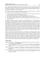
Figure 1.11. Principal results in UET-UCT model for the minimization of the length of the
schedule
With the Figure 1.11, a question arises: " It exists a
-approximation algorithm with INT
for the problems
; and ?"
Moreover, the hierarchical communication delays model is a model more complex as the
homogeneous communication delays model. However, this model is not too complex since
some analytical results were produced.
Scheduling with Communication Delays
81
1.8 Appendix
In this section, we will give some fundamentals results in theory of complexity and
approximation with guaranteed performance. A classical method in order to obtain a lower

for none approximation algorithm is given by the following results called "Impossibility
theorem" (Chrétienne and Picouleau, 1995) and gap technic see (Aussiello et al., 1999).
Theorem 1.8.1 (Impossibility theorem) Consider a combinatorial optimization problem for which
all feasible solutions have non-negative integer objective function value (in particular scheduling
problem). Let c be a fixed positive integer. Suppose that the problem of deciding if there exists a
feasible solution of value at most c is
-complete. Then, for any < (c + l)/c, there does not exist a
polynomial-time
-approximation algorithm A unless = , see ((Chrétienne and Picouleau,
1995), (Aussiello et al, 1999))
Theorem 1.8.2 (The gap technic) Let Q' be an
-complete decision problem and let Q be an NPO
minimization problem. Let us suppose that there exist two polynomial-time computable functions f :
and d : IN and a constant gap > 0 such that, for any instance x of Q'.
Then no polynomial-time r-approximate algorithm for Q with r < 1 + gap can exist, unless
= ,
see (Aussiello et al, 1999).
1.8.1 List of
-complete problems
In this section, some classical .
-complete problems are listed, which are used in this
chapter for the polynomial-time transformation.
problem
Instances: We consider a logic formula with clauses of size two or three, and each positive
literal (resp. negative literal) occurs twice (resp. once). The aim is to find exactly one true
literal per clause. Let n be a multiple of 3 and let be a set of clauses of size 2 or 3. There are
n clauses of size 2 and n/3 clauses of size 3 so that:
• each clause of size 2 is equal to
for some with x y.
• each of the n literals x (resp. of the literals

) for x belongs to one of the n clauses of
size 2, thus to only one of them.
• each of the n literals x belongs to one of the n/3 clauses of size 3, thus to only one of them.
• whenever
is a clause of size 2 for some , then x and y belong to
different clauses of size 3.
We would insist on the fact that each clause of size three yields six clauses of size two.
Question:
Is there a truth assignment for I:
{0,1} such that every clause in has exactly one true
literal?
Clique problem
Instances: Let be G = (V, E) a graph and k a integer.
Question: There is a clique (a complete sub-graph) of size k in G ?
3 - SAT problem
Instances:
• Let be
= {x
1
, , x
n
} a set of n logical variables.
• Let be
= {C
1
, , C
m
} a set of clause of length three: .
Question: There is I: {0,1} a assignment
Multiprocessor Scheduling: Theory and Applications

82
1.8.2 Ratio of approximation algorithm
This value is defined as the maximum ratio, on all instances /, between maximum objective
value given by algorithm h (denoted by (I)) and the optimal value (denoted by (I)),
i.e.
Clearly, we have
.
1.8.3 Notations
The notations of this chapter will precised by using the three fields notation scheme ,
proposed by Graham et al. (Graham et al., 1979):
•
• If
the number of processors is limited,
• If
, then the number of processors is not limited,
• If , then we have unbounded number of clusters constituted by two
processors each,
•
where:
• If
=prec (the precedence graph unspecified
*
• If (the communication delay between to tasks admitting a precedence
constraint is equal to c)
*
• If (the processing time of all the tasks is equal to one).
*
• If =dup (the duplication of task is allowed)
• Si
= . (the duplication of task is not allowed)

•
is the objective function:
• the minimization of the makespan, denoted by C
max
• the minimization of the total sum of completion time, denoted by
where C
j
= t
j
+p
j
1.9 References
Anderson, T., Culler, D., Patterson, D., and the NOW team (1995). A case for
NOW(networks of workstations). IEEE Micro, 15:54–64.
Angel, E., Bampis, E., and Giroudeau, R. (2002). Non-approximability results for the
hierarchical communication problem with a bounded number of clusters. In
B.Monien, R. F., editor, EuroPar’02 Parallel Processing, LNCS, No. 2400, pages 217–
224. Springer-Verlag.
Aussiello, G., Crescenzi, P., Gambosi, G., Kann, V., Marchetti-Spaccamela, A., and Protasi,
M. (1999). Complexity and Approximation, chapter 3, pages 100–102. Springer.
Bampis, E., Giannakos, A., and König, J. (1996). On the complexity of scheduling with large
communication delays. European Journal of Operation Research, 94:252–260.
Bampis, E., Giroudeau, R., and König, J. (2000a). Using duplication for multiprocessor
scheduling problem with hierarchical communications. Parallel Processing Letters,
10(1):133–140.
Scheduling with Communication Delays
83
Bampis, E., Giroudeau, R., and König, J. (2002). On the hardness of approximating the
precedence constrained multiprocessor scheduling problem with hierarchical
communications. RAIRO-RO, 36(1):21–36.

Bampis, E., Giroudeau, R., and König, J. (2003). An approximation algorithm for the
precedence constrained scheduling problem with hierarchical communications.
Theoretical Computer Science, 290(3):1883–1895.
Bampis, E., Giroudeau, R., and König, J C. (2000b). A heuristic for the precedence
constrained multiprocessor scheduling problem with hierarchical communications.
In Reichel, H. and Tison, S., editors, Proceedings of STACS, LNCS No. 1770, pages
443–454. Springer-Verlag.
Bhatt, S., Chung, F., Leighton, F., and Rosenberg, A. (1997). On optimal strategies for cycle-
stealing in networks of workstations. IEEE Trans. Comp., 46:545– 557.
Blayo, E., Debreu, L., Mounié, G., and Trystram, D. (1999). Dynamic loab balancing for
ocean circulation model adaptive meshing. In et al., P. A., editor, Proceedings of
Europar, LNCS No. 1685, pages 303–312. Springer-Verlag.
Blumafe, R. and Park, D. (1994). Scheduling on networks of workstations. In 3d Inter Symp. of
High Performance Distr. Computing, pages 96–105.
Chen, B., Potts, C., and Woeginger, G. (1998). A review of machine scheduling: complexity,
algorithms and approximability. Technical Report Woe-29, TU Graz.
Chrétienne, P. and Colin, J. (1991). C.P.M. scheduling with small interprocessor
communication delays. Operations Research, 39(3):680–684.
Chrétienne, P. and Picouleau, C. (1995). Scheduling Theory and its Applications.
John Wiley & Sons. Scheduling with Communication Delays: A Survey, Chapter 4.
Decker, T. and Krandick, W. (1999). Parallel real root isolation using the descartes method.
In HiPC99, volume 1745 of LNCS. Sringer-Verlag.
Dutot, P. and Trystram, D. (2001). Scheduling on hierarchical clusters using malleable tasks.
In 13th ACM Symposium of Parallel Algorithms and Architecture, pages 199–208.
Garey, M. and Johnson, D. (1979). Computers and Intractability, a Guide to the Theory of NP-
Completeness. Freeman.
Giroudeau, R. (2000). L’impact des délais de communications hiérarchiques sur la complexité et
l’approximation des problèmes d’ordonnancement. PhD thesis, Université d’Évry Val
d’Essonne.
Giroudeau, R. (2005). Seuil d’approximation pour un problème d’ordonnancement en

présence de communications hiérarchiques. Technique et Science Informatique,
24(1):95–124.
Giroudeau, R. and König, J. (2004). General non-approximability results in presence of
hierarchical communications. In Third International Workshop on Algorithms, Models
and Tools for Parallel Computing on Heterogeneous Networks, pages 312–319. IEEE.
Giroudeau, R. and König, J. (accepted). General scheduling non-approximability results in
presence of hierarchical communications. European Journal of Operational Research.
Giroudeau, R., König, J., Moulaï, F., and Palaysi, J. (2005). Complexity and approximation
for the precedence constrained scheduling problem with large communications
delays. In J.C. Cunha, P.M., editor, Proceedings of Europar, LNCS, No. 3648, pages
252–261. Springer-Verlag.
Multiprocessor Scheduling: Theory and Applications
84
Graham, R., Lawler, E., Lenstra, J., and Kan, A. R. (1979). Optimization and approximation
in deterministic sequencing and scheduling theory: a survey. Annals of Discrete
Mathematics, 5:287–326.
Hoogeveen, H., Schuurman, P., and Woeginger, G. (1998). Non-approximability results for
scheduling problems with minsum criteria. In Bixby, R., Boyd, E., and Ríos-
Mercado, R., editors, IPCO VI, Lecture Notes in Computer Science, No. 1412, pages
353–366. Springer-Verlag.
Hoogeveen, J., Lenstra, J., and Veltman, B. (1994). Three, four, five, six, or the complexity of
scheduling with communication delays. Operations Research Letters, 16(3):129–137.
Ludwig, W. T. (1995). Algorithms for scheduling malleable and nonmalleable parallel tasks. PhD
thesis, University of Wisconsin-Madison, Department of Computer Sciences.
Mounié, G. (2000). Efficient scheduling of parallel application : the monotic malleable tasks. PhD
thesis, Institut National Polytechnique de Grenoble.
Mounié, G., Rapine, C., and Trystram, D. (1999). Efficient approximation algorithm for
scheduling malleable tasks. In 11th ACM Symposium of Parallel Algorithms and
Architecture, pages 23–32.
Munier, A. and Hanen, C. (1996). An approximation algorithm for scheduling unitary tasks

on m processors with communication delays. Private communication.
Munier, A. and Hanen, C. (1997). Using duplication for scheduling unitary tasks on m
processors with communication delays. Theoretical Computer Science, 178:119–127.
Munier, A. and König, J. (1997). A heuristic for a scheduling problem with communication
delays. Operations Research, 45(1):145–148.
Papadimitriou, C. and Yannakakis, M. (1990). Towards an architectureindependent analysis
of parallel algorithms. SIAM J. Comp., 19(2):322–328.
Pfister, G. (1995). In Search of Clusters. Prentice-Hall.
Picouleau, C. (1995). New complexity results on scheduling with small communication
delays. Discrete Applied Mathematics, 60:331–342.
Rapine, C. (1999). Algorithmes d’approximation garantie pour l’ordonnancement de tâches,
Application au domaine du calcul parallèle. PhD thesis, Institut National Polytechnique
de Grenoble.
Rosenberg, A. (1999). Guidelines for data-parallel cycle-stealing in networks of workstations I:
on maximizing expected output. Journal of Parallel Distributing Computing, 59(1):31–53.
Rosenberg, A. (2000). Guidelines for data-parallel cycle-stealing in networks of workstations
II: on maximizing guarantee output. Intl. J. Foundations of Comp. Science, 11:183–204.
Saad, R. (1995). Scheduling with communication delays. JCMCC, 18:214–224.
Schrijver, A. (1998). Theory of Linear and Integer Programming. John Wiley & Sons.
Thurimella, R. and Yesha, Y. (1992). A scheduling principle for precedence graphs with
communication delay. In International Conference on Parallel Processing, volume 3,
pages 229–236.
Turek, J., Wolf, J., and Yu, P. (1992). Approximate algorithms for scheduling parallelizable
tasks. In 4th ACM Symposium of Parallel Algorithms and Architecture, pages 323–332.
Veltman, B. (1993). Multiprocessor scheduling with communications delays. PhD thesis, CWI-
Amsterdam, Holland.
5
Minimizing the Weighted Number of Late Jobs
with Batch Setup Times and Delivery Costs on a
Single Machine

George Steiner and Rui Zhang
1
DeGroote School of Business, McMaster University
Canada
1. Introduction
We study a single machine scheduling problem with batch setup time and batch delivery
cost. In this problem, n jobs have to be scheduled on a single machine and delivered to a
customer. Each job has a due date, a processing time and a weight. To save delivery cost,
several jobs can be delivered together as a batch including the late jobs. The completion
(delivery) time of each job in the same batch coincides with the batch completion (delivery)
time. A batch setup time has to be added before processing the first job in each batch. The
objective is to find a batching schedule which minimizes the sum of the weighted number of
late jobs and the delivery cost. Since the problem of minimizing the weighted number of late
jobs on a single machine is already
-hard [Karp, 1972], the above problem is also -
hard. We propose a new dynamic programming algorithm (DP), which runs in
pseudopolynomial time. The DP runs in O(n
5
) time for the special cases of equal processing
times or equal weights. By combining the techniques of binary range search and static
interval partitioning, we convert the DP into a fully polynomial time approximation scheme
(FPTAS) for the general case. The time complexity of this FPTAS is O(n
4
/ + n
4
logn).
Minimizing the total weighted number of late jobs on a single machine, denoted by
[Graham et. al, 1979], is a classic scheduling problem that has been well studied in
the last forty years. Moore [1968] proposed an algorithm for solving the unweighted
problem on n jobs in O(nlogn) time. The weighted problem was in the original list of

-
hard problems of Karp [1972]. Sahni [1976] presented a dynamic program and a fully
polynomial time approximation scheme (FPTAS) for the maximization version of the
weighted problem in which we want to maximize the total weight of on-time jobs. Gens and
Levner [1979] developed an FPTAS solving the minimization version of the weighted
problem in O(n
3
/ ) time. Later on, they developed another FPTAS that improved the time
complexity to O(n
2
logn + n
2
/ ) [Gens and Levner, 1981].
In the batching version of the problem, denoted by
, jobs are processed in batches
which require setup time s, and every job's completion time is the completion time of the
last job in its batch. Hochbaum and Landy [1994] proposed a dynamic programming
algorithm for this problem, which runs in pseudopolynomial time. Brucker and Kovalyov

1
email:,
Multiprocessor Scheduling: Theory and Applications 86
[1996] presented another dynamic programming algorithm for the same problem, which
was then converted into an FPTAS with complexity O(n
3
/ + n
3
logn).
In this paper, we study the batch delivery version of the problem in which each job must be
delivered to the customer in batches and incurs a delivery cost. Extending the classical

three-field notation [Graham et. al., 1979], this problem can be denoted by
bq,
where b is the total number of batches and q is the batch delivery cost. The model, without
the batch setup times, is similar to the single-customer version of the supplier's supply chain
scheduling problem introduced by Hall and Potts [2003] in which the scheduling
component of the objective is the minimization of the sum of the weighted number of late
jobs (late job penalties). They show that the problem is
-hard in the ordinary sense by
presenting pseudopolynomial dynamic programming algorithms for both the single-and
multi-customer case [Hall and Potts, 2003]. For the case of identical weights, the algorithms
become polynomial. However, citing technical difficulties in scheduling late jobs for
delivery [Hall and Potts, 2003] and [Hall, 2006], they gave pseudopolynomial solutions for
the version of the problem where only early jobs get delivered. The version of the problem in
which the late jobs also have to be delivered is more complex, as late jobs may need to be
delivered together with some early jobs in order to minimize the batch delivery costs. In
Hall and Potts [2005], the simplifying assumption was made that late jobs are delivered in a
separate batch at the end of the schedule. Steiner and Zhang [2007] presented a
pseudopolynomial dynamic programming solution for the multi-customer version of the
problem which included the unrestricted delivery of late jobs. This proved that the problem
with late deliveries is also
-hard only in the ordinary sense. However, the algorithm had
the undesirable property of having the (fixed) number of customers in the exponent of its
complexity function. Furthermore, it does not seem to be convertible into an FPTAS. In this
paper, we present for
bq a different dynamic programming algorithm with
improved pseudopolynomial complexity that also schedules the late jobs for delivery.
Furthermore, the algorithm runs in polynomial time in the special cases of equal tardiness
costs or equal processing times for the jobs. This proves that the polynomial solvability of
can be extended to , albeit by a completely different algorithm. We
also show that the new algorithm for the general case can be converted into an FPTAS.

The paper is organized as follows. In section 2, we define the
bq problem in
detail and discuss the structure of optimal schedules. In section 3, we propose our new
dynamic programming algorithm for the problem, which runs in pseudopolynomial time.
We also show that the algorithm becomes polynomial for the special cases when jobs have
equal weights or equal processing times. In the next section, we develop a three-step fully
polynomial time approximation scheme, which runs in O(n
4
/ + n
4
logn) time. The last
section contains our concluding remarks.
2. Problem definition and preliminaries
The problem can be defined in detail as follows. We are given n jobs, J = {1,2, , n}, with
processing time p
j
, weight w
j
, delivery due date . Jobs have to be scheduled
nonpreemptively on a single machine and delivered to the customer in batches. Several jobs
could be scheduled and delivered together as a batch with a batch delivery cost q and
delivery time . For each batch, a batch setup time s has to be added before processing the
first job of the batch. Our goal is to find a batching schedule that minimizes the sum of the
Minimizing the Weighted Number of Late Jobs
with Batch Setup Times and Delivery Costs on a Single Machine
87
weighted number of late jobs and delivery costs. Without loss of generality, we assume that
all data are nonnegative integers.
A job is late if it is delivered after its delivery due date, otherwise it is early. The batch
completion time is defined as the completion time of the last job in the batch on the machine.

Since the delivery of batches can happen simultaneously with the processing of some other
jobs on the machine, it is easy to see that a job is late if and only if its batch completion time
is greater than its delivery due date minus
. This means that each job j has an implied due
date on the machine. This implies that we do not need to explicitly schedule the
delivery times and consider the delivery due dates, we can just use the implied due dates, or
due dates in short, and job j is late if its batch completion time is greater than d
j
. (From this
point on, we use the term due date always for the d
j
.) A batch is called an early batch if all
jobs are early in this batch, it is called a late batch if every job is late in this batch, and a batch
is referred to as mixed batch if it contains both early and late jobs. The batch due date is defined
as the smallest due date of any job in the batch. The following simple observations
characterize the structure of optimal schedules we will search for. They represent
adaptations of known properties for the version of the problem in which there are no
delivery costs and/or late jobs do not need to be delivered.
Proposition 2.1. There exists an optimal schedule in which all early jobs are ordered in EDD
(earliest due date first) order within each batch.
Proof. Since all jobs in the same batch have the same batch completion time and batch due
date, the sequencing of jobs within a batch is immaterial and can be assumed to be EDD.
Proposition 2.2. There exists an optimal schedule in which all late jobs (if any) are scheduled in the
last batch (either in a late batch or in a mixed batch that includes early jobs).
Proof. Suppose that there is a late job in a batch which is scheduled before the last batch in an
optimal schedule. If we move this job into this last batch, it will not increase the cost of the
schedule.
Proposition 2.3. There exists an optimal schedule in which all early batches are scheduled in EDD
order with respect to their batch due date.
Proof. Suppose that there are two early batches in an optimal schedule with batch

completion times t
i
< t
k
and batch due dates d
i
> d
k
. Since all jobs in both batches are early,
we have d
i
> d
k
 t
k
> t
i
. Thus if we schedule batch k before batch i, it does not increase the
cost of the schedule.
Proposition 2.4. There exists an optimal schedule such that if the last batch of the schedule is not a
late batch, i.e., there is at least one early job in it, then all jobs whose due dates are greater than or
equal to the batch completion time are scheduled in this last batch as early jobs.
Proof. Let the batch completion time of the last batch be t. Since the last batch is not a late
batch, there must be at least one early job in this last batch whose due date is greater than or
equal to t. If there is another job whose due date is greater than or equal to t but it was
scheduled in an earlier batch, then we can simply move this job into this last batch without
increasing the cost of the schedule.
Proposition 2.2 implies that the jobs which are first scheduled as late jobs can always be
scheduled in the last batch when completing a partial schedule that contains only early jobs.
The dynamic programming algorithm we present below uses this fact by generating all

possible schedules on early jobs only and designating and putting aside the late jobs, which
get scheduled only at the end in the last batch. It is important to note that when a job is
designated to be late in a partial schedule, then its weighted tardiness penalty is added to
the cost of the partial schedule.
Multiprocessor Scheduling: Theory and Applications 88
3. The dynamic programming algorithm
The known dynamic programming algorithms for do not have a straightforward
extension to
bq, because the delivery of late jobs complicates the matter. We
know that late jobs can be delivered in the last batch, but setting them up in a separate batch
could add the potentially unnecessary delivery cost q for this batch when in certain
schedules it may be possible to deliver late jobs together with early jobs and save their
delivery cost. Our dynamic programming algorithm gets around this problem by using the
concept of designated late jobs, whose batch assignment will be determined only at the end.
Without loss of generality, assume that the jobs are in EDD order, i.e., d
1
 d
2
  d
n
and let
. If d
1
 P + s, then it is easy to see that scheduling all jobs in a single batch will
result in no late job, and this will be an optimal schedule. Therefore, we exclude this trivial
case by assuming for the remainder of the paper that some jobs are due before P + s. The
state space used to represent a partial schedule in our dynamic programming algorithm is
described by five entries {k, b, t, d, v}:
k: the partial schedule is on the job set {1,2, , k}, and it schedules some of these jobs as early
while only designating the rest as late;

b: the number of batches in the partial schedule;
t: the batch completion time of the last scheduled batch in the partial schedule;
d: the due date of the last batch in the partial schedule;
v: the cost (value) of the partial schedule.
Before we describe the dynamic programming algorithm in detail, let us consider how we
can reduce the state space. Consider any two states (k, b, t
1
, d,v
1
) and (k, b, t
2
, d,v
2
). Without
loss of generality, let t
1
t
2
. If v
1
 v
2
, we can eliminate the second state because any later
states which could be generated from the second state can not lead to better v value than the
value of similar states generated from the first state. This validates the following elimination
rule, and a similar argument could be used to justify the second remark.
Remark 3.1. For any two states with the same entries {k,b,t,d, }, we can eliminate the state
with larger v.
Remark 3.2. For any two states with the same entries {k, b, ,d,v}, we can eliminate the state
with larger t.

The algorithm recursively generates the states for the partial schedules on batches of early
jobs and at the same time designates some other jobs to be late without actually scheduling
these late jobs. The jobs designated late will be added in the last batch at the time when the
partial schedule gets completed into a full schedule. The tardiness penalty for every job
designated late gets added to the state variable v at the time of designation. We look for an
optimal schedule that satisfies the properties described in the propositions of the previous
section. By Proposition 2.2, the late jobs should all be in the last batch of a full schedule. It is
equivalent to say that any partial schedule {k, b, t, d, v} with 1  b  n — 1 can be completed
into a full schedule by one of the following two ways:
1. Add all unscheduled jobs {k +1,k + 2, , n} and the previously designated late jobs to
the end of the last batch b if the resulting batch completion time (P + bs) does not exceed
the batch due date d (we call this a simple completion); or
2. Open a new batch b+1, and add all unscheduled jobs {k +1,k + 2, , n} and the
previously designated late jobs to the schedule in this batch. (We will call this a direct
completion.)
Minimizing the Weighted Number of Late Jobs
with Batch Setup Times and Delivery Costs on a Single Machine
89
We have to be careful, however, as putting a previously designated late job into the last
batch this way may make such a job actually early if its completion time (P+bs or P + (b + l)
s, respectively) is not greater than its due date. This situation would require rescheduling
such a designated late job among the early jobs and removing its tardiness penalty from the
cost v. Unfortunately, such rescheduling is not possible, since we do not know the identity
of the designated late jobs from the state variables (we could only derive their total length
and tardy weight). The main insight behind our approach is that there are certain special
states, that we will characterize, whose completion never requires such a rescheduling. We
proceed with the definition of these special states.
It is clear that a full schedule containing exactly l (1  l  n) batches will have its last batch
completed at P + ls. We consider all these possible completion times and define certain
marker jobs m

i
and batch counters
i
in the EDD sequence as follows: Let m
0
be the last job with
< P + s and m
0
+1 the first job with  P+s. If m
0
+1 does not exist, i.e., m
0
= n, then
we do not need to define any other marker jobs, all due dates are less than P + s, and we will
discuss this case separately later. Otherwise, define
0
= 0 and let
1
 1 be the largest integer
for which
 P +
1
s. Let the marker job associated with
1
be the job m
1
 m
0
+ 1 whose
due date is the largest due date strictly less than P + (

1
+1)s, i.e., < P + (
1
+ 1)s and
 P + (
1
+ 1)s. Define recursively for i = 2,3, ,h — 1,
i

i-1
+ 1 to be the smallest counter for
which there is a marker job m
i
m
i-1
+1 such that < P + (
i
+ 1) s and  P+(
i
+ 1) s.
The last marker job is m
h
= n and its counter
h
is the largest integer for which P +
h
s  d
n
<
P + (

h
+ 1)s. We also define
h+1
=
h
+1. Since the maximum completion time to be
considered is P+ns for all possible schedules (when every job forms a separate batch), any
due dates which are greater than or equal to P + ns can be reduced to P + ns without
affecting the solution. Thus we assume that d
n
 P+ns for the rest of the paper, which also
implies
h
+1  n+1.
For convenience, let us also define T
1,0
= P +
1
s, T
i,k
= P + (
i
+ k)s for i = 1, , h and k = 0,1, ,
k(i), where each k(i) is the number for which T
i, k (i)
= P + (
i
+ k(i))s = P +
i+1
s = T

i+1,0
, and T
h,1
= P + (
h
+ l)s. Note that this partitions the time horizon [P, P + (
h
+ l)s] into consecutive
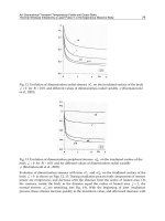
intervals of length s. We demonstrate these definitions in Figure 1.
Figure 1. Marker Jobs and Corresponding Intervals
We can distinguish the following two cases for these intervals:
1. T
i,1
= T
i+1,0
, i.e., k(i) = 1: This means that the interval immediately following I
i
= [T
i,0
, T
i,1
)
contains a due date. This implies that
i+1
=
i
+ 1;
2. T
i,1
T

i+1,0
,i.e., k(i) > 1: This means that there are k(i) — 1 intervals of length s starting at
P + (
i
+ 1)s in which no job due date is located.
In either case, it follows that every job j > m
0
has its due date in one of the intervals I
i
= [T
i,0
, T
i,1
)
for some i {1, , h}, and the intervals [T
i,l
, T
i,l+1
) contain no due date for i = 1, ,h and l>0.
Figure 1 shows that jobs from m
0
+1 to m
1
have their due date in the interval [T
1,0
, T
1,1
). Each
marker job m
i

is the last job that has its due date in the interval I
i
= [T
i,0
, T
i,1
) for i = 1, , h, i.e.,
we have
.
Multiprocessor Scheduling: Theory and Applications 90
Now let us group all jobs into h +1 non-overlapping job sets G
0
= {1, , m
0
}, G
1
= {m
0
+ 1, ,
m
1
} and G
i
= {m
i-1
+ 1, , m
i
} for i = 2, , h. Then we have and i  1. We also
define the job sets J
0

= Go, J
i
= G
0
G
1
G
i
, for i = 1,2, , h — 1 and J
h
= G
0
G
1
G
h
= J.
The special states for DP are defined by the fact that their (k, b) state variables belong to the
set H defined below:
If m
0
= n, then let H = {(n, 1), (n, 2), , (n, n — 1)};
If m
0
< n, then let H = H
1
H
2
H
3

, where
1. If
1
> 1, then H
1
= {(m
0
, 1), (m
0
, 2), , (m
0
,
1
–1)}, otherwise H
1
= ;
2. H
2
= , , , ,
, , ;
3. If 1 <
h
< n, then H
3
= , otherwise H
3
= .
Note that m
h
= n and thus the pairs in H

3
follow the same pattern as the pairs in the other
parts of H. The dynamic program follows the general framework originally presented by
Sahni [1976].
The Dynamic Programming Algorithm DP
[Initialization] Start with jobs in EDD order
1. Set (0, 0, 0, 0, 0)
S
(0)
, S
(k)
= , k = 1, 2, , n, * = , and define m
0
,
i
and m
i
, i = 1,2, , h;
2. If m
0
+ 1 does not exist, i.e., m
0
= n, then set H = {(n, 1), (n, 2), , (n, n — 1)}; Otherwise
set H = H
1
H
2
H
3
.

Let I =
the set of all possible pairs and =I—H , the complementary
set of H.
[Generation] Generate set S
(k)
for k = 1 to n + 1 from S
(k-1)
as follows:
Set = ;
[Operations] Do the following for each state (k — 1,b,t, d, v)inS
(k-1)
Case (k - 1, b)
H
1. If t < P + bs, set
* = * (n, b + 1, P + (b + 1)s, d', v + q) /* Generate the direct
completion schedule and add it to the solution set *, where d' is defined as the due date of
the first job in batch b+ 1;
2. If t = P + bs, set
* = * (n, b, P + bs, d, v) /* We have a partial schedule in which all
jobs are early. (This can happen only when k — 1 = n.)
Case (k - 1, b)
1. If t + p
k
 dandk n, set = (k, b, t + p
k
, d, v) /* Schedule job k as an early job in
the current batch;
2. If t + p
k
+ s  d

k
and k  n, set = (k, b + 1, t + p
k
+ s, d
k
, v + q) /* Schedule job k as
an early job in a new batch;
3. If k  n, set
= (k, b, t, d, v + w
k
) /* Designate job k as a late job by adding its weight
to v and reconsider it at the end in direct completions.
Endfor
[Elimination] Update set S
(k)
1. For any two states (k, b, t, d, v) and (k, b, t, d, v') with v  v', eliminate the one with
v' from set
based on Remark 3.1;
2. For any two states (k, b, t, d, v) and (k, b, t', d, v) with t  t', eliminate the one with t'
from set based on Remark 3.2;
3. Set S
(k)
= .
Endfor
Minimizing the Weighted Number of Late Jobs
with Batch Setup Times and Delivery Costs on a Single Machine
91
[Result] The optimal solution is the state with the smallest v in the set *. Find the optimal
schedule by backtracking through all ancestors of this state.
We prove the correctness of the algorithm by a series of lemmas, which establish the crucial

properties for the special states.
Lemma 3.1. Consider a partial schedule (m
i
, b, t, d, v) on job set J
i
, where (m
i
, b) H. If its
completion into a full schedule has b+1 batches, then the final cost of this completion is exactly v + q.
Proof. We note that completing a partial schedule on b batches into a full schedule on b + 1
batches means a direct completion, i.e., all the unscheduled jobs (the jobs in J — J
i
, if any)
and all the previously designated late jobs (if any) are put into batch b+1, with completion
time P + (b + 1)s.
Since all the previously designated late jobs are from J
i
for a partial schedule (m
i
, b, t, d, v),
their due dates are not greater than
. Therefore, all
designated late jobs stay late when scheduled in batch b+1. Next we show that unscheduled
jobs j
(J — J
i
) must be early in batch b+1. We have three cases to consider.
Case 1. m
0
= n and i = 0:

In this case, H = {(n, 1), (n, 2), , (n,n — 1)} and J
0
= J, i.e. all jobs have been scheduled
early or designated late in the state (m
0
, b, t, d, v). Therefore, there are no unscheduled
jobs.
Case 2.
m
0
< n and b =
i
:
Since
0
= 0 by definition, we must have i  1 in this case. The first unscheduled job j (J
— J
i
) is job m
i
+ 1 with due date . Thus m
i
+1 and all
other jobs from J — J
i
have a due date that is at least P + (b + 1)s, and therefore they will
all be early in batch b+1.
Case 3.
m
0

< n and b >
i
:
This case is just an extension of the case of b =
i
.
If i = 0, then the first unscheduled job for the state (m
0
, b, t, d, v)ism
0
+1. Thus every
unscheduled job j has a due date
, where the last
inequality holds since (m
0
, b) H
i
and therefore, b 
1
— 1.
If 1  i < h, then we cannot have k(i) = 1: By definition, if k(i) =1, then
i
+ k(i)—1 =
i
=
i
+1
—1, which contradicts b >
i
and (m

i
,b) H. Therefore, we must have k(i) > 1, and b
could be any value from {
i
+ 1, ,
i
+ k(i)—1}. This means that P + (b + l)s < P +(
i
+
k(i))s = P +
i+1
s. We know, however, that every unscheduled job has a due date that is
at least T
i+1, 0
= P +
i+1
s. Thus every job from J — J
i
will be early indeed.
If i = h, then we have m
h
= n and J
h
= J, and thus all jobs have been scheduled early or
designated late in the state (m
i
, b, t, d, v). Therefore, there are no unscheduled jobs.
In summary, we have proved that all previously designated late jobs (if any) remain late in
batch b+1, and all jobs from J — J
i

(if any) will be early. This means that v correctly accounts
for the lateness cost of the completed schedule, and we need to add to it only the delivery
cost q for the additional batch b+1. Thus the cost of the completed schedule is v + q indeed.
Lemma 3.2. Consider a partial schedule (m
i
, b, t, d, v) on job set J
i
, where (m
i
, b) H and b n — 1.
Then any completion into a full schedule with more than b + 1 batches has a cost that is at least v + q,
i.e., the direct completion has the minimum cost among all such completions of (m
i
, b,t,d, v).
Proof. If m
i
= n, then the partial schedule is of the form (n, b, t,d,v), (n,b) H, b n — 1. (This
implies that either m
0
= n with i = 0 or (m
i
, b) H
3
with i = h.) Since there is no unscheduled
job left, all the new batches in any completion are for previously designated late jobs. And
since all the previously designated late jobs have due dates that are not greater than
Multiprocessor Scheduling: Theory and Applications 92
, these jobs will stay late in the completion. The number of
new batches makes no difference to the tardiness penalty cost of late jobs. Therefore, the best
strategy is to open only one batch with cost q. Thus the final cost of the direct completion is

minimum with cost v + q.
Consider now a partial schedule (m
i
, b, t, d, v), (m
i
, b) H, b n—1 when m
i
< n. Since all the
previously designated late jobs (if any) are from J
i
, their due dates are not greater than
. Furthermore, since all unscheduled jobs are from J — J
i
, their
due dates are not less than . Thus scheduling all of these jobs
into batch b + 1 makes them early without increasing the tardiness cost. It is clear that this is
the best we can do for completing (m
i
, b, t, d, v) into a schedule with b + 1 or more batches.
Thus the final cost of the direct completion is minimum again with cost v + q.
Lemma 3.3. Consider a partial schedule (m
i
, b, t, d, v} on job set J
i
(i  1), where (m
i
, b) H and b >
1. If it has a completion into a full schedule with exactly b batches and cost v', then there must exist
either a partial schedule
whose direct completion is of the same cost v' or there exists

a partial schedule
whose direct completion is of the same cost v'.
Proof. To complete the partial schedule (m
i
,b,t,d,v) into a full schedule on b batches, all
designated late jobs and unscheduled jobs have to be added into batch b.
Case 1. b >
i
:
Let us denote the early jobs by E
i
J
i
in batch b in the partial schedule (m
i
, b, t, d, v).
Adding the designated late jobs and unscheduled jobs to batch b will result in a batch
completion time of P+bs. This makes all jobs in E
i
late since
for j E
i
. Thus the cost of the full schedule should be . We cannot do this
calculation, however, since there is no information available in DP about what E
i
is. But
if we consider the partial schedule =
with one less batch, where is the smallest due date in batch b — 1 in the
partial schedule (m
i

, b, t, d, v), the final cost of the direct completion of the partial
schedule
would be exactly by
Lemma 3.1. We show next that this partial schedule
does get generated in the algorithm.
In order to see that DP will generate the partial schedule
suppose that during the generation of the partial schedule (m
i
, b, t, d, v), DP starts batch b by
adding a job k as early. This implies that the jobs that DP designates as late on the path of
states leading to (m
i
, b, t, d, v) are in the set L
i
= {k, k + 1, , m
i
}—E
i
. In other words, DP has
in the path of generation for (m
i
,b,t,d,v) a partial schedule .
Then it will also generate from
the partial schedule
by simply designating all jobs in E
i
L
i
as late.
Case 2.

b =
i
1:
Suppose the partial schedule (m
i
, b, t, d, v) has in batch b the sets of early jobs E
i-1
E,
where E
i-1
J
i-1
and E ( J
i
— J
i-1
). Adding the designated late jobs and unscheduled jobs
to batch b will result in a batch completion time of P + bs. This makes all jobs in E
i-1
late
since . On the other hand, if L (J
i
—J
i-1
—E) denotes the
previously designated late jobs from J
i
— J
i-1
in (m

i
, b, t, d, v), then these jobs become
early since
+1
for j L. For similar reasons, all previously designated
late jobs not in L stay late, jobs in E remain early and all other jobs from J — J
i
will be
early too. In summary, the cost for the full completed schedule derived from (m
i
,b,t,d,v)
should be . Again, we cannot do this calculation, since
Minimizing the Weighted Number of Late Jobs
with Batch Setup Times and Delivery Costs on a Single Machine
93
there is no information about E
i-1
and L. However, suppose that E
i-1
, and consider
the partial schedule
=
with one less batch, where d is the smallest due date in batch b — 1 in
the partial schedule (m
i
, b, t, d, v). The final cost of the direct completion of the partial
schedule would be exactly
by Lemma 3.1. Next, we show that this partial schedule
does get generated during the
execution of DP.

To see the existence of the partial schedule =
) note that DP must start batch b on the path of
states leading to (m
i
, b, t, d, v) by scheduling a job k  m
i-1
early in iteration k from a state
(We cannot have k >
m
i-1
since this would contradict E
i-1
. Note also that accounts for the
weight of those jobs from {k, k+l, , m
i-1
} that got designated late between iterations k and m
i-1
during the generation of the state (m
i
,b,t,d,v).) In this case, it is clear that DP will also
generate from a
partial schedule on J
i-1
in which all jobs in E
i-1
are designated late, in addition to those jobs (if
any) from {k, k+1, , m
i-1
} that are designated late in (m
i

, b, t, d, v). Since this schedule will
designate all of {k, k+1, , m
i-1
} late, the lateness cost of this set of jobs must be added, which
results in a state
. This is the state
whose existence we claimed.
The remaining case is when E
i-1
= . In this case, batch b has no early jobs in the partial
schedule (m
i
,b,t,d,v) from the set J
i-1
and if k again denotes the first early job in batch b, then k
J
i
– J
i-1
. This clearly implies that (m
i
,b,t,d,v) must have a parent partial schedule
. Consider the direct completion of this schedule: All designated
late jobs must come from J
i-1
and thus they stay late with a completion time of P + bs.
Furthermore, all jobs from J – J
i-1
will be early, and therefore, the cost of this direct
completion will be .

The remaining special cases of b = 1, which are not covered by the preceding lemma, are (m
i
,
b) = (m
1
, 1) or (m
i
, b) = (m
0
, 1), and they are easy: Since all jobs are delivered at the same time
P + s, all jobs in J
0
or J, respectively, are late, and the rest of the jobs are early. Thus there is
only one possible full schedule with cost
.
In summary, consider any partial schedule (m
i
, b, t, d, v) on job set J
i
, where (m
i
, b) H , or a
partial schedule (n, b, t, d, v) on job set J and assume that the full schedule S' = (n, b' , P + b's,
d' , v') is a completion of this partial schedule and has minimum cost v'. Then the following
schedules generated by DP will contain a schedule among them with the same minimum
cost as S':
1. the direct completion of (m
i
,b,t,d,v), if (m
i

, b) (m
i
,
i
) and b' > b, by Lemma 3.1 and
Lemma 3.2;
2. the direct completion of a partial schedule
, if (m
i
, b) (m
i
,
i
) and b' =
b, by Lemma 3.3;
3. the direct completion of a partial schedule
, if (m
i
, b) = (m
i
,
i
), i > 1 and
b' = b, by Lemma 3.3;
4. the full schedule
if m
0
< n and b'  b =
1
= 1 i.e., (m

i
, b)
= (m
1
, 1);
Multiprocessor Scheduling: Theory and Applications 94
5. the full schedule , if m
0
= n and b'  b = 1. i.e., (m
i
, b) =
(m
0
, 1).
Theorem 3.1. The dynamic programming algorithm DP is a pseudopolynomial algorithm, which
finds an optimal solution for in min time and space,
where
.
Proof. The correctness of the algorithm follows from the preceding lemmas and discussion.
It is clear that the time and space complexity of the procedures [Initialization] and [Result]is
dominated by the [Generation] procedure. At the beginning of iteration k, the total number of
possible values for the state variables {k, b, t, d, v}inS
(k)
is upperbounded as follows: n is the
upper bound of k and b; n is the upper bound for the number of different d values; min{d
n
, P
+ ns} is an upper bound of t and W + nq is an upper bound of v, and because of the
elimination rules, min{d
n

, P+ns, W+nq} is an upper bound for the number of different
combinations of t and v. Thus the total number of different states at the beginning of each
iteration k in the [Generation] procedure is at most O(n
2
min{d
n
, P + ns, W + nq}). In each
iteration k, there are at most three new states generated from each state in S
(k-1)
and this takes
constant time. Since there are n iterations, the [Generations] procedure could indeed be done
in O(n
3
min{d
n
, P + ns, W + nq}) time and space.
Corollary 3.1. For the case of equal weights, the dynamic programming algorithm DP finds an
optimum solution in O(n
5
) time and space.
Proof. For any state, v is the sum of two different cost components: the delivery costs from {q,
2q, , nq} and the weighted number of late jobs from {0, w, , nw}, where w
j
= w, .
Therefore, v can take at most n(n + 1) different values and the upper bound for the number
of different states becomes O(n
3
min{d
n
, P + ns, n

2
}) = O(n
5
).
Corollary 3.2. For the case of equal processing times, the dynamic programming algorithm DP finds
an optimum solution in O(n
5
) time and space.
Proof. For any state, t is the sum of two different time components: the setup times from {s,
,ns} and the processing times from {0,p, ,np}, where p
j
= p, . Thus, t can take at most
n(n + 1) different values, and the upper bound for the number of different states becomes
O(n
3
min{d
n
, n
2
, W + nq}) = O(n
5
).
4. The Fully Polynomial Time Approximation Scheme
To develop a fully polynomial time approximation scheme (FPTAS), we will use static
interval partitioning originally suggested by Sahni [1976] for maximization problems. The
efficient implementation of this approach for minimization problems is more difficult, as it
requires prior knowledge of a lower (LB) and upper bound (UB) for the unknown optimum
value v*, such that the UB is a constant multiple of LB. In order to develop such bounds, we
propose first a range algorithm R(u,
), which for given u and , either returns a full schedule

with cost v  u or verifies that (1 — ) u is a lower bound for the cost of any solution. In the
second step, we use repeatedly the range algorithm in a binary search to narrow the range
[LB, UB] so that UB  2LB at the end. Finally, we use static interval partitioning of the
narrowed range in the algorithm DP to get the FPTAS. Similar techniques were used by
Gens and Levner [1981] for the one-machine weighted-number-of-late-jobs problem
and Brucker and Kovalyov [1996] for the one-machine weighted-number-of-late-
jobs batching problem without delivery costs .
The range algorithm is very similar to the algorithm DP with a certain variation of the
[Elimination] and [Result] procedures.
Minimizing the Weighted Number of Late Jobs
with Batch Setup Times and Delivery Costs on a Single Machine
95
The Range Algorithm R(u, )
[Initialization] The same as that in the algorithm DP.
[Partition] Partition the interval [0, u] into equal intervals of size u /n, with the last one
possibly smaller.
[Generation] Generate set S
(k)
for k = 1 to k = n + 1 from S
(k-1)
as follows:
Set
= ;
[Operations] The same as those in the algorithm DP.
[Elimination] Update set S
(k)
1. Eliminate any state (k, b, t, d, v)ifv > u.
2. If more than one state has a v value that falls into the same interval, then discard all
but one of these states, keeping only the representative state with the smallest t
coordinate for each interval.

3. For any two states (k, b, t, d, v) and (k, b, t, d, v') with v < v', eliminate the one with
v' from set
based on Remark 3.2;
4. Set S
(k)
= .
Endfor
[Result]
If
* = , then v* > (1 - ) u;
If * , then v*  u.
Theorem 4.1. If at the end of the range algorithm R(u,
), we found * = , then v* > (1— )u;
otherwise v*  u. The algorithm runs in O(n
4
/ ) time and space.
Proof. If
* is not empty, then there is at least one state (n, b, t, d, v) that has not been
eliminated. Therefore, v is in some subinterval of [0, u] and v*  v  u. If * = , then all
states with the first two entries (k, b) H have been eliminated. Consider any feasible
schedule (n,b,t,d,v). The fact that
* = means that any ancestor state of (n,b,t,d,v) with cost
must have been eliminated at some iteration k in the algorithm either because > u
or by interval partitioning, which kept some other representative state with cost
' and
maximum error u/n. In the first case, we also have v > u. In the second case,
let v'  ' be the cost of a completion of the representative state and we must have v' > u
since
* = . Since the error introduced in one iteration is at most u/n, the overall error is at
most n( u/n) = u, i.e., v  v'— n( u/n) = v' — u > u — u = (1 — )u. Thus v > (1 — )u for

any feasible cost value v.
For the complexity, we note that
for k = 1,2, ,n. Since all operations on a single
state can be performed in O(1) time, the overall time and space complexity is O(n
4
/ ).
The repeated application of the algorithm R(u,
) will allow us to narrow an initially wide
range of upper and lower bounds to a range where our upper bound is only twice as large
as the lower bound. We will start from an initial range v'  v*  nv'. Next, we discuss how
we can find such an initial lower bound v'.
Using the same data, we construct an auxiliary batch scheduling problem in which we want
to minimize the maximum weight of late jobs, batches have the same batch-setup time s, the
completion time of each job is the completion time of its batch, but there are no delivery
costs. We denote this problem by
. It is clear that the minimum cost of this
problem will be a lower bound for the optimal cost of our original problem.
To solve the problem, we first sort all jobs into smallest-weight-first order,
i.e., w
[1]
 w
[2]
  w
[n]
. Here we are using [k] to denote the job with the kth smallest weight.
Suppose that [k*] has the largest weight among the late jobs in an optimal schedule. It is
Multiprocessor Scheduling: Theory and Applications 96
clear that there is also an optimal schedule in which every job [i], for i = 1,2, , k*, is late,
since we can always reschedule these jobs at the end of the optimal schedule without
making its cost worse. It is also easy to see that we can assume without loss of generality

that the early jobs are scheduled in EDD order in an optimal schedule. Thus we can restrict
our search for an optimal schedule of the following form:
There is a k
{0,1, , n} such that jobs {[k + 1], , [n]} are early and they are scheduled in EDD
order in the first part of the schedule, followed by jobs {[1], [2], , [k]} in the last batch in any
order. The existence of such a schedule can be checked by the following simple algorithm.
The Feasibility Checking Algorithm FC(k)
[Initialization] For the given k value, sort the jobs {[k + 1], , [n]} into EDD order, and let this
sequence be
, where f = n — k.
Set i = 1, j = , t = s + p
j
and d = d
j
lf t > d, no feasible schedule exists and goto [Report];
If t  d, set i = 2 and goto [FeasibilityChecking].
[FeasibilityChecking] While i  f do
Set j =
,
If t + p
j
> d, start a new batch for job j;
if t + s + p
j
> d
j
, no feasible schedule exists and goto [Report};
if t+s+p
j
 d

j
, set t = t+s+p
j
, d = d
j
, i = i+1 and goto [FeasibilityChecking].
If t + p
j
 d, set t = t + p
j
, i = i + 1 and goto [FeasibilityChecking].
Endwhile
[Report]Ifi  f, no feasible schedule exists. Otherwise, there exists a feasible batching
schedule for jobs
in which these jobs are early.
The problem can be solved by repeatedly calling FC(k) for increasing k to
find the first k value, denoted by k*, for which FC(k) returns that a feasible schedule exists.
The Min-Max Weight Algorithm MW
[Initialization] Sort the jobs into a nondecreasing sequence by their weight
w
[1]
 w
[2]
  w
[n]
and set k = 0.
[AlgorithmFC] While k  n call algorithm FC(k).
If FC(k) reports that no feasible schedule exists, set k = k+1 and goto [AlgorithmFC];
Otherwise, set k* = k and goto [Result];
Endwhile

[Result]Ifk* = 0 then there is a schedule in which all jobs are early and set w* = 0; otherwise,
is the optimum.
Theorem 4.2. The Min-Max Weight Algorithm MW finds the optimal solution to the problem
in O(n
2
) time.
Proof. For k = 0, FC(k) constructs the EDD sequence on the whole job set J, which requires
O(nlogn) time. We can obtain the sequence
(f = n — k) in the initialization step of
FC(k + 1), from the sequence constructed for FC(k)inO(n) time by simply deleting
the job [k] from it. It is clear that all other operations in FC(k) need at most O(n) time. Since MW
calls FC(k) at most (n + 1) times, the overall complexity of the algorithm is O(n
2
) indeed.
Corollary 4.1. The optimal solution v* to the problem of minimizing the sum of the weighted number
of late jobs and the batch delivery cost on a single machine,
, is in the interval
[v', nv'], where v' = w* + q.
Proof. It is easy to see that there is at least one batch and there are at most n — k* + 1 batches
in a feasible schedule. Also the weighted number of late jobs is at least w* and at most k*w*
Minimizing the Weighted Number of Late Jobs
with Batch Setup Times and Delivery Costs on a Single Machine
97
in an optimal schedule for . Thus v' = w* + q is a lower bound and k*w* +
(n — k* + 1)q  nw* + nq = n(w* + q) = nv' is an upper bound for the optimal solution v* of
.
Next, we show how to narrow the range of these bounds. Similarly to Gens and Levner [1981],
we use the algorithm R(u, ) with = 1/4 in a binary search to narrow the range [v', nv'].
The Range and Bound Algorithm RB
[Initialization] Set u' = nv'/2;

[BinarySearch] Call R(u', 1/4);
If R(u', 1/4) reports that v*  u', set u' = u' /2 and goto [BinarySearch];
If R(u', 1/4) reports v* > 3 u'/4, set u' = 3u'/2.
[Determination] Call R(u', 1/4).
If R(u', 1/4) reports v*  u', set
= u'/2 and stop;
If R(u', 1/4) reports v* > 3 u'/4, set = 3u'/2 and stop.
Theorem 4.3. The algorithm RB determines a lower bound
for v* such that  v* 2 and it
requires O(n
4
logn) time.
Proof. It can be easily checked that when the algorithm stops, we have  v* 2 . For each
iteration of the range algorithm R(u', 1/4), the whole value interval is divided into
subintervals with equal length
(the last subinterval may be less), where u'  v'. Since only
values v  u' are considered in this range algorithm, the maximum number of subintervals is
less than or equal to . By the proof of Theorem 4.1, the time complexity of
one call to R(u', 1/4) is O(n
4
). It is clear that the binary search in RB will stop after at most
O(logn) calls of R(u', 1/4), thus the total running time is bounded by O(n
4
logn).
Finally, to get an FPTAS, we need to run a slightly modified version of the algorithm DP
with static interval partitioning. We describe this below.
Approximation Algorithm ADP
[Initialization] The same as that in the algorithm DP.
[Partition] Partition the interval [
, 2 ] into equal intervals of size /n, with the last

one possibly smaller.
[Generation] Generate set S
(k)
for k = 1 to k = n + 1 from S
(k-1)
as follows:
Set
= ;
[Operations] The same as those in the algorithm DP.
[Elimination] Update set S
(k)
.
1. If more than one state has a v value that falls into the same sub-interval, then
discard all but one of these states, keeping only the representative state with the
smallest t coordinate.
2. For any two states (k, b, t, d, v) and (k, b, t, d, v') with v  v', eliminate the one with v'
from set
based on Remark 3.2;
3. Set S
(k)
= .
Endfor
[Result] The best approximating solution corresponds to the state with the smallest v over all
states in
*. Find the final schedule by backtracking through the ancestors of this state.
Theorem 4.4. For any > 0, the algorithm ADP finds in O(n
4
/ ) time a schedule with cost v for the
problem, such that v  (1 +
)v*.

Proof. For each iteration in the algorithm ADP, the whole value interval [
, 2 ] is divided
into subintervals with equal length (the last subinterval may be less). Thus the maximum
Multiprocessor Scheduling: Theory and Applications 98
number of the subintervals is less than or equal to . By the proof of Theorem 3.1,
the time complexity of the algorithm is O(n
4
/ ) indeed.
To summarize, the FPTAS applies the following algorithms to obtain an
-approximation for
the problem.
The Fully Polynomial Time Approximation Scheme (FPTAS)
1. Run the algorithm MW by repeatedly calling FC(k) to determine v' = w* + q;
2. Run the algorithm RB by repeatedly calling R(u', 1/4) to determine ;
3. Run the algorithm ADP using the bounds  v*  2 .
Corollary 4.2. The time and space complexity of the FPTAS is O(n
4
logn + n
4
/ ).
Proof. The time and space complexity follows from the proven complexity of the component
algorithms.
5. Conclusions and further research
We presented a pseudopolynomial time dynamic programming algorithm for minimizing the sum
of the weighted number of late jobs and the batch delivery cost on a single machine. For the special
cases of equal weights or equal processing times, the algorithm DP requires polynomial time. We
also developed an efficient, fully polynomial time approximation scheme for the problem.
One open question for further research is whether the algorithm DP and the FPTAS can be
extended to the case of multiple customers.
6. References

P. Brucker and M.Y. Kovalyov. Single machine batch scheduling to minimize the weighted
number of late jobs. Mathematical Methods of Operation Research, 43:1-8, 1996.
G.V. Gens and E.V. Levner. Discrete optimization problems and efficient approximate
algorithms. Engineering Cybernetics, 17(6):1-11, 1979.
G.V. Gens and E.V. Levner. Fast approximation algorithm for job sequencing with
deadlines. Discrete Applied Mathematics, 3(4):313-318, 1981.
R.L. Graham, E.L. Lawler, J.K. Lenstra and A.H.G. Rinnooy Kan. Optimization and
approximation in deterministic sequencing and scheduling: a survey. Ann. Discrete
Math., 4:287-326, 1979.
N.G. Hall and C.N. Potts. The coordination of scheduling and batch deliveries. Annals Of
Operations Research, 135(1):41-64, 2005.
N.G. Hall. Private communication. 2006.
N.G. Hall and C.N. Potts. Supply chain scheduling: Batching and delivery. Operations
Research, 51(4):566-584, 2003.
D.S. Hochbaum and D. Landy. Scheduling with batching: minimizing the weighted number
of tardy jobs. Operations Research Letters, 16:79-86, 1994.
R.M. Karp. Reducibility among combinatorial problem. In R.E. Miller and Thatcher J.W., editors,
Complexity of Computer Computations, pages 85-103. Plenum Press, New York, 1972.
J.M. Moore. An n job, one machine sequencing algorithm for minimizing the number of late
jobs. Management Science, 15:102-109, 1968.
S.K. Sahni. Algorithms for scheduling independent tasks. Journal of the ACM, 23(1): 116-127, 1976.
G. Steiner and R. Zhang. Minimizing the total weighted number of late jobs with late
deliveries in two-level supply chains. 3rd Multidisciplinary International Scheduling
Conference: Theory and Applications (MISTA), 2007.
6
On-line Scheduling on Identical Machines for
Jobs with Arbitrary Release Times
Rongheng Li
1
and Huei-Chuen Huang

2
1
Department of Mathematics, Hunan Normal University,
2
Department of Industrial and Systems Engineering, National University of Singapore
1
China.,
2
Singapore
1. Introduction
In the theory of scheduling, a problem type is categorized by its machine environment, job
characteristic and objective function. According to the way information on job characteristic
being released to the scheduler, scheduling models can be classified in two categories. One
is termed off-line in which the scheduler has full information of the problem instance, such
as the total number of jobs to be scheduled, their release times and processing times, before
scheduling decisions need to be made. The other is called on-line in which the scheduler
acquires information about jobs piece by piece and has to make a decision upon a request
without information of all the possible future jobs. For the later, it can be further classified
into two paradigms.
1. Scheduling jobs over the job list (or one by one). The jobs are given one by one
according to a list. The scheduler gets to know a new job only after all earlier jobs have
been scheduled.
2. Scheduling jobs over the machines' processing time. All jobs are given at their release
times. The jobs are scheduled with the passage of time. At any point of the machines'
processing time, the scheduler can decide whether any of the arrived jobs is to be
assigned, but the scheduler has information only on the jobs that have arrived and has
no clue on whether any more jobs will arrive.
Most of the scheduling problems aim to minimize some sort of objectives. A common
objective is to minimize the overall completion time C
max

, called makespan. In this chapter
we also adopt the same objective and our problem paradigm is to schedule jobs on-line over
a job list. We assume that there are a number of identical machines available and measure
the performance of an algorithm by the worst case performance ratio. An on-line algorithm
is said to have a worst case performance ratio σ if the objective of a schedule produced by
the algorithm is at most σ times larger than the objective of an optimal off-line algorithm for
any input instance.
For scheduling on-line over a job list, Graham (1969) gave an algorithm called List
Scheduling (LS) which assigns the current job to the least loaded machine and showed that
LS has a worst case performance ratio of
where m denotes the number of machines
available. Since then no better algorithm than LS had been proposed until Galambos &
Woeginger (1993) and Chen et al. (1994) provided algorithms with better performance for
Multiprocessor Scheduling: Theory and Applications
100
m 4. Essentially their approach is to schedule the current job to one of the two least loaded
machines while maintaining some machines lightly loaded in anticipation of the possible
arrival of a long job. However for large m, their performance ratios still approach 2 because
the algorithms leave at most one machine lightly loaded. The first successful approach to
bring down the ratio from 2 was given by Bartal et al. (1995), which keeps a constant fraction
of machines lightly loaded. Since then a few other algorithms which are better than LS have
been proposed (Karger et al. 1996, Albers 1999). As far as we know, the current best
performance ratio is 1.9201 which was given by Fleischer & Wahl (2000).
For scheduling on-line over the machines' processing time, Shmoys et al. (1995) designed a
non-clairvoyant scheduling algorithm in which it is assumed any job's processing time is not
known until it is completed. They proved that the algorithm has a performance ratio of 2.
Some other work on the non-clairvoyant algorithm was done by Motwani et al. (1994). On
the other hand, Chen & Vestjens (1997) considered the model in which jobs arrive over time
and the processing time is known when a job arrives. They showed that a dynamic LPT
algorithm, which schedules an available job with the largest processing time once a machine

becomes available, has a performance ratio of 3/2.
In the literature, when job's release time is considered, it is normally assumed that a job
arrives before the scheduler needs to make an assignment on the job. In other words, the
release time list synchronizes with the job list. However in a number of business operations,
a reservation is often required for a machine and a time slot before a job is released. Hence
the scheduler needs to respond to the request whenever a reservation order is placed. In this
case, the scheduler is informed of the job's arrival and processing time and the job's request
is made in form of order before its actual release or arrival time. Such a problem was first
proposed by Li & Huang (2004), where it is assumed that the orders appear on-line and
upon request of an order the scheduler must irrevocably pre-assign a machine and a time
slot for the job and the scheduler has no clue or whatsoever of other possible future orders.
This problem is referred to as an on-line job scheduling with arbitrary release times, which
is the subject of study in the chapter. The problem can be formally defined as follows. For a
business operation, customers place job orders one by one and specify the release time r
j
and the processing time p
j
of the requested job J
j
. Upon request of a customer's job order, the
operation scheduler has to respond immediately to assign a machine out of the m available
identical machines and a time slot on the chosen machine to process the job without
interruption. This problem can be viewed as a generalization of the Graham's classical on-
line scheduling problem as the later assumes that all jobs' release times are zero.
In the classical on-line algorithm, it is assumed that the scheduler has no information on the
future jobs. Under this situation, it is well known that no algorithm has a better performance
ratio than LS for m
3 (Faigle et al. 1989) . It is then interesting to investigate whether the
performance can be improved with additional information. To respond to this question, the
semi-online scheduling is proposed. In the semi-online version, the conditions to be

considered online are partially relaxed or additional information about jobs is known in
advance and one wishes to make improvement of the performance of the optimal algorithm
with respect to the classical online version. Different ways of relaxing the conditions give
rise to different semi-online versions (Kellerer et al. 1997). Similarly several types of
additional information are proposed to get algorithms with better performance. Examples
include the total length of all jobs is known in advance (Seiden et al. 2000), the largest length
of jobs is known in advance (Keller 1991, He et al. 2007), the lengths of all jobs are known in
On-line Scheduling on Identical Machines for Jobs with Arbitrary Release Times
101
[p, rp] where p > 0 and r 1 which is called on-line scheduling for jobs with similar lengths
(He & Zhang 1999, Kellerer 1991), and jobs arrive in the non- increasing order of their
lengths (Liu et al. 1996, He & Tan 2001, 2002, Seiden et al. 2000). More recent publications on
the semi-online scheduling can be found in Dosa et al. (2004) and Tan & He (2001, 2002). In
the last section of this chapter we also extend our problem to be semi-online where jobs are
assumed to have similar lengths.
The rest of the chapter is organized as follows. Section 2 defines a few basic terms and the
LS algorithm for our problem. Section 3 gives the worst case performance ratio of the LS
algorithm. Section 4 presents two better algorithms, MLS and NMLS, for m
2. Section 5
proves that NMLS has a worst case performance ratio not more than 2.78436. Section 6
extends the problem to be semi-online by assuming that jobs have similar lengths. For
simplicity of presentation, the job lengths are assumed to be in [l, r] or p is assumed to be 1.
In this section the LS algorithm is studied. For m
2, it gives an upper bound for the
performance ratio and shows that 2 is an upper bound when . For m = 1, it shows
that the worst case performance ratio is
and in addition it gives a lower bound for
the performance ratio of any algorithm.
2. Definitions and algorithm LS
Definition 1. Let L = {J

1
, J
2
, , J
n
} be any list of jobs, where job J
j
(j = 1, 2, , n) arrives at its
release time r
j
and has a processing time of p
j
. There are m identical machines available.
Algorithm A is a heuristic algorithm.
and denote the makespans of
algorithm A and an optimal off-line algorithm respectively. The worst case performance
ratio of Algorithm A is defined as
Definition 2. Suppose that J
j
is the current job with release time r
j
and processing time p
j
.
Machine M
i
is said to have an idle time interval for job J
j
, if there exists a time interval [T
1

,T
2
]
satisfying the following conditions:
1. Machine M
i
is idle in interval [T
1
,T
2
J and a job has been assigned on M
i
to start processing at time
T
2
.
2. T
2
– max{T
1
, r
j
} p
j
.
It is obvious that if machine M
i
has an idle time interval [T
1
,T

2
] for job J
j
, then job J
j
can be
assigned to machine M
i
in the idle interval.
Algorithm LS
Step 1. Assume that L
i
is the scheduled completion time of machine M
i
(i = 1, 2, ,m).
Reorder machines such that L
1
L
2
L
m
and let J
n
be a new job given to the
algorithm with release time r
n
and running time p
n
.
Step 2. If there exist some machines which have idle intervals for job J

n
, then select a
machine M
i
which has an idle interval [T
1
,T
2
] for job J
n
with minimal T
1
and assign
job J
n
to machine M
i
to be processed starting at time max{T
1
, r
n
} in the idle interval.
Otherwise go to Step 3.
Step 3. Let s = max{r
n
, L
1
}. Job J
n
is assigned to machine M

1
at time s to start the processing.
Multiprocessor Scheduling: Theory and Applications
102
We say that a job sequence is assigned on machine M
i
if starts at its
release time and
starts at its release time or the completion time of ,
depending on which one is bigger.
In the following we let denote the job list assigned on machine
M
i
in the LS schedule and denote the job list assigned on
machine M
i
in an optimal off-line schedule, where (s = 1, 2, , q).
3. Worst case performance of algorithm LS
For any job list L = {J
1
, J
2
, , J
n
}, if r
1
r
2
r
n

, it is shown that R(m, LS) 2 in Hall and
Shmoys(1989). In the next theorem we provide the exact performance ratio.
Theorem 1 For any job list L = {J
1
, J
2
, , J
n
}, if r
1
r
2
r
n
, then we have
(1)
Proof: We will prove this theorem by argument of contradiction. Suppose that there exists
an instance L, called a counterexample, satisfying:
Let L = {J
1
, J
2
, , J
n
} be a minimal counterexample, i.e., a counterexample consisting of a
minimum number of jobs. It is easy to show that, for a minimal counterexample L,
holds.
Without loss of generality we can standardize L such that r
1
= 0. Because if this does not

hold, we can alter the problem instance by decreasing the releasing times of all jobs by r
1
.
After the altering, the makespans of both the LS schedule and the optimal schedule will
decrease by r
1
, and correspondingly the ratio of the makespans will increase. Hence the
altered instance provides a minimal counterexample with r
1
= 0.
Next we show that, at any time point from 0 to
, at least one machine is not idle in
the LS schedule. If this is not true, then there is a common idle period within time interval
[0,
] in the LS schedule. Note that, according to the LS rules and the assumption
that r
1
r
2
r
n
, jobs assigned after the common idle period must be released after this
period. If we remove all the jobs that finish before this idle period, then the makespan of the
LS schedule remains the same as before, whereas the corresponding optimal makespan does
not increase. Hence the new instance is a smaller counterexample, contradicting the
minimality. Therefore we may assume that at any time point from 0 to
at least one
machine is busy in the LS schedule.
As r
1

r
2
r
n
, it is also not difficult to see that no job is scheduled in Step 2 in the LS
schedule.
Now we consider the performance ratio according to the following two cases:
Case 1. The LS schedule of L contains no idle time.
In this case we have
On-line Scheduling on Identical Machines for Jobs with Arbitrary Release Times
103
Case 2. There exists at least a time interval during which a machine is idle in the LS
schedule. In this case, let [a, b] be such an idle time interval with a < b and b being the
biggest end point among all of the idle time intervals. Set
A = {J
j
|J
j
finishes after time b in the LS schedule}.
Let B be the subset of A consisting of jobs that start at or before time a. Let S(J
j
)(j = 1, 2, ,n)
denote the start time of job J
j
in the LS schedule. Then set B can be expressed as follows:
B = {J
j
|b — p
j
< S(J

j
) a}.
By the definitions of A and B we have S(J
j
) > a for any job J
j
A\ B. If both r
j
< b and r
j
< S(J
j
)
hold for some J
j
A \ B, we will deduce a contradiction as follows. Let
be the completion times of M
i
just before job J
j
is assigned in the LS
schedule. First observe that during the period [a, b], at least one machine must be free in the
LS schedule. Denote such a free machine by and let be the machine to which J
j
is
assigned. Then a < S(J
j
)= because r
j
< S(J

j
) and J
j
is assigned by Step 3. On the other hand
we have that
a because r
j
< b and must be free in (a, ) in the LS schedule before
J
j
is assigned as all jobs assigned on machine
to start at or after b must have higher
indices than job J
j
. This implies < and job J
j
should be assigned to machine ,
contradicting the assumption that job J
j
is assigned to machine instead. Hence, for any
job J
j
A \ B, either r
j
b or r
j
= S(J
j
). As a consequence, for any job J
j

A \ B, the
processing that is executed after time b in the LS schedule cannot be scheduled earlier than b
in any optimal schedule. Let = 0 if B is empty and if B is
not empty. It is easy to see that the amount of processing currently executed after b in the LS
schedule that could be executed before b in any other schedule is at most |B|. Therefore,
taking into account that all machines are busy during [b,L
1
] and that |B| m — 1, we obtain
the following lower bound based on the amount of processing that has to be executed after
time b in any schedule:
On the other hand let us consider all the jobs. Note that, if
> 0, then in the LS schedule,
there exists a job J
j
with S(J
j
) a and S(J
j
) – r
j
= . It can be seen that interval [r
j
, S(J
j
)] is a
Multiprocessor Scheduling: Theory and Applications
104
period of time before a with length of , during which all machines are busy just before J
j
is

assigned. This is because no job has a release time bigger than r
j
before J
j
is assigned and, by
the facts that S(J
j
) – r
j
= > 0, and . Combining with the
observations that during the time interval [b, L
1
] all machines are occupied and at any other
time point at least one machine is busy, we get another lower bound based on the total
amount of processing:
Adding up the two lower bounds above, we get
Because r
n
b, we also have
Hence we derive
Hence we have
. This creates a contradiction as L is a counterexample
satisfying
. It is also well-known in Graham (1969) that, when r
1
= r
2
=
= r
n

= 0, the bound is tight. Hence (1) holds.
However, for jobs with arbitrary release times, (1) does not hold any more, which is stated in
the next theorem.
Theorem 2. For the problem of scheduling jobs with arbitrary release times,
Proof: Let L = { J
1
, J
2
, , J
n
} be an arbitrary sequence of jobs. Job J
j
has release time r
j
and
running time p
j
(j = 1, 2, ,n). Without loss of generality, we suppose that the scheduled
completion time of job J
n
is the largest job completion time for all the machines, i.e. the
makespan. Let P be , u
i
(i
=
1, 2, , m) be the total idle time of machine M
i
, and s be
the starting time of job J
n

. Let u = s — L
1
, then we have
It is obvious that