Multiprocessor Scheduling Part 10 docx
Bạn đang xem bản rút gọn của tài liệu. Xem và tải ngay bản đầy đủ của tài liệu tại đây (366.95 KB, 30 trang )
Multiprocessor Scheduling: Theory and Applications
260
job k in stage i are the same, because the corresponding processor in stage i+1 is idle at the
same time and job l can be processed on stage i+1 immediately after completion in stage i.
Figure 1. A flexible flow line with no intermediate buffers
Figure 2. A schema of processor blocking
As noted earlier, setup time can include the time for preparing the machine or the processor.
In an FFLPB with sequence-dependent setup time (FFLPB-SDST), it is assumed that the
setup time depends on both jobs to be processed, the immediately preceding job, and the
corresponding stage. Thus, a proper operation sequence on the processors has a significant
effect on the makespan (i.e., C
max
). As already assumed, the processors in each stage are
identical, whereas the stages are different. Therefore, it is assumed that the setup time also
depends on the stage type. A schema of sequence-dependent setup time in the FFLPB is
illustrated in Figure 4. Job q must be processed immediately before job k in stage i. Also, job l
must be processed immediately before job k in stage i+1. s
iqk
is equal to the processor setup
time for job k if job q is the immediately preceding job in the sequence operation on the
corresponding processor. Likewise, s
(i+1)lk
is equal to the processor setup time for job k if job l
is the immediately preceding job. Job q is completed in stage i at time c
iq
and departs as time
d
iq
t c
iq
to an available processor in stage i+1 (excepting the one that is processing job k). As a
result, job k is started at time d
iq
+s
iqk
in stage i and departs at time d
ik
t d
(i+1)l
to stage i+1.
Likewise, job l is completed in stage i+1 at time c
(i+1)l
and departs at time d
(i+1)l
t c
(i+1)l
to an
available processor in the next stage. As a result, job k started at time d
(i+1)l
+s
(i+1)lk
in stage
1
2
n
1
Sta
g
e 1
1
2
n
2
1
2
n
m
Sta
g
e mSta
g
e 2
k
k
0
Processor blockin
g
d
ik
c
(i+1)k
c
ik
p
ik
p
(i+1)k
Wait
time
Sta
g
e
Sta
g
e i
Sta
g
e i+1
Time
A New Mathematical Model for Flexible Flow Lines with Blocking Processor and
Sequence-Dependent Setup Time
261
i+1 and completed at time c
(i+1)k
. It is worth noting that the blocking processor or idle times
cannot be used as setup time, because we assume the preparing processor requires the
presence of a job.
k
Stage i
Stage i+1
k
0
Sta
g
e
c
(
i+1
)
k
l
d
ik
c
ik
= d
ik
p
ik
p
(
i+1
)
k
Idle
time
Time
c
(
i+1
)
l
d
(
i+1
)
l
Figure 3. A schema of idle time
Figure 4. A schema of sequence-dependent setup time in FFLPB
4. Problem Formulation
In this section, we present a proposed model for the FFLP by considering both the blocking
processor and sequence-dependent setup time. This model belongs to the mixed-integer
nonlinear programming (MINLP) category. Then, we present a linear form for the proposed
model. Without loss of generality, the FFLP can be modeled based on a traveling salesman
k
Stage i
Stage i+1
k
Sta
g
e
d
ik
d
ik
Time
0
d
iq
c
ik
q
l
d
iq
s
iqk
c
iq
s
(
i
+1)
lk
c
(
i
+1)
1
d
(
i
+1)
1
Multiprocessor Scheduling: Theory and Applications
262
problem approach (TSP), since each processor at each stage plays the role of salesman once
jobs (nodes) have been assigned to the processor. In this case, the sum of setup time and
processing time indicates the distance between nodes. Thus, essentially the FFLP is an NP-
hard problem (Kurz and Askin, 2004). A detailed breakdown of the proposed model
follows.
4.1. Assumptions
The problem is formulated under the following assumptions. Like Kurz and Askin (2004),
we also consider blocking processor and sequence-dependent setup times.
1. Machines are available at all times, with no breakdowns or scheduled or unscheduled
maintenance.
2. Jobs are always processed without error.
3. Job processing cannot be interrupted (i.e., no preemption is allowed) and jobs have no
associated priority values.
4. There is no buffer between stages, and processors can be blocked.
5. There is no travel time between stages; jobs are available for processing at a stage
immediately after departing at previous stage.
6. The ready time for all jobs is zero.
7. Machines in parallel are identical in capability and processing rate.
8. Non-anticipatory sequence-dependent setup times exist between jobs at each stage.
After completing processing of one job and before beginning processing of the next job,
some sort of setup must be performed.
4.2. Input Parameters
m = number of processing stage.
K = number of jobs.
n
i
= number of parallel processors in stage i.
p
ik
= processing time for job k in stage i.
s
ilk
= processor setup time for job k if job l is the immediately preceding job in sequence
operation on the processor i. As discussed earlier, we assume that processors at each
stage are identical, thus S
ilk
is independent of index j, i.e., the processor index.
4.3. Indices
i = processing stage, where i =1,…, m.
j = processor in stage, where j =1,…, n
i
.
k, l = job, where k, l =1,…, K.
4.4. Decision Variables
C
max
= makespan.
c
ik
= completion time of job k at stage i.
d
ik
= departure time of job k from stage i.
x
ijlk
= 1, if job k is assigned to processor j in stage i where job l is its predecessor job;
otherwise x
ijlk
= 0. Two nominal jobs 0 and K+1 are considerd as the first and last
jobs, respectively (Kurz and Askin, 2004). It is assumed that nominal jobs 0 and
K+1 have zero setup and process time and must be processed on each processor in
each stage.
A New Mathematical Model for Flexible Flow Lines with Blocking Processor and
Sequence-Dependent Setup Time
263
4.5. Mathematical Formulation
Min C
max
s.t.
10,
1 ,
i
n
K
ijlk
jllk
x
ik
z
¦¦
(1)
1
0, 1,
, ,
KK
ijlk ijkq
llk qqk
x
xi
z z
¦¦
jk
k
(2)
(3)
11 100
1
i
n
kk jkik
j
cp xs
t
¦
(4)
(-1)
10
- 1,
i
n
K
ik i k ik ijlk ilk
jl
cc p xs i k
t !
¦¦
(5)
10,
, 1, , 1
i
n
K
ik ik ijlk ilk il
jllk
cp xsd ik K
z
t
¦¦
(6)
(1)
10,
1,
i
n
K
ik i k ik ijlk ilk
jllk
cd p xs i k
z
!
¦¦
c
mk
=d
mk
k (7)
C
max
t c
mk
k (8)
x
ijlk
{0,1} i,j,l,k ; c
ik
, d
ik
t 0 i,k
The objective function is to minimize the schedule length. Constraint (1) ensures that each
job k in every stage is assigned to only one processor immediately after job l. Constraint (2),
which is complementary to Constraint (1), is a flow balance constraint, guaranteeing that
jobs are performed in well-defined sequences on each processor at each stage. This
constraint determines which processors at each stage must be scheduled. Constraint (3)
calculates the complete time for the first available job on each processor at stage 1. Likewise,
Constraint (4) calculates the complete time for the first available job on each processor in
other stages, and also guarantees that each job is processed in all downstream stages with
regard to setup time related to both the job to be processed and the immediately preceding
job. Constraint (5) controls the formation of the processor's blocking. Constraint (6)
calculates the processing of a job depending on the processing of its predecessor on the same
processor in a given stage. This constraint controls creating the processor's idle time. Both
constraint sets (5) and (6) ensure that a job cannot begin setup until it is available (done at
the previous stage) and the previous job at the current stage is complete. Constraint (6)
indicates that the processing of each job in every stage starts immediately after its departure
from the previous stage plus the setup time of the immediately preceding job. Actually, this
constraint calculates the departure time related to each job at each stage except for the last
stage. Constraint (7) ensures that each product leaves the line as soon as it is completed in
the latest stage. Finally, Constraint (8) defines the maximum completion time.
Multiprocessor Scheduling: Theory and Applications
264
4.6. Model Linearization
The proposed model has a nonlinear form because of the existence of Constraint (5). Thus, it
cannot be solved optimally in a reasonable time by programming approaches. Thus, we
present a linear form for the proposed model by defining the integer variable y
ijlk
and
changing Constraint (5), as indicated in the following expressions.
1 , , ,
ijlk ilk il ijlk
ysdM x ijltu k
(9)
(10)
11,
,
i
n
K
ik ik ijlk
jllk
cp y ik
z
t
¦¦
where M is an arbitrary big number. Constraint (5) must be replaced by Constraints (9) and
(10) in the above proposed model.
4.7 A Lower Bound for the Makespan
In this section, we develop a processor based on a lower bound and evaluate schedules
produced in this manner with other heuristic (or metaheuristic) approaches. The proposed
lower bound was developed based on the lower-bound method presented by Sawik (2001)
for the FFLPB. The proposed lower bound resulted from the following theorem:
Theorem. Equation (11) is the lower bound on any feasible solution of the proposed model.
^` ^`
1
11
1
11 1
max min min
Ki m
mKK
ik ik
hk hk hk hk
kk
i
kh hi
i
pS
LB p S p S
n
½
®¾
¯¿
¦¦ ¦
(11)
where,
^`
1
min ,
K
ik ilk
l
Ss
ik
Proof. Let S
ik
be the minimum time required to set up job k at stage i. We know that every
job k must be processed at each stage and must also be set up. In an optimistic case, we
assume that the work-load incurred to processors at each stage is identical. Thus, each
processor at stage i has the minimum mean workload (1/n
i
)u(¦
k
[p
ik
+S
ik
]) (i.e., the first term
in Equation (11)). According to constraint sets (4) and (5), a job cannot begin setup until it is
available and the previous job at the current stage is complete. Actually, constraint sets (4)
and (5) remark two facts. First, each processor at each stage i incurs an idle time because of
waiting for the first available job. A lower bound for this waiting time in stage i can be the
second term in Equation (11). Second, each processor at each stage i incurs an idle time after
accomplishment of processing untill the end of scheduling. This idle time is equal to the
sum of the minimum time to processing jobs at the next stages (i.e., i+1, , m). A lower
bound for this idle time can be the third term in Equation (11). The sum of the above three
terms indicates a typical lower bound in terms of an optimistic scheduling in stage i. Thus,
LB in Equation (11) is a lower bound on any feasible solution.
5. Numerical Examples
In this section, many numerical examples are presented, and some computational results are
reported to illustrate the efficiency of the proposed approach. Fourteen small-sized
problems are considered in order to evaluate the proposed model. Each problem has some
integer processing times selected from a uniform distribution between 50 and 70, and
A New Mathematical Model for Flexible Flow Lines with Blocking Processor and
Sequence-Dependent Setup Time
265
integer setup times selected from a uniform distribution between 12 and 24 (Kurz and
Askin, 2004). To verify the model and illustrate the approach, problems were generated in
the following three categories: (1) Classical flow shop (one processor at each stage), termed
CAT1 problems; (2) FFLP with the same number of processors at each stage, termed CAT2
problems; and (3) FFLP with a different number of processors at each stage, termed CAT3
problems. The CAT1 problems are considered simply to verify the performance of the
proposed model. To make the comparison of runs simpler and also for standardization, we
assume that the total number of processors in all stages is equal to double the number of
stages, i.e., ¦
k
n
k
= 2um. For example, a problem with three stages has six processors in total.
These problems have been solved by the Lingo 8.0 software on a personal computer with
Celeron M 1.3 GHz CPU and 512 MB of memory. Each problem is allowed a maximum of
7200 seconds of CPU time (two hours) using the Lingo setting (o/Option/General
Solver/time Limitation = 7200 Sec.).
Table 1 contains additional information about CAT1 problems for finding optimal solutions
(i.e., classical flow shop). Problems are considered with two, three, and four stages and more
than four jobs. The values for Columns 'B/B Steps' and 'CPU Time' are two vital criteria for
measuring the severity and complexity of the proposed model. Also, the dimension of the
problem is shown when regarding the number of 'Variables' and 'Constraints' in Table 1. In
CAT1 problems, the number of variables is less than the number of constraints. Thus, CAT1
problems are more severe than CAT2 and CAT3 problems in terms of the time complexity and
computational time required. For example, despite all efforts, a feasible solution is not found in
2 hours for problem 10 (i.e., 6 jobs and 4 stages = 4 processors). However, for problem 3 in
Table 2 with nearly the same condition and dimension (i.e., 6 jobs and 2 stages = 4 processors),
the optimal solution is reached in less than one hour. Likewise, for problem 3 in Table 3 (i.e., 6
jobs and 2 stages = 4 processors), the optimal solution is reached in less than three minutes. To
illustrate the complexity of solving FFLPB-SDST, the behavior of the B/B’s CPU time vs.
increasing the number of jobs for different numbers of stages related to data provided in Table
1 is shown in Figure 5. As the figure indicates, by increasing the number of stages, the CPU
time increases progressively. Table 1 also shows that increasing the number of stages (or
processors) leads to a greater increase in computational time, rather than an increase in the
number of jobs. Table 2 contains additional problem characteristics and information for
optimal solutions related to CAT2 problems (i.e., there are two processors at each stage).
Likewise, Table 3 contains additional problem information for obtaining optimal solutions
related to CAT3 problems (i.e., different numbers of processors at each stage).
Number of
No.
Km n
i
Variables Constraints B/B Steps CPU Time
C
max
LB
1 4 2 1,1 81 95 330 00:00:03 384 383
2 5 2 1,1 121 138 2743 00:00:17 450 445
3 6 2 1,1 169 189 151739 00:14:52 524 503
4 7 2 1,1 225 248 - > 2 hours 610* 585
5 4 3 1,1,1 121 140 1849 00:00:25 465 430
6 5 3 1,1,1 181 204 9588 00:01:45 544 519
7 6 3 1,1,1 253 280 - > 2 hours 615* 577
8 4 4 1,1,1,1 161 185 297 00:00:26 548 520
9 5 4 1,1,1,1 241 270 122412 00:21:20 627 605
10 6 4 1,1,1,1 337 371 - > 2 hours Infeasible** 700
* The best feasible objective value is found so far.
** A feasible solution is not found so far.
Table 1. Optimal solutions for CAT1 problems
Multiprocessor Scheduling: Theory and Applications
266
Number of
No.
Km n
i
Variables Constraints B/B Steps CPU Time
C
max
LB
1 4 2 2,2 145 145 872 00:00:05 230 218
2 5 2 2,2 221 220 10814 00:00:55 295 252
3 6 2 2,2 313 311 240586 00:47:36 299 291
4 7 2 2,2 421 418 - > 2 hours 380* 335
5 4 3 2,2,2 217 215 6644 00:00:32 314 306
6 5 3 2,2,2 331 327 232987 01:02:38 376 328
7 6 3 2,2,2 469 463 - > 2 hours 389* 376
8 4 4 2,2,2,2 289 285 28495 00:02:23 395 392
9 5 4 2,2,2,2 441 434 - > 2 hours 446* 390
* The best feasible objective value is found so far.
Table 2. Optimal solution for CAT2 problems
Number of
No.
Km n
i
Variables Constraints B/B Steps CPU Time
C
max
LB
1 4 2 1,3 209 145 251 00:00:03 381 380
2 5 2 1,3 321 220 1849 00:00:36 434 429
3 6 2 1,3 457 311 6921 00:02:32 527 523
4 7 2 1,3 617 418 - > 2 hours 584* 577
5 4 3 2,1,3 311 215 754 00:00:11 437 426
6 5 3 2,1,3 481 327 89714 00:13:52 484 479
7 6 3 2,1,3 685 463 84304 00:25:26 574 570
8 7 3 2,1,3 925 623 - > 2 hours 645* 639
* The best feasible objective value is found so far.
Table 3. Optimal solution for CAT3 problems
m=3
m=2
m=1
Figure 5. The behavior of the B/B’s CPU time vs. increasing the number of jobs for a
different number of stages
A linear regression analysis was made to fit a line through a set of observations related to
values of C
max
(i.e., makespan) vs. the lower bound (LB). Original figures were obtained
from the results in Tables 1, 2, and 3. This analysis can be useful for estimating the C
max
value for the large-sized problems genererated by using the form presented in this chapter.
A New Mathematical Model for Flexible Flow Lines with Blocking Processor and
Sequence-Dependent Setup Time
267
A scatter diagram of C
max
vs. the LB is shown in Figure 5. Obviously, the linear trend of the
scatter diagram is noticeable. Table 4 contains regression results. According to Table 4, C
max
can be estimated as . The R
2
value, which is called the coefficient of
determination, compares estimated with actual C
max
values ranging from 0 to 1. If R
2
is 1,
then there is a perfect correlation in the sample and there is no difference between the
estimated C
max
value and the actual C
max
value. At the other extreme, if R
2
is 0, the regression
equation is not helpful in predicting a C
max
value. Thus, R
2
= 0.981 implies the goodness of
fitness and observations. For instance, we generate a problem with 20 jobs and 3 stages
belonging to CAT2 (two processors at each stage) that cannot be solved optimally in a
reasonable time. According to Equation (14), the lower bound for the generated problem is
886, thus, the estimated C
max
is 893. If some other approach can achieve a solution with a
C
max
value in the interval (886, 893], we can say that this is an efficient approach. Thus,
interval (LB, ] can be a proper criterion for evaluating the performance of other
approaches.
max
ˆ
C 0.9833 LB 0.0325 u
max
ˆ
C
Slop Constant
R
2
Regression sum of squares Residual sum of squares
0.9833 0.0325 0.981 912.44 202313.79
Table 4. Regression results
As further illustrations, we present a typical optimal scheduling for each category of
problem, i.e., CAT1, CAT2, and CAT3, in Figures 7, 8, and 9, respectively. These figures are
created by using the notations shown in Figure 6. Figure 7 illustrates the optimal scheduling
for problem 9 in Table 1. For instance, there is a blocking time in stage 2 (S2-P2), that is close
to the completion time of job 3, since job 2 is not departed from stage 3. In addition, there is
a blocking processor and immediate idle time in stage 3 that is close to the completion time
of job 3, because job 2 is not still departed from stage 4 and the completion time of job 1 in
stage 2 is greater than departure time of job 3 in stage 3. It is worth noting that the
processing sequence is the same at all stages implying a classical flow shop. Figure 8 depicts
the optimal scheduling for problem 6 shown in Table 2, in which there is one tiny blocking
time and several relatively long idle times. For instance, there is a tiny blocking time next to
job 3 in stage 2 on processor 1 (S2-P1) because job 2 is not yet departed from stage 3 on
processor 2 (S3-P2). Figure 8 also presents the processing sequence between each pair of
observed jobs. For example, the departure time of job 2 is always later than the setup time
(processing start time) of job 1 at the stages. In general, we expect few blocking times for
CAT1 and CAT2 problems because there are an equal number of processors at each stage
and the model endeavors to allocate the same workload to each processor at each stage for
minimizing C
max
. On the other hand, in CAT3 problems, we expect more blocking time
because of the unequal number processor times at each stage. For instance, as shown in
Figure 9, there are two relatively long blocking times in stage 1 because all jobs must be
processed in stage 2 on only one processor. On the other hand, there are several relatively
long idle times in stage 3 because of the above reason. Actually, stage 2 plays the role of
bottleneck here.
Multiprocessor Scheduling: Theory and Applications
268
0
100
200
300
400
500
600
700
Cmax
Figure 5.
C
max
vs. the lower bound (LB)
Tiny idle
time
Tiny
blocking
Departure
time
Setup time Blocking Idle time
Figure 6. Legends
Figure 7. Optimal scheduling for problem 9 shown in Table 1 from CAT1
A New Mathematical Model for Flexible Flow Lines with Blocking Processor and
Sequence-Dependent Setup Time
269
Figure 8. Optimal scheduling for problem 6 shown in Table 2 from CAT2
Figure 9. Optimal scheduling for problem 6 shown in Table 2 from CAT3
Multiprocessor Scheduling: Theory and Applications
270
6. Conclusions
In this chapter, we presented a new mixed-integer programming approach to the flexible
flow line problem without intermediate buffers by assuming in-process buffers and
sequence-dependent setup time. The proposed mathematical model can provide an optimal
schedule by considering blocking processor and idle time as well as sequence-dependent
setup time. We solved the proposed model for three problem categories, i.e., classical flow
shop (CAT1), stages with an equal number of processors (CAT2), and stages with an
unequal number of processors (CAT3). Computation results showed that solving CAT3
problems requires low computational time, since there are less complex than CAT1 and
CAT2 problems. On the other hand, in the classical flow shop case (i.e., CAT1), a high
computational time is required. In many practical situations, the proposed model cannot
optimally solve more than seven jobs with three stages (or six processors). Further, we
developed a lower bound to evaluate the schedules produced with other heuristic or
metaheuristic approaches. Also, a linear regression analysis was made to find a logical
relationship between the makespan and its lower bound, which can be used in future
research. The proposed model can be solved by other heuristic or metaheuristic approaches
as well, and with uncertain processing times and/or setup times. It can also be solved using
limited intermediate buffers instead of in-process buffers.
7. References
Alisantoso, D.; Khoo, L.P. & Jiang, P.Y. (2003). An immune algorithm approach to the
scheduling of a flexible PCB flow shop. Int. J. of Advanced Manufacturing Technology,
Vol. 22, pp. 819-827.
Allahverdi, A.; Gupta, J. & Aldowaisan, T. (1999). A review of scheduling research involving
setup considerations. Omega, Int. J. Mgmt Sci., Vol. 27, pp. 219-239.
Blazewicz, J.; Ecker, K.H.; Schmidt, G. & Weglarz, J. (1994). Scheduling in Computer and
Manufacturing Systems. Berlin: Springer-Verlag.
Bianco, L.; Ricciardelli; S.; Rinaldi, G. & Sassano, A. (1988). Scheduling tasks with sequence-
dependent processing times. Naval Res. Logist, Vol. 35, pp. 177-84.
Bitran, G.R. & Gilbert, S.M. (1990). Sequencing production on parallel machines with two
magnitudes of sequence-dependent setup cost. J. Manufact Oper Manage, Vol. 3, pp.
24-52.
Botta-Genoulaz, V. (2000). Hybrid flow shop scheduling with precedence constraints and
time lags to minimize maximum lateness. Int. J. of Production Economics, Vol. 64,
Nos. 1–3, pp. 101–111.
Brandimarte, P. (1993). Routing and scheduling in a flexible job shop by tabu search. Annals
of Operations Research, Vol. 41, pp. 157-183.
Conway, R.W.; Maxwell, W.L. & Miller, L.W. (1967). Theory of Scheduling, Addison Wesley,
MA.
Daniels, R.L. & Mazzola, J.B. (1993). A tabu-search heuristic for the flexible-resource flow
shop scheduling problem. Annals of Operations Research, Vol. 41, pp. 207-230.
Das, S.R.; Gupta, J.N.D. & Khumawala, B.M. (1995). A saving index heuristic algorithm for
flowshop scheduling with sequence dependent setup times. J. Oper Res Soc, Vol. 46,
pp. 1365-73.
A New Mathematical Model for Flexible Flow Lines with Blocking Processor and
Sequence-Dependent Setup Time
271
Franca, P.M.; Gendreau, M.; Laporte, G. & Muller, F.M. (1996). A tabu search heuristic for
the multiprocessor scheduling problem with sequence dependent setup times. Int J.
Prod Econ, Vol. 43, pp. 79-89.
Flynn, B.B. (1987). The effects of setup time on output capacity in cellular manufacturing.
Int. J. Prod Res, Vol. 25, pp. 1761-72.
Greene, J.T. & Sadowski, P.R. (1986). A mixed integer program for loading and scheduling
multiple flexible manufacturing cells. European Journal of Operation Research, Vol. 24,
pp. 379-386.
Hall, N.G. & Sriskandarajah, C. (1996). A survey of machine scheduling problems with
blocking and no-wait in process. Operations Research, Vol. 44, pp. 510-525.
Hong, T P.; Wang, T T. & Wang, S L. (2001). A palmer-based continuous fuzzy flexible
flow-shop scheduling algorithm. Soft Computing, Vol. 6., pp. 426-433.
Jayamohan, M.S. & Rajendran, C. (2000). A comparative analysis of two different
approaches to scheduling in flexible flow shops. Production Planning & Control,
2000, Vol. 11, No. 6, pp. 572-580.
Jiang, J. & Hsiao, W. (1994). Mathematical programming for the scheduling problem with
alterative process plan in FMS. Computers and Industrial Engineering, Vol. 27, No. 10,
pp. 5-18.
Jungwattanakit, J.; Reodecha, M.; Chaovalitwongse, P. & Werner, F. (2007). Algorithms for
flexible flow shop problems with unrelated parallel machines, setup times, and
dual criteria. Int. J. of Advanced Manufacturing Technology, DOI 10.1007/s00170-007-
0977-0.
Kaczmarczyk, W., Sawik, T., Schaller, A. and Tirpak T.M. (2004). Optimal versus heuristic
scheduling of surface mount technology lines. Int. J. of Production Research, Vol. 42,
No. 10, pp. 2083-2110.
Kim, S.C. & Bobrowski, P.M. (1994). Impact of sequence-dependent setup times on job shop
scheduling performance. Int. J. Prod Res., Vol. 32, pp. 1503-20.
Kis, T. & Pesch, E. (2005). A review of exact solution methods for the non-preemptive
multiprocessor flowshop problem. Eur. J. of Operational Research, Vol. 164, No. 3, pp.
592-608.
Krajewski, L.J.; King, B.E.; Ritzman, L.P. & Wong, D.S. (1987). Kanban, MRP, and shaping
the manufacturing environment. Manage Sci, Vol. 33, pp. 39-57.
Kurz, M.E. & Askin, R.G. (2004). Scheduling flexible flow lines with sequence-dependent
setup times. Eur. J. of Operational Research, Vol. 159, pp. 66–82.
Kusiak, A. (1988). Scheduling flexible machining and assembly systems. Annals of Operations
Research, Vol. 15, pp. 337-352.
Lee, C Y. & Vairaktarakis, G.L. (1998). Performance comparison of some classes of flexible
flow shops and job shops. Int. J. of Flexible Manufacturing Systems, Vol. 10, pp. 379-
405.
McCormick, S.T.; Pinedo, M.L.; Shenker, S. & Wolf, B. (1989). Sequencing in an assembly line
with blocking to minimize cycle time. Operation Research, Vol. 37, pp. 925-936.
Ovacik, I.M. & Uzsoy, R.A. (1992). Shifting bottleneck algorithm for scheduling
semiconductor testing operations. J. Electron Manufact, Vol. 2, pp. 119-34.
Panwalkar, S.S.; Dudek, R.A. & Smith, M.L. (1973). Sequencing research and the industrial
scheduling problem. In: Symposium on the Theory of Scheduling and its Applications,
Elmaghraby, S.E. (editor), pp. 29-38.
Multiprocessor Scheduling: Theory and Applications
272
Pinedo, M. (1995), Scheduling: Theory, Algorithms, and Systems. Prentice Hall, NJ.
Quadt, D. & Kuhn, H. (2005). Conceptual framework for lot-sizing and scheduling of
flexible flow lines. Int. J. of Production Research, Vol. 43, No. 11, pp. 2291-2308.
Quadt, D. & Kuhn, H. (2007). A taxonomy of flexible flow line scheduling procedures. Eur. J.
of Operational Research, Vol. 178, pp. 686-698.
Riezebos, J.; Gaalman, G.J.C. & Gupta, J.N.D. (1995). Flow shop scheduling with multiple
operations and time lags. J. of Intelligent Manufacturing, Vol. 6, pp. 105-115.
Sawik, T. (1993). A scheduling algorithm for flexible flow lines with limited intermediate
buffers
.
Applied Stochastic Models and Data Analysis, Vol. 9, pp. 127-138.
Sawik, T. (1995). Scheduling flexible flow lines with no-process buffers. Int. J. of Production
Research, Vol. 33, pp. 1359-1370.
Sawik, T. (2000). Mixed integer programming for scheduling flexible flow lines with limited
intermediate buffers. Mathematical and Computer Modeling, Vol. 31, pp. 39-52.
Sawik, T. (2001). Mixed integer programming for scheduling surface mount technology
lines. Int. J. of Production Research, Vol. 39, No. 14, pp. 2319- 3235.
Sawik, T. (2002). An Exact Approach for batch scheduling in flexible flow lines with limited
intermediate buffers. Mathematical and Computer Modeling, Vol. 36, pp. 461-471.
Srikar, B.N. & Ghosh, S. (1986). A MILP model for the n-job, M-stage flowshop, with
sequence dependent setup times. Int. J. Prod Res., Vol. 24, pp. 1459-1472.
Sule, D.R. & Huang, K.Y. (1983). Sequence on two and three machines with setup,
processing and removal times separated. Int J Prod Res, Vol. 21, pp. 723-32.
Tavakkoli-Moghaddam, R. & Safaei, N. (2005). A genetic algorithm based on queen bee for
scheduling a flexible flow line with blocking, Proceeding of the 1
st
Tehran International
Congress on Manufacturing Engineering (TICME2005), Tehran: Iran, December 12-15,
2005.
Tavakkoli-Moghaddam, R.; Safaei, N. & Sassani, F., (2007). A memetic algorithm for the
flexible flow line scheduling problem with processor blocking, Computers and
Operations Research, Article in Press, DOI: 10.1016/j.cor.2007.10.011.
Tavakkoli-Moghaddam, R. & Safaei, N. (2006). Modeling flexible flow lines with blocking
and sequence dependent setup time, Proceeding of the 5
th
International Symposium on
Intelligent Manufacturing Systems (IMS2006), pp. 149-158, Sakarya: Turkey, May 29-
31, 2006.
Torabi, S.A.; Karimi, B. & Fatemi Ghomi, S.M.T. (2005). The common cycle economic lot
scheduling in flexible job shops: The finite horizon case. Int. J. of Production
Economics, Vol. 97, No. 1, pp. 52-65.
Wang, H. (2005). Flexible flow shop scheduling: optimum, heuristics and artificial
intelligence solutions. Expert Systems, Vol. 22, No. 2, pp. 78-85.
Wilbrecht, J.K. & Prescott, W.B. (1969). The influence of setup time on job shop performance.
Manage Sci., Vol. 16, pp. B274-B280.
Wortman, D,B. (1992). Managing capacity: getting the most from your form's assets. Ind.
Eng, Vol. 24, pp. 47-59.
16
Hybrid Job Shop and parallel machine
scheduling problems: minimization of total
tardiness criterion
Frédéric Dugardin, Hicham Chehade, Lionel Amodeo, Farouk Yalaoui
and Christian Prins
University of Technology of Troyes, ICD(Institut Charles Delaunay)
France
1. Introduction
Scheduling is a scientific domain concerning the allocation of limited tasks over time. The
goal of scheduling is to maximize (or minimize) different criteria of a facility as makespan,
occupation rate of a machine, total tardiness … In this area, scientific community usually
group the problem with, on one hand the system studied, defining the number of machines
(one machine, parallel machine), the shop type (as Job shop, Open shop or Flow shop), the
job characteristics (as pre-emption allowed or not, equal processing times or not) and so on.
On the other hand scientists create these categories with the definition of objective function
(it can be single criterion or multiple criteria). The main goal of this chapter is to present
model and solution method for the total tardiness criterion concerning the Hybrid Job Shop
(HJS) and Parallel Machine (PM) Scheduling Problem.
The total tardiness criterion seems to be the crux of the piece in a society where service
levels become the central interest. Indeed, nowadays a product often undergoes different
steps and then traverses different structures along the supply chain, this involve in general a
due date at each step. This can be minimized as a single objective or as a part of a multi-
objective case.
On the other hand, the structure of a hybrid job shop consists in two types of stages with
single and parallel machines. That is why we propose to point out the parallel machine PM
problem domain which can be used to solve the hybrid job shop scheduling system. This
hybrid characteristic of a job shop is very common in industry because of two major factors:
at first some operations are longer than other ones and secondly flexible factory. Indeed, if
some operations too long; they can be accelerated by technical engineering but if it is not
possible they must be parallelized to avoid bottlenecks. Another potential cause is the
flexible factory: if a factory does many different jobs these jobs can perhaps pass through a
central operation and so the latter must increase his efficiency.
This work is organized as follow: firstly a state of the art concerning PM is realized. The
latter leads us to a the HJS problem where we summarize a state of the art on the
minimization of the total tardiness and in a second step we present several results
concerning efficient heuristic methods to solve the Hybrid Job Shop problem such as
Genetic Algorithm or Ant Colony System algorithm. We also deal with multi-objective
Multiprocessor Scheduling: Theory and Applications
274
optimizations which include the minimization of total tardiness using the NSGA-II see Deb
et al., (2000). The Hybrid Job Shop Parallel Machine Scheduling rises in actual industrial
facilities, indeed some of the results presented here have direct real application in a printing
factory. Here the hybridization between the parallel machine stage and the single stage is
provided by the printing and the winding operations which proceed with more jobs than
cutting and packaging operations.
To put it in a nutshell, this chapter presents exact and approximate results useful to solve
the Hybrid Job Shop problem with minimization of total tardiness.
2. Problem formulation
The hybrid job shop problems or the flexible job shop problem are various considered in this
document can be shown using the classical notation HJS
m
| prec, S
m
sd
, r
j
, d
j
|
¦
j
T . It can be
formulated as follow: n jobs (j = 1, , n) have to be processed by m machines (i = 1, , m) of
different types gathered in E groups. In this case two types of groups are considered: groups
with single machines and groups with identical parallel machines.
Each job has a predetermined route that it has to follow through the job-shop. Only one
operation for a job can be processed in a group. The maximal number of operations is equal
to the number of groups. All the machines are available at the initial time 0. No order
priority is assigned to the job.
The processing of job j on machine i is referred to as operation O
i,j
, with processing time p
i,j
.
The processing times are known in advance. Job j has a due date d
j
and a release date r
j
,
respectively, the last job operation completion time and the first job operation availability.
No job can start before its release date and its processing should not exceed its due date. If
operation O
i,k
immediately succeeds operation O
i,j
on machine i, a setup time S
i
j,k
is incurred.
Such setups are sequence dependent see Yalaoui (2003) and S
i
j,k
need not be equal to S
i
j,k
. Let
C
j
denote the completion time of job j and T
j
= max (C
j
- d
j
, 0) its tardiness. The objective is to
find a schedule that minimizes the total tardiness T =
¦
=
n
j
j
T
1
in such a way that two jobs
cannot be processed at the same time on the same machine. The splitting and the pre-
emption of the operations are forbidden.
Table 1 shows an instance of the HJS
m
| prec, S
m
sd
, r
j
, d
j
|
¦
j
T problem with four jobs and
four machines 4*4.
Job r
j
d
j
Total
processing
time
Sequence Processing time
1 0 35 27 2-1-4-3 p
2,1
= 4, p
1,1
= 8, p
4,1
= 10, p
3,1
= 5
2 0 22 11 1-2-4 p
1,2
= 2, p
2,2
= 6, p
4,2
= 3
3 4 25 20 1-2-4-3 p
1,3
= 7, p
2,3
= 5, p
4,3
= 1, p
3,3
= 7
4 1 34 14 4-3-1 p
4,4
= 7, p
3,4
= 4, p
1,4
= 3
Table 1. Example 4*4
The HJS
m
| prec, S
m
sd
, r
j
, d
j
|
¦
j
T
problem, extends the classical job shop problem by the
presence of identical parallel machines, by allowing for sequence dependent setup times
between adjacent operations on any machine and the restriction of jobs arrival dates.
Hybrid Job Shop and parallel machine scheduling problems:
minimization of total tardiness criterion
275
The classical job-shop problem, J
m
|| DŽ, is a well-known NP-hard combinatorial
optimization one, see Garey and Johnson, (1979), which makes our problem a NP-hard
problem too. The J
m
|| DŽ problem has been investigated by several researchers. It can be
classified in two large families according to the objective function: minimizing makespan
and minimizing tardiness.
3. State of the Art
3.1 Parallel Machine
The Hybrid Job Shop is linked in some way to Parallel Machine Job Shop. Indeed as can
seen in the Figure 1, an Hybrid Job Shop is composed of different stages which can contain
one single machine or parallel machines.
Figure 1. Example of Hybrid Job Shop
So this type of problem can be described as a sequence of parallel machine problem.
Moreover the Parallel Job Shop problem has been widely studied especially for the
minimization of the total tardiness.
The Parallel Machine problem consists of scheduling N jobs on M different parallel
machines without interruption. The goal here is to minimize the total tardiness. The parallel
machine problem is known as NP-Hard, so the minimization of total tardiness in a parallel
machine problem is also NP-Hard according to Koulamas C., (1994) and Yalaoui & Chu,
(2002). Different reviews exist in the literature as Koulamas C., (1994) and Shim & Kim,
(2007) and it appears that the one machine problem has been more studied than the multiple
machine problems. On the other hand, one can also stress that the objective is mainly to
minimize the makespan, the total flow time and more recently the minimization of the total
tardiness. We now mention different interesting works for their heuristics or their problem.
In 1969 Pritsker et al., (1969) have done the formulation with linear programming. Alidaee &
Rosa, (1997) have proposed a method based on the modified due date method of Baker K.R.
& Bertrand J.W., (1982). Other priority rules can be found in the work of Chen et al., (1997).
Koulamas has proposed the KPM to extend the PSK method of Panwalker et al., (1993) to
parallel machines problem, the former has proposed also a method based on Potts & Van
Wassenhove, (1997) on the single machine problem and also an hybrid method with
Simulated annealing Koulamas, (1997). Other authors were interested in this type of
M1
M2
M1
M3
M1
Multiprocessor Scheduling: Theory and Applications
276
problem, as Ho & Chang, (1991) with their traffic priority index or Dogramaci & Surkis ,
(1979) with different rules like Early Due Dates, Shortest Processing Time or Minislack.
There is the work of Wilkerson & Irwin, (1979) and finally one must mention the
Montagne’s Ratio Method (Montagne, 1969).
We can also quote works of: Eom et al., (2002), the tabu search based method of Armentano
and Yamashita, (2000), the three phase method of Lee and Pinedo, (1997), the neural
network method of Park & Kim, (1997), the work of Radhawa and Kuo, (1997) and also
Guinet, (1995). And the former work of Arkin & Roundy, (1991), Luh et al., (1990), Emmons
& Pinedo, (1990) and Emmons, (1987).
More recently Armentano and de França Filho, (2007) have proposed a tabu-search with a
self adaptive memory, Logendram et al. , (2007) proposed six efficient approach in order to
take the best schedule, one can also mention the work of Mönch
and Unbehaun, (2007) who
compare their results to the best known lower bound. Anghinolfi and Paolucci, (2007)have
proposed an algorithm based on tabu search, simulated annealing and variable
neighbourhood search.
We have only cited heuristic approaches but some exact methods exist with tardiness as
criteria as the work of Azizoglu & Kirca, (1998), Yalaoui & Chu, (2002), and Shim & Kim,
(2007). The Branch and Bound method of Elmaghraby & Park, (1974), Barnes & Brennan,
(1977), Shutten & Leussink, (1996) and Dessouky, (1998).
3.2 Parallel machine: useful results
One can mention different results which can be useful for a Hybrid Job Shop. Now, we
propose a selection of properties and especially dominance ones from different authors.
Assuming the following notations:
J set of jobs
M set of machines
n number of the jobs (n=|J|)
m number of the machines (m = |M|)
p
i
processing time of job i
d
i
due date of job i
C
i
(ǔ) completion time of job i in partial schedule ǔ
T
i
(ǔ) tardiness of job i in partial schedule ǔ
DZ(ǔ) completion time of the last job on machine k in (partial) schedule ǔ
n
k
(ǔ) number of jobs assigned to the same machine, in partial schedule ǔ
S(ŏ) set of jobs already included in partial schedule ŏ
We will now enumerate the selection of dominance properties:
Proposition 1 (Azizoglu & Kirca, (1998)): There exists an optimal schedule in which the number of
jobs assigned to each machine does not exceed N such that:
Ap
N
i
i
≤
¦
=1
][
and Ap
N
i
i
≥
¦
+
=
1
1
][
(1)
Where p
[i]
is the processing time of the job with the ith shortest processing time.
Proposition 2 (Azizoglu & Kirca, (1998)): If d
i
p
i
for all jobs an SPT schedule is optimal.
Proposition 3 (Azizoglu & Kirca, (1998)): For any partial schedule ǔ, if d
i
pi + min
k in M
DZ
k
(ǔ) for
all i not in S(ǔ), then it is better to schedule jobs after ǔ in an SPT order.
Hybrid Job Shop and parallel machine scheduling problems:
minimization of total tardiness criterion
277
Proposition 4 (Yalaoui & Chu, (2002)): For a partial schedule ǔ and any job i that is not included
in ǔ, if there is another job j not included in ǔ that satisfies p
j
p
i
and (p
i
-p
j
) (max
k in M
ě(ǔ)-1)
min{di-pi, min
k in M
DZ
k
(ǔ
ik*
)} – max{d
j
– p
j
, min
k in M
DZ
k
(ǔ)}, where ě(ǔ) denote the number of
additional jobs that are schedule on machine k after partial schedule ǔ in an optimal schedule, then
complete schedule ǔ
ik*
are dominated
Proposition 5 (Yalaoui & Chu, (2002)): For a partial schedule ǔ and any job i that is not included
in ǔ, if there is another job j not included in ǔ that satisfies 0p
j
- p
i
min
rS(ǔ)
p
r
, d
j
min
k in
M
DZ
k
(ǔ)+p
j
d
i
and (p
j
- p
i
)( ě(ǔ)-1 ) min{d
i
-p
i
,min
k in M
DZ
k
(ǔ
ik*
)}- min
k in M
DZ
k
(ǔ), then complete
schedule ǔ
ik*
are dominated.
Proposition 6 (Shim & Kim, (2007)): For any schedule ǔ in which job i and job j are assigned to the
same machine and job j precedes job i, there is a schedule that dominates ǔ, if at least one of the
following three conditions holds:
1. p
i
p
j
and d
i
max (C
j
(ǔ),d
j
)
2. d
i
d
j
and C
i
(ǔ) - p
j
d
j
C
i
(ǔ)
3. C
i
(ǔ) d
j
3.3 Hybrid Job shop
Much of the research literature in job shop scheduling deals with pure job shop
environments. However, currently most processes involve a hybrid of both the job shop and
a flow shop with a combination of flexible and conventional machine tools.
In a classical job shop problem, the elementary product operations follow a completely
ordered sequence according to the product to be manufactured. In some structures, each
elementary operation may be carried out on several machines, from where, thanks to the
versatility of the machines, a greater flexibility is obtained. We can talk about total flexibility
if all the machines are able to carry out all the operations, otherwise, it is a partial flexibility.
This is what we call the hybrid job shop or the flexible job shop.
This flexibility may also be applied to the flow shop problem leading then to the hybrid flow
shop configuration. A hybrid flow shop is constituted of several stages or groups. Each
stage is composed by a set of machines. The passing order in the stages for each part to be
manufactured is the same one as in Gourgand et al., (2001). In this work, we are particularly
interested in the hybrid job shop scheduling problem.
The Hybrid Job Shop Problem (HJSP) is then an important extension of the classical job shop
scheduling problem which allows an operation to be processed by any machine from a
given set thus creating an additional complexity. The methodology is to assign each
operation to a machine and to order the operations on the machines, such that the maximal
completion time (makespan) of all operations or the total tardiness is minimized.
Many scheduling optimization problems have been studied in the research works dealing
with complex industrial cases with flexibility. The hybrid job shop scheduling problem was
one of those studies presented in the literature like Penz, (1996), Dauzere-Peres et al., (1998),
Xia and Wu (2005) and many others.
Chen et al., (1999) present a genetic algorithm to solve the flexible job-shop scheduling
problem with a makespan criterion to be minimized. The chromosomes representing the
problem solutions consist of two parts. The first part defines the routing policy and the
second part the sequence of the operations on each machine. Genetic operators are
introduced and used in the reproduction process of the algorithm. Numerical experiments
show that the algorithm can find out high-quality schedules.
Multiprocessor Scheduling: Theory and Applications
278
Gomes et al., (2005) present an integer linear programming (ILP) model to schedule flexible
job shop. The model considers groups of parallel homogeneous machines, limited
intermediate buffers and negligible set-up effects. Orders consist of a number of discrete
units to be produced and follow one of a given number of processing routes with a
possibility of re-circulation. Good solution times are obtained using commercial mixed-
integer linear programming (MILP) software to solve realistic examples of flexible job shops
to optimality.
A genetic algorithm-based approach is also developed to solve the considered problem by
Chan et al., (2006). The authors try to solve iteratively a resource-constrained operations-
machines assignment problem and flexible job-shop scheduling problem. In this connection,
the flexibility embedded in the flexible shop floor, which is important to today's
manufacturers, is quantified under different levels of resource availability.
Literature review shows that minimizing tardiness in hybrid job shop problems has been an
essential criterion. It is the main objective of the work of Scrich et al., (2004). Two heuristics
based on Tabu Search are developed in this paper: a hierarchical procedure and a multiple
start procedure. The procedures use dispatching rules to obtain an initial solution and then
search for improved solutions in neighborhoods generated by the critical paths of the jobs in a
disjunctive graph representation. Diversification strategies are also implemented and tested.
Alvarez-Valdez et al., (2005) presented the design and implementation of a scheduling
system in a glass factory aiming at minimizing tardiness by means of a heuristic algorithm.
The structure basically corresponds to a flexible job-shop scheduling problem with some
special characteristics. On the one hand, dealing with hot liquid glass imposes no-wait
constraints on some operations. On the other hand, skilled workers performing some
manual tasks are modeled as special machines. The system produces approximate solutions
in very short computing times.
Minimizing tardiness in a hybrid job shop is one of the objectives in the work of Loukil et al.,
(2007) that the authors tried to optimize. A simulated annealing is developed and many
constraints are taken in consideration such as batch production; existence of two steps:
production of several sub-products followed by the assembly of the final product; possible
overlaps for the processing periods of two successive operations of a same job. At the end of
the production step, different objectives are considered simultaneously: the makespan, the
mean completion time, the maximal tardiness and the mean tardiness.
For our case study, two works have discussed the problem of minimizing tardiness in a
hybrid job shop. The first was that of Nait Tahar et al., (2004) by using a genetic algorithm.
Only one criterion was taken into account which was the total tardiness. The results
obtained showed that the genetic algorithm technique is effective for the resolution of this
specific problem. Later, an ant colony optimization algorithm was developed by Nait Tahar
et al., (2005) in order to minimize the same criterion with sequence dependent setup times
and release dates.
4. Case study: industrial
In this section we will describe an industrial case of hybrid job-shop. Firstly we will describe
the problem encountered by a company, and then we will develop three ways of solving the
problem: one with a genetic algorithm, the second with a meta heuristic based on ant colony
system and the third one with a non-dominated sorting genetic algorithm coupled with a
simulation software.
Hybrid Job Shop and parallel machine scheduling problems:
minimization of total tardiness criterion
279
The problem is located in the printing factory that could be described in Figure 2. This
factory produces printed and unprinted roll from the raw material: paper, plastic film and
ink are combined to produce a finish product. The plant employs 90 people to produce high
quality packaging. It produces about 1500 different types of finished goods and delivers
about 80 orders per week. During the process, Each product (job) is elaborated on a given
sequence of machines. The tasks performed on these machines are called operation.
Figure 2. Structure of the printing factory, Nait Tahar et al.(2004))
As it appears, the factory structure shows an hybrid job shop structure, with some single
machine stage (M5, M6) and multiple machines (M7,M8,M9, for instance) stage with
identical parallel machines. Setup times are present: when a machine switch from one
operation to another a “switching time” is required. The process is divided into four areas:
printing, assembly, paraffining, winding and cutting. The process starts in the printing area
where a drawing in one or more colours is reproduced on a paper, raw material. Two
printing process can be used: photoengraving and flexography. The assembly combines two
supports (printed or not) with a binder (adhesive) on their surface forming one. Paraffining
put paraffin on the surface. Then the products reach the cutting and winding area. Finally
the products are packaged, stored or shipped.
We now describe two methods used to solve this problem using Ant Colony System (ACS)
based algorithm and Genetic Algorithm (GA).
Then a third method is presented dealing with a multi-objectif case resolution.
4.1 Genetic Algorithm
The first method of Nait Tahar et al., (2004) uses a genetic algorithm to solve the problem. In
a genetic algorithm the solution is represented in a chromosome. The first step is the
modeling of the solution in a genetic way, each encoding is specific to one problem. We
employ the following encoding with a matrix as it is shown in table 2.
Cylinder
preparation
Stock
Assembly
M6
Adhesive
Printing
M1,M2,M3,M4
Raw materials
Ink, paper and
p
lastic rolls
Stock
Paraffining
M5
Winding A
M7,M8,M9
Winding B
M10,M11,M12
Viewer
Control
Press. cuttin
g
Massicot
Cutting
Packaging
Stock
Stock
Palettisatio
n
Multiprocessor Scheduling: Theory and Applications
280
Machine Operation1 Operation2 Operation3 Operation4
1 2,1,2,- 1,1,4,- 4,3,3,- 3,1,7,-
2 2,2,6,- 1,1,8,- 3,2,5,-
3 4,2,4,- 3,4,7,- 1,4,5,-
4 2,3,3,- 4,1,7,- 3,3,1,- 1,3,10,-
Table 2. Solutions encoding (example)
This encoding represents the scheduling in a table of m lines. Each line represents the
operations to schedule in the form of n cells (n is the number of jobs). Each cell contains: the
job number, the order of the operation in the manufacturing process, the processing time
and the operation completion date. The representation of a solution considers the sequences
for each job, a machine sequences and not a group sequences. The evaluation (fitness) of an
individual is simply the total tardiness.
Since the encoding is chosen, we have to propose mutation and crossover operators. Three
crossovers are known for the problems of sequencing: LOX (Linear Order Crossover), OX
(Order Crossover) and X1 (One point crossover). We adopt X1 crossover with the studied
problem for our encoding. For a parent P
1
having a length t, a random position p (p<t) is
generated. To build the child E
1
, the portion P
1
between 1 and p inclusive is copied in E
1
using the same positions. Then the portion of P
2
between p which is not included and t is
swept. Only the non present elements in E
1
are copied. The missing elements in E
1
are added
after, from left to right. The construction of child E
2
is identical, by permuting the role of P
1
and P
2
. A chromosome contains all the operations of the problem, and each operation is
assigned to only one machine. To prevent a too fast convergence of the algorithm, a
mutation is applied to the children with a weak rate. We tested two types of mutation
named mut-ch and mut-nb. The first interchange two operations randomly selected from the
busiest machine in the chromosome. mut-nb interchanges two operations from the machine
having the most total tardiness.
The population stores a fixed number (T
pop
) of chromosomes in a table. These initial
solutions are created randomly. For each machine belonging to a single machine group, a
sequence is thus randomly generated. For the groups containing several units (identical
parallel machines), the operation assignment and sequencing on each machine are also
randomly done by balancing the work-load of the machine. For the selection we tested
roulette technique and direct tournament. The genetic algorithm is an incremental (steady
state) one : the new solutions immediately replace existing solutions in the population. Five
procedure have been tested for the replacement: each parent is replaced by its children if
there is improvement, the worst parent is replaced by the best descendant, the worst
individual of the population is replaced by the better of the solutions, a randomly selected
parent is replaced by a randomly selected child, the child replaces an individual chosen
uniformly chosen under the median (incremental replacement). Our algorithm is tested with
production data, coming from the network of the printing factory. These data are adapted to
our algorithm, by creating instances of the same size as the randomly generated (25, 50, 100
jobs). We used a probability of 90% for the crossover and 10% for the mutation probability.
Table 3 gives results form many instances, different columns show name of the instance, its
size and its number of operations, moreover we can see the total tardiness of the industrial
solution and the one with the solution given by the algorithm. Finally this table shows the
improvement between industrial and genetic based solution.
Hybrid Job Shop and parallel machine scheduling problems:
minimization of total tardiness criterion
281
Instance Size Operations Real total
tardiness
GA total
tardiness
Improvement
in %
A1 25 133 1297.9 919.95 29.12
A2 25 145 1330.1 915.91 31.14
A3 25 161 1488.4 1106.33 25.67
A4 25 155 1451.6 908.12 37.44
A5 25 114 1237.4 809.75 34.56
B1 50 339 2311.2 1268.62 45.11
B2 50 297 2122.4 1229.72 42.06
B3 50 308 2178.1 1432.75 34.22
B4 50 325 2219.3 1350.67 39.14
B5 50 341 2297.4 1335.02 41.89
C1 100 637 4587.0 2366.89 48.40
C2 100 524 4233.3 2279.63 46.15
C3 100 612 4524.9 2308.15 48.99
C4 100 688 4721.2 2307.72 51.12
C5 100 653 4642.8 2512.68 45.88
Table 3. improvement of the industrial solution, Nait Tahar et al., (2004)
The Genetic Algorithm has been coded in C on a 440 Mhz bi processors, it took near from
1000 seconds to get solutions. One can see that the improvement is important from 29 to
51% from the industrial solution use by the factory and based on the “Early Due Date”
policy. We have improve significantly the industrial solution. We will see now how this
solution can be improved with another meta-heuristic called Ant Colony System
optimization.
4.2 Ant Colony System
The ACS Nait Tahar et al.,(2005) attempts to solve the problem imitating the behaviour of
ants searching food in the nature. Consider for instance the four-job example of table 1.
U
V2
V4
V1
V3
V
0
0
4
1
48 5
3
1
6
10
6
5
34
7
2
0
7
0
0
0
: machine i, operation k of job j
2,1,1 1,1,2 4,1,3
4,2,32,2,21,2,1
1,3,1 2,3,2 4,3,3
1,4,33,4,24,4,1
3,3,4
3,1,4
i,j,k
disjunctive arc
conjunctive arc
Figure 3. A disjunctive graph for 4x4 instance , Nait Tahar et al., (2005)
Multiprocessor Scheduling: Theory and Applications
282
We have to describe the sequence by a graph (see Figure 3) in order to apply an ant colony
based algorithm. The former is a disjunctive graph where node are operations of the job on
a certain machine, and the conjunctive arc are weighted by the duration of operations and
the arc connecting the node U correspond to the release date r
j
.
Thanks to this description we can apply an ant colony based algorithm sketched by the
algorithm 4:
INITIALIZE
Represent the problem by a weighted connected graph
Set initial pheromone for every arc
REPEAT
FOR each ant DO
Randomly select a starting node
REPEAT
Choose the next node according to a node transition
Update pheromone intensity on arc (a,b) using a local
pheromone updating rule
UNTIL a complete path from U to V is realized
FOR each arc DO
Update pheromone intensity using a global pheromone
updating rule
ENDFOR
ENDFOR
UNTIL satisfying stopping criterion
Output The global best path from U to V found
Algorithm 4. A skeleton of the Ant Colony System algorithm (Nait Tahar (2005))
A solution is a path From U to V. This path is build by an ant step by step, node by node.
The principle is to simulate ants walking trough the graph, at each node they have to choose
one arc. The criterion for this choice is the probability of each arc to be taken: this probability
grows with the number of ants which have traversed this arc. This mechanism is assumed
by the pheromone lay down by each ant.
In this algorithm two things have to be precised: Ǖ
a,b
the quantity of pheromone on the arc
(a,b), how the next node b is chosen, and finally how the pheromone quantity is updated on
each arc.
Here is described how the pheromone quantities are determined:
¦
=
Δ=
n
k
k
baba
1
,,
ττ
(2)
If arcs (aÎb) belongs to the path of ant k (3)
otherwise
°
¯
°
®
=Δ
0
W
Q
k
k
b,a
τ
Hybrid Job Shop and parallel machine scheduling problems:
minimization of total tardiness criterion
283
With W
k
is the total tardiness of the arc selected by the ant k, Q is a constant, n is the number
of job generated and Ǖ
a,b
is the quantity of pheromone at initial time. Now an ant can “walk”
through the graph (i.e. it can build a path), partially guided by the pheromone:
[][]
{}
°
¯
°
®
≤
=
∈
otherwise
if
p
b
k
ba
baba
aSuccb
0
,
,,
)(
maxarg
φφ
ητ
βα
(4)
[][]
[][]
°
¯
°
®
∈
=
¦
∈
otherwise
aSuccbif
t
t
p
jajaaSuccj
baba
k
ba
0
)(
)(
)(
,,)(
,,
,
βα
βα
ητ
ητ
(5)
Where Lj
a,b
is an estimate of desirability of the transition a,b according to the apparent
tardiness cost (ATCS) heuristic, Lee et al., (1997), Succ(a) is the set of adjacent nodes to a, Ʒ is
a random number in [0,1], and Ʒ
0
is a tuning parameter. Here we simulate the route of an
ant k through the graph by a two-level decision making, Dorigo & Gambardella, (1997). At
first there is a draw of Ʒ: if Ʒ is lower than Ʒ
0
then the next node visited by k will have the
maximum value of
[][]
βα
ητ
baba ,,
, otherwise the probability will be determined with the
equation number (5).
And after making a choice for an arc, we have to update the pheromone according to the
algorithm. We do this with the formula:
0,,
)1(
θ
τ
τ
θ
τ
+−=
baba
(6)
Where lj (0< lj<1) is the local pheromone decay parameter and Ǖ
0
is the initial amount of
pheromone deposited on each arc. In our case we consider
1
10
)(
−
=
Σ=
EDDj
n
j
T
τ
where
EDD
j
n
j
T )(
1=
Σ is the total tardiness given by the Early Due Date. Once all of the ants have
completed their path, the intensity of pheromone on each arc is update according to below:
¦
Δ+−=
k
bababa ,,,
)1(
τλτλτ
(7)
Where ƦǕ
k
a,b
calculated by equation (2) is the pheromone currently laid by ant k, and nj is
the evaporation rate of previous pheromone intensity (0<nj<1).
Finally the authors compare this algorithm to Genetic Algorithm. In order to compare them
to each other, the authors have tested these algorithms on 900 different instances, and they
compare the computation time took by ACS and GA. This is possible with the use of Cycle*
determined by Cycle*=PWIxCycle
max
where Cycle
max
is the stopping criterion of the algorithm
and PWI is coefficient showing the weight of Cycle
max
between the two methods, here we
choose Cycle
max
= 3000 for the ACS and Cycle
max
= 1000 for the GA, these values represent the
same amount of CPU time.
Finally we obtain better results with ACS than Genetic Algorithm. According to the Figure 5
it can be seen that this the Ant Colony System based algorithm improve its result at each
iteration rather than the Genetic Algorithm does.
Multiprocessor Scheduling: Theory and Applications
284
0
100
200
300
400
500
600
700
800
900
1000
1
0
0
200
3
0
0
400
50
0
600
70
0
8
0
0
900
1
0
0
0
Cycle*
NB of instances without
improvements
ACS
GA
Figure 5. Comparison between ACS and GA (Nait Tahar et al.(2005)) on 900 instances
To conclude, we have introduced an interesting ant colony system for hybrid job shop
scheduling problem with sequence dependent setup times and release dates to minimize the
total tardiness, encountered in industrial situation. The ant colony method proved to be very
efficient for randomly generated and real instances compared to a genetic algorithm.
4.3 Non Dominated Sorting Genetic Algorithm
This part presents an optimization technique built by coupling the ARENA®, Kelton et al.,
(2003) simulation software with a multi-objective optimizer based on the second version of a
nondominated sorting genetic algorithm (NSGA-II) coded in Visual Basic for Application
(VBA). This simulation-based-optimization technique is used to optimize the performances
of the simulation model representing the considered workshop (the same study case
adopted for the ACS and the GA) by testing new scheduling rules different from the only
First In First Out (FIFO) rule which was adopted for the machines.
This work was developed in order to assess, by the means of a simulation software, the
production system and to have a comprehensive tool in which the whole system’s
constraints will be handled as well as those of the logistical and handling system. These
additional constraints have required a powerful simulation tool to manage them. In addition
to that, the stochastic nature of some system’s parameters (like the downtime of machines,
the arrival times of products or others) makes analytical models very complicated or
computationally intractable. That is why we have decided to use the simulation based
optimization technique as it has been proved to be effective for such kind of applications.
Indeed, simulation is more and more used in today’s industries with the aim of assessing
their systems or to study the impact of changing system design parameters, Muhl et al.,
(2003) and Sahlin et al., (2004). ARENA®, developed by Systems Modelling Corporation, is