Power Quality Harmonics Analysis and Real Measurements Data Part 10 docx

Improve Power Quality with High Power UPQC

169
combined series APF and shunt APF can not only eliminate harmonic current but also
guarantee a good supply voltage.
In some applications, the equipment needs to compensate high power reactive power
produced by load. In this case, An UPQC with current-injection shunt APF is expected to be
installed. This chapter discussed the principle of UPQC, including that of its shunt device
and series device, and mainly discussed a scheme and control of UPQC with current-
injection shunt APF which can protect load from almost all supply problems of voltage
quality and eliminate harmonic current transferred to power grid.
In high power UPQC, load harmonic current is a bad disturb to series device controller.
Shunt device cuts down utility harmonic current and does help to series device controller.
On the other hand, load harmonic voltage is also a bad disturb to shunt device controller
and series device does much help to cut it down. With the combined action of series device
and shunt device, high power can eliminate evidently load harmonic current and harmonic
voltage and improve power quality efficiently.
5. References
Terciyanli, A., Ermis, M.& Cadirci, I. (2011). A Selective Harmonic Amplification Method for
Reduction of kVA Rating of Current Source Converters in Shunt Active Power
Filters, Power Delivery, Vol.6., No.1, pp.65-78, ISSN: 0885-8977
Wen, H., Teng, Z., Wang, Y. & Zeng, B.(2010). Accurate Algorithm for Harmonic Analysis
Based on Minimize Sidelobe Window, Measuring Technology and Mechatronics
Automation , Vol.1., No.13-14, pp.386-389, ISBN: 978-1-4244-5001-5
Ahmed, K.H., Hamad, M.S., Finney, S.J., & Williams, B.W.(2010). DC-side shunt active
power filter for line commutated rectifiers to mitigate the output voltage
harmonics, Proceeding of Energy Conversion Congress and Exposition (ECCE),
2010 IEEE, pp.151-157, ISBN: 978-1-4244-5286-6, Atlanta, GA, USA, Sept.12-16,
2010
Wu, L.H., Zhuo, F., Zhang P.B., Li, H.Y., Wang, Z.A.(2007). Study on the Influence of

Supply-Voltage Fluctuation on Shunt Active Power Filter, Power Delivery, Vol.22,
No.3, pp.1743-1749, ISSN: 0885-8977
Yang, H.Y., Ren, S.Y.(2008), A Practical Series-Shunt Hybrid Active Power Filter Based on
Fundamental Magnetic Potential Self-Balance, Power Delivery, Vol.23, No.4,
pp.2089-2192, ISSN:0885-8977
Kim, Y.S., Kim, J.S., Ko, S.H.(2004). Three-phase three-wire series active power filter, which
compensates for harmonics and reactive power, Electric Power Applications,
Vol.153, No.3, pp.276-282, ISSN: 1350-2352
Khadkikar, V., Chandra, A., Barry, A.O., Nguyen, T.D.(2005). Steady state power flow
analysis of unified power quality conditioner (UPQC), ICIECA 2005.
Proceeding of International Conference, pp.6-12, ISBN: 0-7803-9419-4, Quito,
May 10-14, 2005
Brenna, M., Faranda, R., Tironi, E.(2009). A New Proposal for Power Quality and Custom
Power Improvement: OPEN UPQC, Power Delivery, Vol.24, No.4, pp.2107-2116,
ISSN:0885-8977

Power Quality Harmonics Analysis and Real Measurements Data

170
Zhou, L.H., Fu, Q., Liu, C.S.(2009). Modeling and Control Analysis of a Hybrid Unified
Power Quality Conditioner, Proceeding of 2009. Asia-Pacific Power and Energy
Engineering Conference, pp.1-5, ISBN: 978-1-4244-2486-3 , Wuhan, March 27-31,
2009
7
Characterization of Harmonic
Resonances in the Presence of
the Steinmetz Circuit in Power Systems
Luis Sainz
1
, Eduardo Caro

2
and Sara Riera
1

1
Department of Electrical Engineering, ETSEIB-UPC,
2
Department of Electrical Engineering, GSEE-UCLM,
Spain
1. Introduction
An electric power system is expected to operate under balanced three-phase conditions;
however, single-phase loads such as traction systems can be connected, leading to
unbalanced line currents. These systems are single-phase, non-linear, time-varying loads
closely connected to the utility power supply system. Among problems associated with
them, special consideration must be given to the presence of unbalanced and distorted
currents (Barnes & Wong, 1991; Capasso, 1998; Hill, 1994; Howroyd, 1989; Marczewski,
1999; Qingzhu et al., 2010a, 2010b). These operating conditions damage power quality,
producing undesirable effects on networks and affecting the correct electric system
operation (Arendse & Atkinson-Hope, 2010; Chen, 1994; Chen & Kuo, 1995;
Chindris et. al., 2002; Lee & Wu, 1993; Mayer & Kropik, 2005). The unbalanced currents
cause unequal voltage drops in distribution lines, resulting in load bus voltage asymmetries
and unbalances (Chen, 1994; Qingzhu et al., 2010a, 2010b). For this reason, several methods
have been developed to reduce unbalance in traction systems and avoid voltage
asymmetries, for example feeding railroad substations at different phases alternatively, and
connecting special transformers (e.g. Scott connection), Static Var Compensators (SVCs) or
external balancing equipment (ABB Power Transmission, n.d.; Chen, 1994; Chen & Kuo,
1995; Hill, 1994; Lee & Wu, 1993; Qingzhu et al., 2010a, 2010b). The last method, which is
incidentally not the most common, consists of suitably connecting reactances (usually an
inductor and a capacitor in delta configuration) with the single-phase load representing the
railroad substation (Barnes & Wong, 1991; Qingzhu et al., 2010a, 2010b). This method is also

used with industrial high-power single-phase loads and electrothermal appliances (Chicco
et al., 2009; Chindris et. al., 2002; Mayer & Kropik, 2005).
This delta-connected set, more commonly known as Steinmetz circuit, (Barnes & Wong,
1991; Jordi et al., 2002; Mayer & Kropik, 2005), allows the network to be loaded with
symmetrical currents. Several studies on Steinmetz circuit design under sinusoidal balanced
or unbalanced conditions aim to determine the reactance values to symmetrize the currents
consumed by the single-phase load. Some works propose analytical expressions and
optimization techniques for Steinmetz circuit characterization, (Arendse & Atkinson-Hope,
2010; Jordi et. al, 2002; Mayer & Kropik, 2005; Qingzhu et al., 2010a, 2010b; Sainz & Riera,

Power Quality Harmonics Analysis and Real Measurements Data

172
submitted for publication). In general, the values of the symmetrizing elements should vary
in order to compensate for the usual single-phase load fluctuations. Unfortunately, the
typical inductances and capacitors have fixed values. However, this can be solved by the
introduction of thyristor-controlled reactive elements due to the development of power
electronics in the last few years and the use of step variable capacitor banks, (Barnes &
Wong, 1991; Chindris et al., 2002).
Steinmetz circuit design must consider circuit performance and behavior under non-
sinusoidal conditions because of the growing presence of non-linear devices in electric
power systems in the last few decades, (Arendse & Atkinson-Hope, 2010; Chicco et al., 2009;
Czarnecki, 1989, 1992). Harmonic currents injected by non-linear devices can cause voltage
distortions, which may damage power quality. In this sense, the effects of harmonics on power
systems and their acceptable limits are well known [IEC power quality standards, (IEC 6100-3-
6, 2008); Task force on Harmonic Modeling and Simulation, 1996, 2002]. In the above
conditions, the parallel and series resonance occurring between the Steinmetz circuit capacitor
and the system inductors must be located to prevent harmonic problems when the Steinmetz
circuit is connected. The parallel resonance occurring between the Steinmetz circuit capacitor
and the supply system inductors is widely studied in (Caro et al., 2006; Sainz et al., 2004, 2005,

2007). This resonance can increase harmonic voltage distortion in the presence of non-linear
loads injecting harmonic currents into the system. The problem is pointed out in (Sainz et al.,
2004). In (Caro et al., 2006; Sainz et al., 2005), it is numerically and analytically characterized,
respectively. In (Sainz et al., 2005), several curves are fitted numerically from the power system
harmonic impedances to predict the resonance at the fifth, seventh and eleventh harmonics
only. In (Caro et al., 2006), the resonance is analytically located from the theoretical study of
the power system harmonic impedances. Finally, the analytical expressions in (Caro et al.,
2006) to predict the parallel resonance frequency are expanded in (Sainz et al., 2007) to
consider the influence of the Steinmetz circuit capacitor loss with respect to its design value.
The series resonance “observed” from the supply system is also studied and located in (Sainz
et al., 2009a, 2009b, in press). This resonance can affect power quality in the presence of a
harmonic-polluted power supply system because the consumed harmonic currents due to
background voltage distortion can be magnified. It is numerically and analytically studied in
(Sainz et al., 2009a, 2009b), respectively. In (Sainz et al., 2009a), graphs to locate the series
resonance frequency and the admittance magnitude values at the resonance point are
numerically obtained from the power system harmonic admittances. In (Sainz et al., 2009b),
analytical expressions to locate the series resonance are obtained from these admittances.
Finally, the analytical expressions developed in (Sainz et al., 2009b) to predict resonance
frequencies are expanded in (Sainz et al., in press) to consider the influence of Steinmetz circuit
capacitor changes with respect to its design value.
This chapter, building on work developed in the previous references, not only summarizes the
above research but also unifies the study of both resonances, providing an expression unique
to their location. The proposed expression is the same as in the series resonance case, but
substantially improves those obtained in the parallel resonance case. Moreover, the previous
studies are completed with the analysis of the impact of the Steinmetz circuit inductor
resistance on the resonance. This resistance, as well as damping the impedance values, shifts
the resonance frequency because it influences Steinmetz circuit design (Sainz & Riera,
submitted for publication). A sensitivity analysis of all variables involved in the location of the
parallel and series resonance is also included. The chapter ends with several experimental tests
to validate the proposed expression and several examples of its application.

Characterization of Harmonic Resonances in
the Presence of the Steinmetz Circuit in Power Systems

173
2. Balancing ac traction systems with the Steinmetz circuit
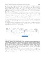
Fig. 1a shows one of the most widely used connection schemes of ac traction systems, where
the railroad substation is formed by a single-phase transformer feeding the traction load
from the utility power supply system. As the railroad substation is a single-phase load
which may lead to unbalanced utility supply voltages, several methods have been proposed
to reduce unbalance (Chen, 1994; Hill, 1994), such as feeding railroad substations at different
phases alternatively, and using special transformer connections (e.g. Scott-connection), SVCs
or external balancing equipment. To simplify the study of these methods, the single-phase
transformer is commonly considered ideal and the traction load is represented by its
equivalent inductive impedance, Z
L
= R
L
+ jX
L
, obtained from its power demand at the
fundamental frequency, Fig. 1b (Arendse & Atkinson-Hope, 2010; Barnes & Wong, 1991;
Chen, 1994; Mayer & Kropik, 2005; Qingzhu et al., 2010a, 2010b). According to Fig. 1c,
external balancing equipment consists in the delta connection of reactances (usually an
inductor Z
1
and a capacitor Z
2
) with the single-phase load representing the railroad
substation in order to load the network with balanced currents. This circuit, which is known
as Steinmetz circuit (ABB Power Transmission, n.d.; Barnes & Wong, 1991; Mayer & Kropik,

2005), is not the most common balancing method in traction systems but it is also used in
industrial high-power single-phase loads and electrothermal appliances (Chicco et al., 2009;
Chindris et. al., 2002; Mayer & Kropik, 2005).

(a)
Utility
supply
system
Railroad
substation
Traction
loa
d
A
B
C
X
L
Railroad
substation
Utility
supply
system
R
L
A
B
C
(b)
Z

2

Z
L
Steinmetz
circuit
Z
1
Railroad
substation
Traction
load
Utilit
y
supply
system
A
B
C
I
A
I
B
I
C
(c)

Fig. 1. Studied system: a) Railroad substation connection scheme. b) Simplified railroad
substation circuit. c) Steinmetz circuit.

Power Quality Harmonics Analysis and Real Measurements Data

174
R
1
R
L
I
A
I
B
I
C
A
X
2
X
1
X
L
Railroa d
substation
B
C
Utility
supply
system

Fig. 2. Detailed Steinmetz circuit.
Fig. 2 shows the Steinmetz circuit in detail. The inductor is represented with its associated

resistance, Z
1
= R
1
+ jX
1
, while the capacitor is considered ideal, Z
2
= − jX
2
. Steinmetz circuit
design aims to determine the reactances X
1
and X
2
to balance the currents consumed by the
railroad substation. Thus, the design value of the symmetrizing reactive elements is
obtained by forcing the current unbalance factor of the three-phase fundamental currents
consumed by the Steinmetz circuit (I
A
, I
B
, I
C
) to be zero. Balanced supply voltages and the
pure Steinmetz circuit inductor (i.e., R
1
= 0 ) are usually considered in Steinmetz circuit
design, and the values of the reactances can be obtained from the following approximated
expressions (Sainz et al., 2005):

() ()
1,apr 2,apr
22
33
(,) ; (,) ,
13 13
LL
LL LL
LL LL
RR
XR XR
λλ
λτ λτ
==
+−
(1)
where

2
1
,
L
L
L
LL
X
R
λ
τ

λ
−
== (2)
and
λ
L

= R
L
/|Z
L
| and |Z
L
| are the displacement power factor and the magnitude of the
single-phase load at fundamental frequency, respectively.
In (Mayer & Kropik, 2005), the resistance of the Steinmetz inductor is considered and the
symmetrizing reactance values are obtained by optimization methods. However, no
analytical expressions for the reactances are provided. In (Sainz & Riera, submitted for
publication), the following analytical expressions have recently been deduced

()
()
()
()()
{}
2
11 1
11 21
22
2

1
1
33
(,,) ; (,,) ,
13
13 3
L L
LL LL
LL
LL L
RR
XR XR
λτ τ
λτ λτ
λτ τ
λτττ
−−
==
+
−−+
(3)
where
τ
1
= R
1
/X
1
=
λ

1
/(1 –
λ
1
2
)
1/2
is the R/X ratio of the Steinmetz circuit inductor, and
λ
1
= R
1
/|Z
1
| and |Z
1
| are the displacement power factor and the magnitude of the
Steinmetz circuit inductor at the fundamental frequency, respectively. It must be noted that
(1) can be derived from (3) by imposing
τ
1
= 0 (and therefore
λ
1
/
τ
1
= 1). The Steinmetz
Characterization of Harmonic Resonances in
the Presence of the Steinmetz Circuit in Power Systems

175
circuit under study (with an inductor X
1
and a capacitor X
2
) turns out to be possible only
when X
1
and X
2
values are positive. Thus, according to (Sainz & Riera, submitted for
publication), X
1
is always positive while X
2
is only positive when the displacement power
factor of the single-phase load satisfies the condition

1
2
1
3
1,
21
LLC
τ
λλ
τ
+

≥≥ =
+
(4)
where the typical limit
λ
LC
= (√3)/2 can be obtained from (4) by imposing
τ
1
= 0 (Jordi et al.,
2002; Sainz & Riera, submitted for publication).
Supply voltage unbalance is considered in (Qingzhu et al., 2010a, 2010b) by applying
optimization techniques for Steinmetz circuit design, and in (Jordi et al., 2002; Sainz & Riera,
submitted for publication) by obtaining analytical expressions for the symmetrizing
reactances. However, the supply voltage balance hypothesis is not as critical as the pure
Steinmetz circuit inductor hypothesis. Harmonics are not considered in the literature in
Steinmetz circuit design and the reactances are determined from the fundamental waveform
component with the previous expressions. Nevertheless, Steinmetz circuit performance in
the presence of waveform distortion is analyzed in (Arendse & Atkinson-Hope, 2010; Chicco
et al., 2009). Several indicators defined in the framework of the symmetrical components are
proposed to explain the properties of the Steinmetz circuit under waveform distortion.
The introduction of thyristor-controlled reactive elements due to the recent development of
power electronics and the use of step variable capacitor banks allow varying the Steinmetz
circuit reactances in order to compensate for the usual single-phase load fluctuations,
(Barnes & Wong, 1991; Chindris et al., 2002). However, the previous design expressions
must be considered in current dynamic symmetrization and the power signals are then
treated by the controllers in accordance with the Steinmetz procedure for load balancing
(ABB Power Transmission, n.d.; Lee & Wu, 1993; Qingzhu et al., 2010a, 2010b).
3. Steinmetz circuit impact on power system harmonic response
The power system harmonic response in the presence of the Steinmetz circuit is analyzed from

Fig. 3. Two sources of harmonic disturbances can be present in this system: a three-phase non-
linear load injecting harmonic currents into the system or a harmonic-polluted utility supply
system. In the former, the parallel resonance may affect power quality because harmonic
voltages due to injected harmonic currents can be magnified. In the latter, series resonance
may affect power quality because consumed harmonic currents due to background voltage
distortion can also be magnified. Therefore, the system harmonic response depends on the
equivalent harmonic impedance or admittance “observed” from the three-phase load or the
utility supply system, respectively. This chapter, building on work developed in (Sainz et al.,
2007, in press), summarizes the above research on parallel and series resonance location and
unifies this study. It provides an expression unique to the location of the parallel and series
resonance considering the Steinmetz circuit inductor resistance.
In Fig. 3, the impedances
Z
Lk
= R
L
+ jkX
L
, Z
1k
= R
1
+ jkX
1
and Z
2k
= −jX
2
/k represent the
single-phase load, the inductor and the capacitor of the Steinmetz circuit at the fundamental

(
k = 1) and harmonic frequencies (k > 1). Note that impedances Z
L1
, Z
11
and Z
21
correspond
to impedances Z
L
, Z
1
and Z
2
in Section 2, respectively. Moreover, parameter d
C
is introduced
in the study representing the degree of the Steinmetz circuit capacitor degradation from its

Power Quality Harmonics Analysis and Real Measurements Data

176
design value [(1) or (3)]. Thus, the capacitor value considered in the harmonic study is d
C
·C,
i.e. −
j1/(d
C
·C·ω
1

·k) = −j·(X
2
/k)/d
C
= Z
2k
/d
C
where ω
1
= 2π·f
1
and f
1
is the fundamental
frequency of the supply voltage. This parameter allows examining the impact of the
capacitor bank degradation caused by damage in the capacitors or in their fuses on the
power system harmonic response. If
d
C
= 1, the capacitor has the design value [(1) or (3)]
whereas if
d
C
< 1, the capacitor value is lower than the design value.

R
1
R
L

(
X
2
/
k
)/
d
C
k·X
1
k·X
L
Utility
supply
system
Three-phase
load


Fig. 3. Power system harmonic analysis in the presence of the Steinmetz circuit.
3.1 Study of the parallel resonance
This Section examines the harmonic response of the system “observed” from the three-phase
load. It implies analyzing the passive set formed by the utility supply system and the
Steinmetz circuit (see Fig. 4). The system harmonic behavior is characterized by the
equivalent harmonic impedance matrix,
Z
Busk
, which relates the k
th
harmonic three-phase

voltages and currents at the three-phase load node, V
k
= [V
Ak
V
Bk
V
Ck
]
T
and I
k
= [I
Ak
I
Bk
I
Ck
]
T
.
Thus, considering point N in Fig. 4 as the reference bus, this behavior can be characterized
by the voltage node method,

C
Z
Bus
k
I
Ak

N
R
S
k·X
S
I
Bk
I
Ck
B
A
V
Ck
V
Bk
V
Ak
R
1
R
L
(
X
2
/
k
)/
d
C
k·X

1
k·X
L

Fig. 4. Study of the parallel resonance in the presence of the Steinmetz circuit.
Characterization of Harmonic Resonances in
the Presence of the Steinmetz Circuit in Power Systems

177

1
12 1 2
11
22
,
AAk ABk ACk Ak
Ak
k k k BAk BBk BCk Bk
Bk
CAk CBk CCk Ck
Ck
Sk k k k k AkCC
kSkkLk Lk Bk
kLkSkkLkCkCC
VZZZI
VZZZI
VZZZI
YYdY Y dY I
YYYY Y I
dY Y Y dY Y I

−
 
 
=⋅ =⋅
 
 
 
++ − −




=− ++ − ⋅




−−++


Bus
VZ I
(5)
where
•
Y
Sk
= Z
Sk
–1

= (R
S
+jkX
S
)
–1
corresponds to the admittance of the power supply system,
which includes the impedance of the power supply network, the short-circuit
impedance of the three-phase transformer and the impedance of the overhead lines
feeding the Steinmetz circuit and the three-phase linear load.
•
Y
Lk
, Y
1k
and d
C
·Y
2k
correspond to the admittances of the Steinmetz circuit components
(i.e., the inverse of the impedances Z
Lk
, Z
1k
and Z
2k
/d
C
in Section 3, respectively).
It can be observed that the diagonal and non-diagonal impedances of the harmonic

impedance matrix
Z
Busk
(i.e., Z
AAk
to Z
CCk
) directly characterize the system harmonic
behavior. Diagonal impedances are known as phase driving point impedances (Task force
on Harmonic Modeling and Simulation, 1996) since they allow determining the contribution
of the harmonic currents injected into any phase
F (I
Fk
) to the harmonic voltage of this phase
(V
Fk
). Non–diagonal impedances are the equivalent impedances between a phase and the
rest of the phases since they allow determining the contribution of the harmonic currents
injected into any phase
F (I
Fk
) to the harmonic voltage of any other phase G (V
Gk
, with G ≠ F).
Thus, the calculation of both sets of impedances is necessary because a resonance in either of
them could cause a high level of distortion in the corresponding voltages and damage
harmonic power quality.
As an example, a network as that in Fig. 4 was constructed in the laboratory and its
harmonic response (i.e.,
Z

Busk
matrix) was measured with the following per unit data
(U
B
= 100 V and S
B
= 500 VA) and considering two cases (d
C
= 1 and 0.5):
•
Supply system: Z
S1
= 0.022 +j0.049 pu.
• Railroad substation: R
L
= 1.341 pu,
λ
L
= 1.0.
•
External balancing equipment: According to (1) and (3), two pairs of reactances were
connected with the railroad substation, namely
X
1, apr
= 2.323 pu and X
2, apr
= 2.323 pu
and
X
1

= 2.234 pu and X
2
= 2.503 pu. The former was calculated by neglecting the
inductor resistance (1) and the latter was calculated by considering the actual value of
this resistance (3) (
R
1
≈ 0.1342 pu, and therefore
τ
1
≈ 0.1341/2.234 = 0.06).
Considering that the system fundamental frequency is 50 Hz, the measurements of the
Z
Busk

impedance magnitudes (i.e., |Z
AAk
| to |Z
CCk
|) with X
1, apr
and X
2, apr
are plotted in Fig. 5 for
both cases (d
C
= 1 in solid lines and d
C
= 0.5 in broken lines). It can be noticed that
•

The connection of the Steinmetz circuit causes a parallel resonance in the
Z
Busk
impedances that occurs in phases A and C, between which the capacitor is
connected, and is located nearly at the same harmonic for all the impedances (labeled as
k
p, meas
). This asymmetrical resonant behavior has an asymmetrical effect on the
harmonic voltages (i.e., phases
A and C have the highest harmonic impedance, and
therefore the highest harmonic voltages.)

Power Quality Harmonics Analysis and Real Measurements Data

178
|Z
AB
|
≈
|Z
BA
| (pu)|Z
AC
|
≈
|Z
CA
| (pu)|Z
BC
|

≈
|Z
CB
| (pu)
1.5
1.0
0.5
0
|Z
AA
| (pu)
1.5
1.0
0.5
0
|Z
BB
| (pu)
1.5
1.0
0.5
0
|Z
CC
| (pu)
1
k
3579111
k
357911

k
p
, meas

≈
5.02
k
p, meas
≈ 7.2

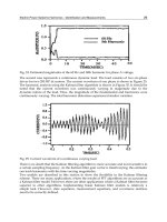
Fig. 5. Measured impedance - frequency matrix in the presence of the Steinmetz circuit with
X
1, apr
= X
2, apr
= 2.323 pu (solid line: d
C
= 1; broken line: d
C
= 0.5).
•
In the case of d
C
= 1 (in solid lines), the connection of the Steinmetz circuit causes a
parallel resonance measured close to the fifth harmonic (
k
p, meas
≈ 251/50 = 5.02, where
251 Hz is the frequency of the measured parallel resonance.)
•

If the Steinmetz circuit suffers capacitor bank degradation, the parallel resonance is
shifted to higher frequencies. In the example, a 50% capacitor loss (i.e.,
d
C
= 0.5 in
broken lines) shifts the parallel resonance close to the seventh harmonic
(
k
s, meas
≈ 360/50 = 7.2, where 360 Hz is the frequency of the measured parallel
resonance.)
The measurements of the
Z
Busk
impedance magnitudes (i.e. |Z
AAk
| to |Z
CCk
|) with X
1
and
X
2
are not plotted for space reasons. In this case, the parallel resonance shifts to k
p, meas
≈ 5.22
(
d
C
= 1) and k

p, meas
≈ 7.43 (d
C
= 0.5) but the general conclusions of the X
1, apr
and X
2, apr
case
are true.
Characterization of Harmonic Resonances in
the Presence of the Steinmetz Circuit in Power Systems

179
C
Y
Bus
k
I
A
k
N
R
1
R
L
(
X
2
/
k

)/
d
C
k·X
1
k·X
L
R
S
k·X
S
I
Bk
I
Ck
B
A
V
Ck
V
Bk
V
A
k
Z
pk
I II

Fig. 6. Study of the series resonance in the presence of the Steinmetz circuit.
3.2 Study of the series resonance

This Section studies the harmonic response of the system “observed” from the utility supply
system. It implies analyzing the passive set formed by the supply system impedances, the
Steinmetz circuit and the three-phase load (see Fig. 6). The system harmonic behavior is
characterized by the equivalent harmonic admittance matrix,
Y
Busk
, which relates the k
th

harmonic three-phase currents and voltages at the node I, I
I
k
= [I
Ak
I
Bk
I
Ck
]
T
and
V
I
k
= [V
Ak
V
Bk
V
Ck

]
T
, respectively. Thus, considering point N in Fig. 6 as the reference bus,
this behavior can be characterized by the voltage node method,

II-II I
I
II-I II II
11 2
12
23
00 0 0
000 0
00 0 0
000
00 0
000
kk k
k
kk k
Ak Sk Sk
Bk Sk Sk
Ck Sk Sk
Sk T k k kC
Sk k T k Lk
Sk k Lk T k
C
IY Y
IY Y
IY Y

YYYdY
YYYY
YdYYY



=⋅





−
 
 
−
 
 
−
 =
 
−−−
 
 
−− −
 
−− −

 
YY V

I
0
YYV
II
II
II
,
Ak
Bk
Ck
Ak
Bk
Ck
V
V
V
V
V
V










⋅












(6)
and

()
1
I I I-II II II-I I I
,
Ak AAk ABk ACk
Ak
k Bk k k k k k k k BAk BBk BCk
Bk
Ck CAk CBk CCk
Ck
IYYYV
IYYYV
IYYYV
−
   
   

==− = = ⋅
   
   
   
Bus
IYYYYVYV
(7)
where

11221
32
;
.
T k Sk Pk k k T k Sk Pk k Lk
C
T k Sk Pk Lk kC
Y YYYdY Y YYYY
YYYYdY
=+++ =+++
=+++
(8)
Admittances Y
Sk
, Y
Lk
, Y
1k
and d
C
·Y

2k
were already introduced in the parallel resonance
location and Y
Pk
= Z
Pk
–1
= g
LM#
(|Z
P1
|,
λ
P
, k) is the three-phase load admittance. The function
g
LM#
(·) represents the admittance expressions of the load models 1 to 7 proposed in (Task

Power Quality Harmonics Analysis and Real Measurements Data

180
force on Harmonic Modeling and Simulation, 2003), and |Z
P1
| and
λ
P
are the magnitude
and the displacement power factor of the load impedances at the fundamental frequency,
respectively. For example, the expression g

LM1
(|Z
P1
|,
λ
P
, k) = 1/{|Z
P1
|·(
λ
P
+ jk(1 –
λ
P
2
)
1/2
)}
corresponds to the series R-L impedance model, i.e. the model LM1 in (Task force on
Harmonic Modeling and Simulation, 2003).
It can be observed that the diagonal and non-diagonal admittances of the harmonic
admittance matrix
Y
Busk
(i.e., Y
AAk
to Y
CCk
) directly characterize system harmonic behavior.
Diagonal admittances allow determining the contribution of the harmonic voltages at any

phase F (V
Fk
) to the harmonic currents consumed at this phase (I
Fk
). Non–diagonal
admittances allow determining the contribution of the harmonic voltages at any phase F
(V
Fk
) to the harmonic currents consumed at any other phase G (I
Gk
, with G ≠ F). Thus, the
calculation of both sets of admittances is necessary because this resonance could lead to a
high value of the admittance magnitude, magnify the harmonic currents consumed in the
presence of background voltage distortion and damage harmonic power quality.
As an example, a network as that in Fig. 6 was constructed in the laboratory and its
harmonic response (i.e.,
Y
Busk
matrix) was measured with the following per unit data
(U
B
= 100 V and S
B
= 500 VA) and considering two cases (d
C
= 1 and 0.5):
•
Supply system: Z
S1
= 0.076 +j0.154 pu.

• Railroad substation: R
L
= 1.464 pu, λ
L
= 0.95.
•
External balancing equipment: According to (1) and (3), two pairs of reactances were
connected with the railroad substation, namely X
1, apr
= 1.790 pu and X
2, apr
= 6.523 pu
and X
1
= 1.698 pu and X
2
= 10.03 pu. The former was calculated by neglecting the
inductor resistance (1) and the latter was calculated by considering the actual value of
this resistance (3) (R
1
≈ 0.1342 pu, and therefore
τ
1
≈ 0.1341/1.698 = 0.079).
•
Three-phase load: Grounded wye series R-L impedances with |Z
P1
| = 30.788 pu and
λ
P

= 0.95 are connected, i.e. the three-phase load model LM1 in (Task force on Harmonic
Modeling and Simulation, 2003).
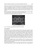
Considering that the system fundamental frequency is 50 Hz, the measurements of the
Y
Busk

admittance magnitudes (i.e. |Y
AAk
| to |Y
CCk
|) with X
1, apr
and X
2, apr
are plotted in Fig. 7 for
both cases (d
C
= 1 in solid lines and d
C
= 0.5 in broken lines). It can be noted that
•
The connection of the Steinmetz circuit causes a series resonance in the
Y
Busk
admittances that occurs in phases A and C, between which the capacitor is
connected, and is located nearly at the same harmonic for all the admittances (labeled as
k
s, meas
). This asymmetrical resonant behavior has an asymmetrical effect on the
harmonic consumed currents (i.e., phases A and C have the highest harmonic

admittance, and therefore the highest harmonic consumed currents.)
•
In the case of d
C
= 1 (in solid lines), the connection of the Steinmetz circuit causes a
series resonance measured close to the fifth harmonic (k
s, meas
≈ 255/50 = 5.1, where
255 Hz is the frequency of the measured series resonance.)
• If the Steinmetz circuit suffers capacitor bank degradation, the series resonance is
shifted to higher frequencies. In the example, a 50% capacitor loss (i.e., d
C
= 0.5 in
broken lines) shifts the series resonance close to the seventh harmonic
(k
s, meas
≈ 365/50 = 7.3, where 365 Hz is the frequency of the measured series resonance.)
The measurements of the
Y
Busk
admittance magnitudes (i.e., |Y
AAk
| to |Y
CCk
|) with X
1
and X
2

are not plotted for space reasons. In this case, the series resonance shifts to k

s, meas
≈ 6.31 (d
C
= 1)
and k
s, meas
≈ 8.83 (d
C
= 0.5) but the general conclusions of the X
1, apr
and X
2, apr
case are true.
Characterization of Harmonic Resonances in
the Presence of the Steinmetz Circuit in Power Systems

181


|
Y
ABk
|
≈
|
Y
BAk
| (pu)|
Y
ACk

|
≈
|
Y
CAk
| (pu)|
Y
BCk
|
≈
|
Y
CBk
| (pu)
1
k
3579
k
s, meas
≈ 7.3
k
s,
meas
≈ 5.1
1
k
3579
|
Y
AAk

| (pu)
2.5
1.0
0.5
0
1.5
2.0
|
Y
BBk
| (pu)
2.5
1.0
0.5
0
1.5
2.0
|
Y
CCk
| (pu)
2.5
1.0
0.5
0
1.5
2.0


Fig. 7. Measured admittance - frequency matrix in the presence of the Steinmetz circuit with

X
1, apr
= 1.790 pu and X
2, apr
= 6.523 pu (solid line: d
C
= 1; broken line: d
C
= 0.5).
4. Analytical study of power system harmonic response
In this Section, the magnitudes of the most critical Z
Busk
impedances (i.e., |Z
AAk
|, |Z
CCk
|,
|Z
ACk
| and |Z
CAk
|) and Y
Busk
admittances (i.e., |Y
AAk
|, |Y
CCk
|, |Y
ACk
| and |Y

CAk
|) are
analytically studied in order to locate the parallel and series resonance, respectively.
4.1 Power system harmonic characterization
The most critical Z
Busk
impedances are obtained from (5):

Power Quality Harmonics Analysis and Real Measurements Data

182

22
12 112
22
() ()
;
,
Sk Sk Stz k Lk Stz k Sk Sk Stz k k Stz k
AAk CCk
Sk k Sk k
Stz k k Sk
C
ACk CAk
Sk k
YYY Y Y YYY Y Y
ZZ
YD YD
YdYY
ZZ

YD
+++ +++
==
+
==
(9)
where

=+ + = + +
=+ +⋅
11 2 2 1 212
2
12
;
23.
Stz k k k Lk Stz k Lk k Lk k k k
CCC
k Sk Sk Stz k Stz k
Y Y dY Y Y Y Y Y dY Y dY
DY YY Y
(10)
The harmonic of the parallel resonance numerically obtained as the maximum value of the
above impedance magnitudes is located nearly at the same harmonic for all the impedances
(Sainz et al., 2007) and labeled as k
p, n
.
The most critical
Y
Busk
admittances are obtained from (7):

++
==
+⋅ +⋅
++
==
+⋅
() ()
() ()
2
22 2
()
() ()
;
()
,
PP
Sk Sk Pk Sk Sk Pk
AAk AAk CCk CCk
AAk CCk
PP
Sk k Pk k Sk k Pk k
Sk Sk k Stz k Pk kCC
ACk CAk
P
Sk k Pk k
YYN YN YYN YN
YY
YD Y D YD Y D
Y Y dY Y Y dY

YY
YD Y D
(11)
where

=++⋅ =++⋅
=+⋅ + +⋅ + + + +⋅
=+⋅ + +⋅ + + + +⋅
12 2 2 2
() 2
1212
() 2
12 2 1
()2; ()2
2( )3( ( ))(2)
2( )3( ( ))(2)
Sk k k Stz k Sk Lk k Stz kCC
AAk CCk
P
Pk Sk Stz k Pk Stz k Sk k k Sk Sk LkC
AAk
P
Pk Sk Stz k Pk Stz k Sk Lk k Sk Sk k
C
CCk
NYYdY Y NYYdY Y
N Y Y Y Y Y YY dY YY Y
N Y Y Y Y Y YY dY YY Y
D
=+ +⋅ +⋅ + +

() 2 2
121
(3 2 ) 3 ( ) 4 .
P
k Pk Sk Stz k Pk Sk Stz k Sk Stz k
YY YY YY YY
(12)
The harmonic of the series resonance numerically obtained as the maximum value of the
above admittance magnitudes is located nearly at the same harmonic for all the admittances
(Sainz et al., in press) and labeled as k
s, n
.
Since the expressions of the
Y
Busk
admittances (11) are too complicated to be analytically
analyzed, the admittance Y
Pk
is not considered in their determination (i.e., Y
Pk
= 0), and they
are approximated to

≈= ≈=
+
=≈==
,apx ,apx
22
, apx ,apx
;

()
.
Sk Sk
A
Ak CCk
AAk AAk CCk CCk
kk
Sk Sk k Stz kC
ACk CAk ACk ACk
k
YN YN
YY YY
DD
YYdY Y
YYY Y
D
(13)
This approximation is based on the fact that, the three-phase load does not influence the
series resonance significantly if large enough, (Sainz et al., 2009b). The harmonic of the
series resonance numerically obtained as the maximum value of the above admittance
magnitudes is located nearly at the same harmonic for all the admittances (Sainz et al., in
press) and labeled as k
s, napx
.
Characterization of Harmonic Resonances in
the Presence of the Steinmetz Circuit in Power Systems

183
It must be noted that (9) and (13) depend on the supply system and the Steinmetz circuit
admittances (i.e., Y

Sk
, Y
Lk
, Y
1k
and d
C
·Y
2k
) and (11) depends on the previous admittances and
three-phase load admittances (i.e., Y
Sk
, Y
Lk
, Y
1k
, d
C
·Y
2k
and Y
Pk
). In the study, these
admittances are written as

()
()
()()
{}
()

()
2
1
1
11
1
2
1
2 1LM #
2
1
11 1113
;;
1
3
13 3
;,,,
3
LL
Sk Lk k
SLL
L
CL L L
C
k Pk PC P
L
Yj Y Y j
kX R jk jk X k
R
d

d
dY jk Y g Z k
jX k
R
λτ τ
τλ
τ
λτττ
λ
τ

+
≈− = ≈ =−

+⋅
−

−−+
== =
−
−
(14)
where (3) is used to obtain the Steinmetz circuit components X
1
and X
2
, and g
LM#
(·)
represents the three-phase load admittance models 1 to 7 proposed in (Task force on

Harmonic Modeling and Simulation, 2003). Thus, it is observed that the
Z
Busk
impedances
and Y
Busk
admittances are functions of eight variables, namely
• the harmonic order k,
•
the supply system fundamental reactance X
S
,
•
the single-phase load resistance R
L
,
•
the parameter
τ
L
, i.e. the single-phase load fundamental displacement power factor
λ
L

(2),
•
the R/X ratio of the Steinmetz circuit inductor
τ
1
,

•
the degradation parameter d
C
,
•
the magnitude of the linear load fundamental impedance |Z
P1
| and
• the linear load fundamental displacement power factor
λ
P
.
It is worth pointing out that the resistance of the supply system is neglected (i.e.,
Z
Sk
= R
S
+ jkX
S
≈ jkX
S
) and the resistance of the Steinmetz circuit is only considered in the
inductor design [i.e., Z
1k
= R
1
+ jkX
1
≈ jkX
1

and Z
2k
= −j·X
2
/k, with X
1
and X
2
obtained from
(3)]. This is because the real part of these impedances does not modify the series resonance
frequency significantly (Sainz et al., 2007, 2009a) while the impact of R
1
on Steinmetz circuit
design modifies the resonance. This influence is not considered in the previous harmonic
response studies.
In order to reduce the above number of variables, the
Z
Busk
impedances and Y
Busk

admittances are normalized with respect to the supply system fundamental reactance X
S
.
For example, the normalized magnitudes |Z
AAk
|
N
and |Y
AAk

|
N
can be expressed from (9)
and (11) as

{
}
{}
2
2
12
2
N
()
3
NN
()
3
()
1
,
()
,
Sk Sk Stz k Lk Stz k
S
AAk
AAk
Sk k
SS S
P

Sk Sk PkS
AAk AAk
AAk AAkSS
P
Sk k Pk k
S
XY Y Y Y Y
Z
Z
XX XYD
XY Y N Y N
YXYX
XYD Y D
+++
==
+
==
+⋅
(15)
where (15) has only terms X
S
·Y
Sk
, X
S
·Y
Lk
, X
S
·Y

1k
, X
S
·d
C
·Y
2k
and X
S
·Y
Pk
, which can be
rewritten from (14) as

Power Quality Harmonics Analysis and Real Measurements Data

184

()
()
()
()()
{}
()
LM #, N
2
1
1
11 1
1

2
1
2
22
1
11
,,,,
1
11 13
,
3
13 3
,
3
Sk Lk PkSS SPP
LL
SLL
kS
L
CL L L
SC C
k
SC
L
XY j XY XY g z k
krjk
X
XY j j
jk X k x k
r

d
Xd d
XdY jk jk
jX k x
r
λ
τ
λτ τ
λ
τ
λτττ
τ
=− = =
+

+
==−=−

⋅⋅
−

−−+
===
−
−
(16)
where g
LM#, N
(·) represents the normalized expressions of the three-phase load models 1 to 7
proposed in (Task force on Harmonic Modeling and Simulation, 2003), r

L
= R
L
/X
S
and
z
P
= |Z
P1
|

/X
S
. The normalized expressions g
LM#, N
(·) are obtained and presented in (Sainz
et al., 2009a) but are not included in the present text for space reasons. As an example, the
normalized expression of model LM1 in (Task force on Harmonic Modeling and Simulation,
2003) is g
LM1, N
(z
p
,
λ
P
, k) = 1/{z
p
·(
λ

P
+ jk(1−
λ
P
2
)
1/2
)} (Sainz et al., 2009a).
From (15), it is interesting to note that the normalization does not modify the parallel and
series resonance (k
p, n
, k
s, n
and k
s, napx
), but the number of variables of the normalized Z
Busk

impedances and Y
Busk
admittances are reduced to seven (16), i.e.,
• the harmonic order k,
•
the ratio of the single-phase load resistance to the supply system fundamental reactance
r
L
= R
L
/X
S

,
•
the parameter
τ
L
, i.e. the single-phase load fundamental displacement power factor
λ
L

(2),
•
the R/X ratio of the Steinmetz circuit inductor
τ
1
,
•
the degradation parameter d
C
,
•
the ratio of the linear load fundamental impedance magnitude to the supply system
fundamental reactance z
P
= |Z
P1
|

/X
S
and

• the linear load fundamental displacement power factor
λ
P
.
Moreover, the usual ranges of values of these variables can be obtained by relating them
with known parameters to study resonances under power system operating conditions.
Thus, the power system harmonic response is analyzed for the following variable ranges:
•
Harmonic: k = (1, , 15).
•
Single-phase load: r
L
= (5, , 1000) and
λ
L
= (0.9, , 1).
•
Steinmetz circuit inductor:
τ
1
= (0, , 0.5).
•
Degradation parameter: d
C
= (0.25, , 1).
•
Linear load: z
P
= (5, , 1000) and
λ

P
= (0.9, , 1).
The ratios r
L
and z
P
are equal to the ratios
λ
L
·S
S
/S
L
and S
S
/S
P
(Sainz et al., 2009a), where S
S

is the short-circuit power at the PCC bus, S
L
is the apparent power of the single-phase load
and S
P
is the apparent power of the three-phase load. Thus, the range of these ratios is
determined considering the usual values of the ratios S
S
/S
L

and S
S
/S
P
(Chen, 1994; Chen &
Kuo, 1995) and the fundamental displacement power factors
λ
L
and
λ
P
.
In next Section, the normalized magnitudes of the most critical
Z
Busk
impedances (9) and
approximated Y
Busk
admittances (13) are analytically studied to obtain simple expressions
for locating the parallel and series resonance. Thus, these expressions are functions of the
following five variables only: k, r
L
= R
L
/X
S
,
λ
L
,

τ
1
and d
C
.
Characterization of Harmonic Resonances in
the Presence of the Steinmetz Circuit in Power Systems

185
The series resonance study in the next Section is only valid for z
P
> 20 because the
approximation of not considering the three-phase load admittance (i.e., Y
Pk
= 0 ) is based on
the fact that this load does not strongly influence the series resonance if z
P
is above 20.
Nevertheless, the magnitude of the normalized admittances at the resonance point is low for
z
P
< 20 and the consumed currents do not increase significantly (Sainz et al., 2009a).
4.2 Analytical location of the parallel and series resonance
It is numerically verified that the parallel and series resonance, i.e. the maximum magnitude
values of the normalized
Z
Busk
impedances and approximated Y
Busk
admittances [obtained

from (9) and (13)] with respect to the harmonic k respectively, coincide with the minimum
value of their denominators for the whole range of system variables. Thus, from (9) and (13),
these denominators can be written as

()()()
() () ()
,apx ,apx ,apx
NN N
NN N
22
12 34
Den Den Den
Den Den Den
()(),
AAk CCk ACk
AAk CCk ACk
YYkY
kZ kZ kZ
kkHk H j Hk H
==⋅
=⋅ =⋅ =⋅
=++⋅+
(17)
where

2
1112 1
2
31 4 1
(2 3) 3 ; ( ( 2) 2 3)

(2 3) ; ( 2)
LL LL LL
C
LL
C
x
Hr x x H xr r
d
x
Hrx H rx
d
τττ

=++ =− +++



=+ =− +


(18)
and

() ()
()()
{}
2
11
1
12

2
1
1
33
;.
13
13 3
LL
L
L
LL L
rr
xx
ττ
λ
λτ
τ
λτττ
−−

==

+
−−+

(19)
From (17), it is observed that the series resonances of |Y
AAk, apx
|
N

and |Y
CCk, apx
|
N

admittances match up because their denominators are the same. This is true for the series
resonance of |Y
ACk, apx
|
N
admittance and the parallel resonance of |Z
AAk
|
N
, |Z
CCk
|
N
and
|Z
ACk
|
N
impedances. However, despite the discrepancy in the denominator degrees, it is
numerically verified that the harmonic of the parallel and series resonance is roughly the
same for all the impedances and admittances. Then, these resonances are located from the
minimum value of the |Y
ACk, apx
|
N

,

|Z
AAk
|
N
, |Z
CCk
|
N
and |Z
ACk
|
N
denominator because it is
the simplest. In the study, this denominator is labeled as |Δ
k
| for clarity and the harmonic
of the parallel and series resonance numerically obtained as the minimum value of |Δ
k
| is
labeled as k
r,
Δ
for both resonances. This value is analytically located by equating to zero the
derivative of |Δ
k
|
2
with respect to k, which can be arranged in the following form:

()
2
42 4 2
112 ,a1,a2
6( ) 0,
k
rr
HkkGkG k Gk G
k
∂Δ
=++ ++=
∂
(20)

Power Quality Harmonics Analysis and Real Measurements Data

186
where k
r, a
is the harmonic of the parallel and series resonance analytically obtained and

22
21 3 2 43
12
22
11
2(2 ) 2
;.
33

HH H H HH
GG
HH
⋅+ +⋅
==
⋅⋅
(21)
Thus, the root of equation (20) allows locating the parallel and series resonance:

2
11 2
,a
4
.
2
r
GG G
k
−+ −⋅
= (22)

(a)
(b)
|Z
AAk
|
N
(pu)
35
0

17.5
|Y
AAk
|
N
, |Y
AAk
, apx
|
N
(pu)
0.8
0.4
0
4
k
567 98
5
0
2.5
|Δ
k
|/10
4
(pu)
1
0
0.5
|Δ
k

|/10
4
(pu)
4
k
567 98
k
p, n
= k
r,
Δ
= 4.94
k
p, n
= 7.04
k
r,
Δ
= 7.05
d
C
=0.5
τ
1
=0%
d
C
= 1.0
k
p, n

= 5.13
k
p, n
= k
r,
Δ
= 7.33
τ
1
=6.0%
k
r,
Δ
= 5.14
k
s, n
= 5.00
k
r,
Δ
= 4.95
k
s, napx
= 4.97
k
s, n
= 7.09
k
r,
Δ

= 7.03
k
s, napx
= 7.04
k
s, n
= 6.22
k
r,
Δ
= 6.16
k
s, napx
= 6.18
k
s, n
= 8.81
k
r,
Δ
= 8.74
k
s, napx
= 8.75
τ
1
=7.9%
τ
1
=0%

d
C
= 0.5d
C
= 1.0

Fig. 8. Resonance location: a) Parallel resonance (power system data in Section 3.1:
X
S
= 0.049 pu, R
L
= 1.341 pu and
λ
L
= 1.0). b) Series resonance (power system data in
Section 3.2: X
S
= 0.154 pu, R
L
= 1.464 pu,
λ
L
= 0.95, |Z
P1
| = 30.788 pu,
λ
P
= 0.95 and three-
phase load model LM1).
To illustrate the above study, Fig. 8 shows |Z

AAk
|
N
, |Y
AAk
|
N
, |Y
AAk, apx
|
N
and |Δ
k
| for the
power systems presented in the laboratory tests of Sections 3.1 and 3.2, and the analytical
results of the resonances (22) for these systems are
•
Parallel resonance: k
r, a
= 4.94 and 7.05 (
τ
1
= 0 and d
C
= 1.0 and 0.5, respectively) and
k
r, a
= 5.13 and 7.33 (
τ
1

= 6.0% and d
C
= 1.0 and 0.5, respectively).
Characterization of Harmonic Resonances in
the Presence of the Steinmetz Circuit in Power Systems

187
• Series resonance: k
r, a
= 4.95 and 7.03 (
τ
1
= 0 and d
C
= 1.0 and 0.5, respectively) and
k
r, a
= 6.16 and 8.74 (
τ
1
= 7.9% and d
C
= 1.0 and 0.5, respectively).
From these results, it is seen that
•
As the variable z
P
= 30.788/0.154 = 199.9 > 20, the numerical results obtained from
|Y
AAk, apx

|
N
are similar to those obtained from |Y
AAk
|
N
, and k
s, n
≈ k
s, napx
.
• The harmonic of the |Z
AAk
|
N
and |Y
AAk, apx
|
N
(and therefore |Y
AAk
|
N
) maximum values
nearly coincides with the harmonic of the |Δ
k
| minimum value, k
r,
Δ
≈ k

p, n
and
k
r,
Δ
≈ k
s, napx
, and that (22) provides the harmonic of the parallel and series resonance
correctly, i.e. k
r, a
≈ k
p, n
and k
r, a
≈ k
s, napx
.
•
Although the resistances R
S
and R
1
of the supply system and the Steinmetz circuit
inductor are neglected in the analytical study [i.e., Z
Sk
≈ j·k·X
S
and Z
1k
≈ j·k·X

1
in (14)],
the results are in good agreement with the experimental measurements in Sections 3.1
and 3.2, i.e. k
r, a
≈ k
p, meas
and k
r, a
≈ k
s, meas
. However, the magnitude values obtained
numerically are greater than the experimental measurements (e.g.,
|Z
AAk
| = X
S
·|Z
AAk
|
N
= 0.049·33.03 = 1.62 pu for k
p, n
= 7.04 in the
τ
1
= 0% and d
C
= 0.5
plot of Fig. 8 and |Z

AAk
| ≈ 1.1 pu for k
p, meas
= 7.2 in Fig. 5 or
|Y
AAk
| = |Y
AAk
|
N
/X
S
= 0.73/0.154 = 4.74 pu for k
s, n
= 7.09 in the
τ
1
= 0% and d
C
= 0.5
plot of Fig. 8 and |Y
AAk
| ≈ 2.1 pu for k
p, meas
= 7.2 in Fig. 7).
• The influence of the resistance R
1
on Steinmetz circuit design (3) shifts the parallel and
series resonance to higher frequencies. This was also experimentally verified in the
laboratory test of Section 3.

Fig. 9 compares k
r, a
, with k
p, n
and k
s, n
. Considering the validity range of the involved
variables, the values leading to the largest differences are used. It can be observed that k
r, a

provides the correct harmonic of the parallel and series resonance. The largest differences
obtained are below 10% and correspond to k
s, n
when z
P
= 20, which is the lowest acceptable
z
P
value to apply the k
r, a
analytical expression. Although only the linear load model LM1 is
considered in the calculations, it is verified that the above conclusions are true for the other
three-phase load models.

k
p
, n
, k
s
, n

, k
r
, a
45
25
5
35
15
10
0
|k
res

−
k
r
, a
|/k
res
(%)
2
4
6
8
5
r
L
50 100 150 300200 250
λ
L

=1.0,
d
C
=0.5,
τ
1
=0.4
k
r, a
k
s, n
(z
P
= 20,
λ
P
= 0.95, LM1)
k
s, n
(z
P
= 50,
λ
P
= 0.95, LM1)
k
p, n
, k
s, n
(z

P
=
∞
)

Fig. 9. Comparison between k
res
and k
r, a
(k
res
= k
p, n
or k
s, n
).
The previous research unifies the study of the parallel and series resonance, providing an
expression unique to their location. This expression is the same as in the series resonance
case (Sainz et al., 2007), but substantially improves those obtained in the parallel resonance
case (Sainz et al., in press). Moreover, the Steinmetz circuit inductor resistance is considered

Power Quality Harmonics Analysis and Real Measurements Data

188
in the analytical location of the resonances, making a contribution to previous studies. This
resistance, as well as damping the impedance values, shifts the resonance frequencies
because it influences Steinmetz circuit design (i.e., the determination of the Steinmetz circuit
reactances).
5. Sensitivity analysis of power system harmonic response
A sensitivity analysis of all variables involved in location of the parallel and series resonance

is performed from (22). Thus, considering the range of the variables, Fig. 10 shows the
contour plots of the harmonics where the parallel and series resonance is located. These
harmonics are calculated from the expression of k
r, a
, (22), and the
τ
1
range is fixed from (4)
considering the
λ
L
value. From Fig. 10, it can be noted that

τ
1
=0
τ
1
=0.2
τ
1
=0.4
d
C
(%)
100
50
25
75
3

5
7
9
11
13
15
17
r
L
(pu)

5 40 10020 60 80 100
r
L
(pu)

54020 60 80
r
L
(pu)

540 10020 60 80
τ
1
=0
τ
1
=0.1
τ
1

=0.2
τ
1
=0
τ
1
= 0.025
τ
1
=0.05
9
11
13 15 17 21 23
25
27
29
…
3
5
7
9
11
13
15
17
19
5
7
9
11

13
15
17
19
.
.
.
7
9
11
13
15
17
19
.
.
.
9
31
13
41
17
21 25
27
29
51
100
50
25
75

d
C
(%)
100
50
25
d
C
(%)
21
31
41
51
61
71
λ
L
= 0.9
33 43 53
63
73
83
93
…
λ
L
= 0.95
5
7
9

11
13
15
17
19
.
.
.
λ
L
= 1.0

Fig. 10. Contour plots of k
r, a
.