Multiprocessor Scheduling Part 12 pot

Multiprocessor Scheduling: Theory and Applications
320
LOAD/ UNLOAD PROCESS:
Parameter Value
Loading / unloading parts to/from pallets 0.3 min.
Moving pallets to load / unload storage buffers 0.2 min.
MATERIAL HANDLING SYSTEM:
Parameter Value
Number of AGVs 1
Transfer time between the stations 1.5 min.
OPERATORS:
Parameter Value
Number of operators 8
Operator transfer time between workstations 0.5 min
For each product type, Tables 1 and 2 show the operational sequences with required
resources and processing times without setup times.
Operations Machine required - Processing time
O-l M-l (4.5 min.) / M-3 (3.2 min.)
O-2 M-2 (4.5 min.) / M-4 (3.2 min.)
O-3 M-5 (9 min.) / M-6 (5.2 min.) / M-7 (6 min.) / M-3 (3.6 min.)
O-4 M-8 (2 min.)
O-5 M-9(1.5min.)
Table 1. Process plan of product type 1 (P
1
)
Operations Machine required - Processing time
O-l M-3 (3.7 min)
O-2 M-4 (5.3 min.)
O-3 M-5 (13 min.) / M-6 (7.5 min. for P
2
; 8.5 min. for P

3
) / M-3 (5.25 min.)
O-4 M-8 (2 min.)
O-5 M-9(1.5min.)
Table 2. Process plan of product type 2 and 3 (P
2
and P
3
)
Ten independent replications for each dispatching strategies were run for 180.000 operating
minutes (125 days with three 8 hr shifts) during the simulation of the PN model. In each run,
the shop is continuously loaded with job-orders that are numbered on arrival, and each run
produced one observation for each performance measure. Different random number seeds
were used to prevent correlation between the parallel runs of the factorial experiment. In
A Heuristic Rule-Based Approach for Dynamic Scheduling of Flexible Manufacturing Systems
321
order to ascertain when the system reaches a steady state, the shop parameters, such as
mean flow time of jobs and utilization level of machines, were observed, and it has been
found that the system became stable after a warm-up period of 43.200 simulated minutes (30
days with three 8 hr shifts). Thus, for each replication, the first 43.200 minutes was discarded
to remove the effect of the start-up condition, which was an idle and empty state.
Performance of the proposed rule-based system was compared with single dispatching rules
such EDD, FIFO, SNRO, and LNRO with respect to mean flow time of jobs, mean tardiness,
percentage of tardy jobs, and number of tardy jobs. In these cases, the jobs waiting for the
next operations in the central buffer are ranked by only considering a fixed dispatching rule,
and the job which is ranked first is routed to the available machine which can process part
with the smallest processing time (SPT) among the alternative process plans. Therefore, we
only make modification on the scheduler module to replace by a single dispatching rule
instead of the rule-base, and the simulation model of the system is used in the same way.
Table 3 summarizes the performance analysis results that are obtained by taking the mean

over 10 replications for each procedure.
EDD FIFO SNRO LNRO
Rule-based
System
Mean job flow time (min)
133.12 134.13 141.71 138.38 115.04
Mean job tardiness (min)
28.58 26.11 34.76 32.19 19.74
Proportion of tardy jobs (%)
48.6 55.6 53.3 51.8 32.3
Number of tardy jobs
2225 2577 2460 2366 1499
Table 3. Performance analysis results
Implementation results show that, the proposed dynamic routing heuristics usable for real-
time scheduling/dispatching and control of FMSs yield better results compared to the fixed
dispatching rules and be computationally efficient and easier to apply than optimization-
based approaches in real-life problems.
5. Conclusions
In this study, a new and simple alternate routing heuristics, which would be superior to the
conventional routing strategies in terms of various system performance measures and easier
to apply practically, was presented. Because of the high investment costs of FMSs, it is also
definitely worth choosing the best operating policy and system configuration by analyzing
the system model, and adapting to changes over time. In future research, the heuristic rule
base will be extended to include other supplementary constraints such as dynamic tool
allocation and sequence dependent setup times. For practical implementation of the
proposed decision support system, additional research in the area of human interfaces could
be useful to develop more user friendly system which automatically constructs simulation
model of the system from the knowledge base of a production system.
Multiprocessor Scheduling: Theory and Applications
322

6. References
Pinedo, M.: Scheduling Theory, Algorithms, and Systems. (1995) Prentice Hall: New Jersey,
USA.
Chan, F.T.S., Chan, H.K.: Dynamic scheduling for a flexible manufacturing system-the pre-
emptive approach. International Journal of Advanced Manufacturing Technology, 17,
(2001) 760-768.
Saygin, C., Chen, F.F., Singh, J.: Real-time manipulation of alternative routeings in flexible
manufacturing systems: a simulation study. International Journal of Advanced
Manufacturing Technology, 18, (2001) 755-763.
Peng, P., Chen, F.F.: Real-time control and scheduling of flexible manufacturing systems: an
ordinal optimisation based approach. International Journal of Advanced
Manufacturing Technology, 14/10, (1998) 775-786.
Ozmutlu, S., Harmonosky, C.M.: A real-time methodology for minimizing mean flowtime in
FMSs with routing flexibility: Threshold-based alternative routing. European Journal of
Operational Research, 166, (2005) 369-384.
Nayak, G. K., Acharya, D.: Generation and validation of FMS test prototypes.
International Journal of Production Research, 35/3, (1997) 805-826.
Tuncel, G., Bayhan, G.M.: A high-level Petri net based decision support system for real time
scheduling and control of flexible manufacturing systems: an object-oriented
approach. In: V.S. Sunderam et al. (Eds.): ICCS 2005, Lecture Notes in Computer
Science Vol. 3514, (2005) 843-851, Springer-Verlag Berlin Heidelberg.
Tuncel, G., Bayhan, G.M.: Applications of Petri Nets in Production Scheduling: a review.
International Journal of Advanced Manufacturing Technology, v.34 (7-8), p.762-773,
2007.
Murata, T.: Petri Nets: Properties, Analysis and Applications. Proceedings of IEEE, 77 (4),
(1989) 541-580.
Kusiak, A.: Computational Intelligence in Design and Manufacturing. (2000) John Wiley &
Sons Inc: New York.
19
A geometric approach to scheduling of

concurrent real-time
processes sharing resources
Thao Dang and Philippe Gerner
Verimag
France
1. Introduction
With the decreasing cost of embedded systems, product designers now ask for more
functionalities from them. Parallel programming is a way to handle their complexity, and
embedded platforms can support such programming, such as in C or Java. When more than
one thread is being used in a program, the threads are running concurrently and are known
as concurrent processes. Concurrent programs can allow more effective use of a computer's
resources but require greater effort on the part of the developer to design them. On the other
hand, a key feature of embedded systems is that they interact with a physical environment
in real time. Indeed, parallel programming in a real-time context is rather new. Simple
extensions of existing analysis tools for sequential processes are not sufficient: parallelism
with threads involves purely parallel-specific phenomena, like deadlocks. In this chapter we
examine the behavior of a class of concurrent processes sharing resources, from the point of
view of the worst-case response time (WCRT). To address this complex issue, we introduce a
model, called timed PV diagram, and exploit its geometric nature in order to deal with the
state explosion problem arising in the analysis of concurrent processes. This idea is inspired
by the results in the analysis of concurrent programs using PV diagrams, a model introduced
by Dijkstra [9]. It has been used, since the beginning of the 90's, for the analysis of
concurrent programs [13,11] (see [15] for a good survey). We focus on a particular problem:
finding a schedule which is safe (that is, without deadlocks) and short. To this end, one
needs to resolve the conflicts between two or more processes that happen when their
simultaneous demand for the same resource exceeds the serving capacity of that resource.
The motivations of this scheduling problem are:
• The process under study might be part of a global system (for example, the body of an
infinite loop in a program) and subject to a deadline. If no precise timing analysis result
is available, one often estimates the WCRT by sequentializing all the processes and

taking the sum of the WCRTs of each process considered individually. This measure
can easily be greater than the deadline, while the real WCRT is probably much smaller.
We are thus interested in providing a better estimation of the real WCRT. In addition,
from the schedule, the designer can gain a lot of insight about other properties, e.g. the
frequency and duration of waits.
Multiprocessor Scheduling: Theory and Applications
324
• When finding a short schedule using our methods, the guarantee that the schedule is
deadlock-free comes "for free".
The paper is structured as follows. In Section 2 we recall basic definitions and concepts
related to PV programs and diagrams. Here, PV diagrams are described in the discrete
world—Z
N
. In the next section we describe our timed version of PV programs and diagrams.
Then we introduce the notion of the worst case response time for a given schedule and
discuss its computation. In Section 4 we explain an abstraction of efficient schedules, and
show how this abstraction serves to find efficient schedules (w.r.t. execution time). Section 5
describes how to construct this abstraction using the geometry of timed PV diagrams and
presents a spatial decomposition method, which is suitable for the exploration of the
abstraction. In Section 7 we describe some related work on timed PV diagrams and on
scheduling of concurrent programs. In Section 8 we conclude and present future work.
2. PV Programs and Diagrams
In this section we briefly present PV programs and PV diagrams. We adapt the vocabulary
to our application domain: we use "threads" instead of "processes", and we call a set of
threads running together a "program" or a "PV program". We first explain the model with
the classical example of the "Swiss flag".
PV Programs. "P" and "V" are actions on semaphores. "P" is for "proberen", "to test" in Dutch,
and "V" is for "verhogen" ("to increment"), as applied on Dijkstra semaphores. In
multithreaded programs vocabulary, P is for "lock", and V for "unlock" or "release". In PV
programs, only lock and unlock actions are considered. The Swiss flag program is:

where
and are 1-semaphores. In this program threads and run concurrently, for
example they might be executed on two processors—one for each thread.
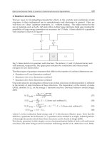
PV Diagrams. PV programs have a geometric representation. The PV diagram of the Swiss
flag program is shown in Figure 1.
The meaning of the diagram is that a schedule for the program is represented by a sequence
of arrows from the bottom left corner of the diagram, point
to the top right
corner, point
. Indeed, any possible schedule is a particular order of events (P or
V) of threads and . A schedule is shown in the diagram, drawn in solid arrows.
In this diagram the black circles indicate the "forbidden points", that is those that are not
possible in a schedule. For example, point (2,1) is forbidden because its associated
combination of actions,
, means that both threads lock resource at the same time,
which is not possible since
is a 1-semaphore. Consequently, we do not draw the arrows
that have black points as source or target. We draw in dotted line all the arrows that a
schedule could follow. The small black squares mark the squares of the diagram which are
"forbidden squares", which are the "expansion" of each forbidden point to the adjacent
upper-right little square. The "Swiss flag" name of the example comes from the cross form of
the union of these forbidden squares.
The advantage of such diagrams is that they allow to visualize special behaviours of a
program. In this example, we can see two special cases: point (1,1), which is a deadlock; and
point (3,3), which is an unreachable point.
A geometric approach to scheduling of concurrent real-time
processes sharing resources
325
Figure 1. The Swiss flag diagram; a schedule
2.1 PV Diagrams: Formal Definitions

We now formalize the above explanation and provide the basis for our subsequent
development of a timed version of PV programs and diagrams. We use partial orders to
model threads. When B is a partial order, we use the term "arc" or "arrow" to refer to an
element
', and we denote it by .
Orders
Resources. Shared resources are represented by a set of resource names. Each resource is
protected by a semaphore, which is represented with a function limit: . We
suppose that each resource has a finite limit, since this is the case which interests us. An
action (by a thread) is the locking or unlocking of a resource. If r
, the action of locking r
is denoted by P
r
, and the action of unlocking r is denoted by V
r
.
Threads. We consider a set of N threads, which we index with integers, for convenience: E
1
,
, E
N
. Each thread E
i
, is a partial order of events. A thread event e has one associated action.
We denote by act(e) the action associated with thread event e, for example act(e) = P
r
. The set
of events of thread i is denoted by
, and the order relation on it by
Ei

(also written
simply when no confusion is possible). This order is total (no branching considered in the
present study.) Each thread E
i
contains at least two events: its start event,
E
i
, which is the
bottom element of the order, and its end event,
E
i
, which is the top element of the order. The
threads we consider are well-behaved, in the sense that for each resource r , the thread
has form: B*(P
r
B*V
r
)*B*, where B is the set of actions P
r’
or V
r’
with r' r.
We say that thread i is accessing resource r at event e if and only if P
r
has occurred before or
at e, and the corresponding release V
r
occurs (strictly) after e. Formally, this is the case if
there exist an e'
e with act(e') = P

r
, and an e"with e e" and act(e") = V
r
such that e' e e",
and for all e''' with e' e''' e", act(e ''') P
r
, act(e''') V
r
.
The running together of N threads is formalized by the product of N partial orders, =
. We denote by the bottom (
E
1
, . . . ,
E
N
) of this partial order, and by its
maximum (
E
1
, . . . ,
E
N
). We denote by the order of . We will use letters , ', . . . to
Multiprocessor Scheduling: Theory and Applications
326
denote elements of . Given ,
i
is the event that belongs to thread
E

i
.
Forbidden Elements. For each element
of , and each resource a , we compute the
number of threads which access resource a at this element. A point is forbidden if there is at
least one resource to which the number of concurrent accesses is greater than its initial
semaphore value. Formally, the element
is forbidden if and only if
where if thread i is
accessing resource r at
i
, otherwise.
We denote by F the set of all forbidden elements of
, and we denote by (for "allowed")
the restriction of order to non-forbidden elements (elements of ).
Strings and Schedules. We use in the remainder of this paper the following notation: if e B
and e
B
, where B is a total order, then pred
B
(e) denotes the direct predecessor of e in B.
That is, pred
B
(e) e, and e' B : pred
B
(e) e' e e' = pred
B
(e). When the order B
considered is clear in the context, we will simply write pred(e).
Among arrows in relation , we distinguish the "small steps". An arrow is a

small step if :
i = 1, . . . , N : pred(
i
) '
i i
. For example, in the diagram of Figure 1, the
dotted arrows are small steps from .
Definition 1. A string s is subset of
, which forms a path from an element to an element
' with ', such that for each element " in s \ {e}, arrow is a small step. A
string which forms a path from to is called a schedule (for the program).
An element of a string is called state. From now on, the letter
will denote a schedule.
Geometric Realization Now we define the mapping of a program and its schedules to a
diagram and trajectories, which we call the geometrization mapping. The idea is to map the
set of schedules to trajectories inside an N-dimensional cube, going from the bottom left
corner (for ) to the top right corner (for ) of the cube. Since we want to stay in the
discrete world, we describe geometric realization in
. We use notation " " for the
mapping; hence, is the image of schedule by this mapping. We map threads E
i
onto a
subset of
as follows. Each event e of thread E
i
is associated with an ordinate c(e). The
ordinates are defined inductively as follows:
The order of E
i
is mapped onto the order between the integers c(e). We denote by the

resulting partial order . This mapping is clearly an isomorphism of
partial orders.
Mapping the Product of the Threads. Since is isomorphic to E
i
, the product of partial orders
is isomorphic to . We denote by this product: it is indeed
the geometrization of
. If looked onto an N-dimensional discrete Euclidian space, elements
of
are points of an N-dimensional grid. More precisely, the mapping sends every
to the point
. So for example, is (0, . . . , 0),
and
is .
Mapping Forbidden Elements and Strings. The set of forbidden elements
is mapped onto ;
has an intuitive form geometrically: if every point of lends a colouring of the adjacent
top right "little box" , then we see a union of N-dimensional boxes, which we call "forbidden
boxes" or forbidden regions.
A geometric approach to scheduling of concurrent real-time
processes sharing resources
327
As a sub-order of , any string is mapped onto , which is the set of points
of
, together with the order it inherits from . Geometrically schedules are trajectories
that avoid touching the front boundary of the forbidden boxes.
3. Timed PV Programs and Diagrams
In this section we present our timed version of PV programs and diagrams. This version
differs from existing versions of timed PV programs and diagrams [14, 10]. These latter
works are briefly presented in Section 7, where we also explain why we introduce a new

version of timed PV programs and diagrams.
3.1 Timed PV Programs
Our version of timed PV programs is an enrichment of untimed PV programs with a task
duration between any two consecutive events of each thread. This is motivated by
considerations of practical real-time programming, where one may measure the duration of
the execution of the program code between two events. Such measures are usually done to
foresee the worst case, so this duration is a worst-case execution time (WCET). After denning
our timed version of PV programs, our goal is to define the duration of a given schedule.
And then we aim at finding a quick schedule, in the sense of the schedule that makes the
execution of all threads finish as soon as possible.
Adding Duration of Tasks. In our definition of timed programs, we associate with each event e
in a thread E
i
the duration (the WCET) of the task, i.e., the part of the program code which is
performed between the direct predecessor of e and e. We denote by E the union
. The task durations are given in form of a function . We define
d(
E
i
) = 0 for each thread E
i
.
Example: the Timed Swiss Flag Program. A timed version of the Swiss flag program is as
follows:
Timed Schedules. A schedule in our timed version is, as in the untimed case, an order of
events of the threads.
3.2 Geometric Realization
We now define the mapping of a timed PV program and its schedules into a diagram and
trajectories. In principle, we could use the geometric realization for the untimed case, since
the involved orders are the same. However, it is more convenient to have a diagram where

one can visualize durations. To this end, we only have to change the ordinate function c as
follows. Each event e of thread E
i
, is associated with ordinate c(e). Ordinates are chosen so as
to visually reflect task durations in the Euclidian dimension (in one dimension). A special
case is tasks with zero duration, for which we choose a fixed length > 0 to represent the
order geometrically. The ordinates are defined inductively as follows:
Multiprocessor Scheduling: Theory and Applications
328
The order of E
i
is mapped onto the order between integers c(e) . We denote by the
resulting partial order
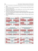
. The timed diagram for the timed Swiss Flag
program is shown in Figure 2 (with
= 1).
Figure 2. A timed schedule
3.3 3D Example: the Timed Dining Philosophers
We also give a timed version of the 3 philosophers problem. The philosophers, as usually,
have to get their left and right forks for eating. In the program forks are named
, , and :
the left fork of philosopher is , and its right fork is ; and so on. The forks are 1-
semaphores. We add a 2-semaphore for controlling an access to a small thinking room
which can contain no more than 2 philosophers at a time. Each philosopher thinks in the
thinking room, then walks to the eating room (which can contain the three philosophers),
and eats. Non-zero task durations are given for thinking, walking, and eating. The program
is the following:
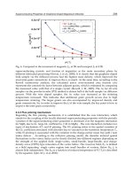
Then the trajectory for a schedule has to be taken in the cube shown in Figure 3 (a). We add
little white cubes to indicate the
and corners. The forbidden regions for the forks are the

three intersecting bars. The forbidden region for the thinking room is the cube at the bottom
left of the overall cube. We show also, in Figure 3 (b), the geometry of a more complex
version which has concurrent access to an anti-stress, and a small ashtray, etc.
A geometric approach to scheduling of concurrent real-time
processes sharing resources
329
a) b)
Figure 3. Forbidden regions of the three philosophers problem: (a) simple version;
(b) enriched version
3.4 Duration of Strings
Now we explain how the duration of a string (and hence of a schedule) is denned. We have
added durations between events, which are WCETs. The duration we consider for a string
corresponds to the case where all the tasks take their WCET as effective duration; thus the
duration of a string is its worst-case response time.
Waits. The computation of the duration can be understood in terms of a logic of waits. More
concretely, we assume that a thread could begin its tasks as soon as the necessary resources
are available. However, the real "permission" depends on the schedule under consideration.
For example, a thread A might be ready to begin a task after event e but is forced to wait
until another thread
performs an event e', if the schedule indicates that event e cannot
happen before event e'.
New Events. For convenience, we introduce the notion of new events along a schedule. New
events are the events that happen at an element in a string. Given a string s and an element
s, the set of new events, denoted by new
s
( ), that occur at along the string s is denned
as: if . If =
S
, then new
s

( )
is denned as
.
Algorithm to Compute the Duration of a String. Consider a string s (which can be a schedule).
The duration of string s, which we denote by d(s), is computed with the following algorithm.
The algorithm iterates over the states of the string, beginning at
S
and ending at
S
. Its
goal is to find "what time is at least at
S
" when time is 0 at
S
. To this end, the algorithm
uses clocks: N local clocks — one for each thread — , and one global clock. The global clock
is not indispensable, but eases the explanation. We call the variable for the global clock
,
and
the array (of size N) of the local clocks, with indices from is the local
clock for thread i. The algorithm is as follows.
• First all clocks, global and local, are initialized to 0.
• Then we iterate over the sequence of states of s, beginning from the element just above
its bottom element. For each element
of the sequence, do, in the following order:
1. Update the global clock according to all threads i that have a new event at
: for all i such that
i
new
s

( ).
Multiprocessor Scheduling: Theory and Applications
330
2. Update the local clocks of all threads i that have a new event at :
for all i such that
i
new
s
( ).
When element
S
has been processed, the algorithm returns the final value of which is the
duration of the string, d(s).
We explain the algorithm: when arriving at a state
one observes which events occur at this
state. Let i the index of a thread that has a new event at
.
(1) The last time an event of thread i happens is stored as value . Now, since that
point, time has elapsed by at least d(
i
) time units, since we now observe event
i
.
Therefore, the global time at state e must be at least
. So we update the
global clock accordingly. The "max" function is needed because it is possible that value
is in fact not greater than the last recorded. An example of this case is
given below.
(2) After the global clock has been updated in step (1), the local clocks of the threads that
have new events have to be synchronized. Indeed, we know that current time is now at

least
, so the local clocks are updated accordingly.
Example. The algorithm is illustrated with the schedule shown in Figure 2. The vector-like
annotations that accompany the trajectory indicate the values of the local clocks during the
execution. We have not indicated the global clock, since its value at one state is always the
maximum of the values of the local clocks. We execute the algorithm on the sequence of
states of the schedule, and we explain below what happens at some particular states. We
identify states by their coordinates in the diagram.
• State (1,0): at this state, a new event of thread A happens. Since only A has a new event,
the global clock is updated to max(0,0 + 1) = 1, and thread A updates its local clock to 1.
Hence the vector of local clocks is (1,0) at this state.
• State (4,1): at this state a new event happens to each thread A and B. The global clock
becomes 4, and both local clocks are updated. The schedule implies that action P
b
of
thread B does not happen before thread A performs V
b
. Since thread A runs for 4 time
units before executing V
b
, B cannot execute its action P
b
before that time point. The fact
that the local clock of B is updated to 4 shows that the soonest B can access b (with this
schedule) is at t = 4. So B has a lapse of 4 time units for executing its task of duration 1.
For example, if it executes this task immediately—beginning at date 0—, at global time
1 it has finished, it is forced to wait for 3 time units until A releases resource b.
• State (11,7): at this state, a new event of thread B happens. But the duration of the task
before this event is zero, so there is no change to be made.
The final value of the global clock is 11. This defines the WCRT for the considered schedule.

4. Abstraction of Efficient Schedules
4.1 The Scheduling Problem and Approach
We are interested in finding a quick schedule. Let us first assume that we are looking for the
quickest possible one (in the sense of a schedule has the minimal WCRT). We observe that
the approach of computing the duration for each possible schedule and then picking the
schedule with the minimal duration is not feasible in general. Indeed, the combinatorial
explosion comes not only from the number of possible states, but also from the total number
of possible schedules from bottom to top. If we also count the forbidden schedules (which
pass through forbidden regions), to simplify computations, we get the following numbers:
for the timed Swiss flag example, 6 x 6 = 36 states and 1683 possible schedules; for the timed
A geometric approach to scheduling of concurrent real-time
processes sharing resources
331
philosophers example, 8x8x8 = 512 states and 75494983297 possible schedules; for the
enriched version of the timed philosophers, 16 x 18 x 26 = 7488 states and more than 5 x 10
30
possible schedules.
1
Given this complexity problem, we propose to exploit the geometry of the diagrams to
construct abstractions that can make the computation of one or all shortest paths feasible. In
this section we define these abstractions, and we will describe in the next section a method
to compute them.
Eager Strings. We focus on a class of strings which is interesting w.r.t looking for efficient
schedules: eager strings are the strings that make no unnecessary wait—that is, a wait in the
string is necessarily induced by waiting for a locked resource to be unlocked.
Notice the difference between being eager and being the quickest schedule: while the
quickest schedule is necessarily eager, the converse is not true. For example, in the example
in Figure 1, a string from
to that goes above the cross could be eager, but will not be
optimal. Indeed, since thread A has to wait for the resources a and b to be unlocked by

thread B, the quickest string that goes above the cross will have duration 5 + 1 + 9 = 15 time
units.
We give also an example of a non-necessary wait in a schedule (which eager strings do not
have). In the time Swiss flag example a schedule with an unnecessary wait would go, for
example, through points (4, 0) and (9, 0) before going to (9,1): this corresponds to B waiting
for A to release resource a before accessing resource 6, while resource b is already available.
As a result, the local clocks in this case would be (9, 9) at point (9,1) and (9,12) at point (9, 5),
reflecting the time spent on waiting.
Studying eager strings, we are interested in what we call the critical exchange points: the
points where a resource is exchanged, and which border a forbidden region. Those are the
only points where a wait can be justified (or necessary). In the Swiss flag diagram critical
exchange points are indicated with the circled addition symbols.
In conclusion, an eager string waits only at critical exchange elements, and between any two
such elements makes no wait (since it would be unnecessary). Thus an eager string is
characterized by the critical points it passes through. We need to add
and in the set of
critical exchange points, since it is possible that a quickest schedule does not touch the
forbidden regions. This characterization of eager strings by critical exchange points is the
basis for our abstraction method for looking for efficient schedules. In the following we will
prove that looking only at critical exchange points is sufficient to construct an abstraction of
all the quickest schedules. To do so, we need first to introduce an abstraction of wait-free
strings.
Bows: Abstractions of Wait-Free Strings. In order to define abstractions for eager strings, we
first define abstractions for their wait-free parts. For this we introduce the notion bow.
Intuitively, a bow is an arc
from such that the longest side of the cube (in the
geometric realization) whose bottom left and top right corners correspond to e and e'is
equal to the duration of the quickest strings between e and e'.
We first introduce the abstraction which we will use for the duration of wait-free strings.
Definition 2. The distance between two elements

, ' with ' is defined as:
= , where for any thread E
i
and event
.

1
—5589092438965486974774900743393, to be precise.
Multiprocessor Scheduling: Theory and Applications
332
Note that s(e) c(e) in general: c(e) is the ordinate of e for the geometrization, while s(e) is
the "true ordinate" of e in term of the sum of the WCETs of the tasks. The case s(e) c(e)
when there is at least one e' e that has d(e') = 0: then s(e) < c(e).
We want to use arcs of
as abstractions of strings, so we introduce the following operation.
Definition 3. Given any arc
from , the stringing of , which we denote by ,
is the set of all the strings from to ' that have the smallest duration.
This set is not empty, since ' implies that there is a sequence of small steps from to '
in
. We call the tightened length of an arc from , the duration of any element of
. For simplicity of discussion we extend notation d, the duration of a string, to sets
of strings that have the same duration. Then the tightened length of
is written
d(
).
Now in abstracting wait-free strings, we want to be conservative with respect to looking for
the quickest schedule. So we look at arcs whose distance is not smaller than the duration of
the strings they could abstract.
Definition 4. A bow is an arc

from , such that and .
The height of a bow
is the distance . In fact, d( )
d(
) = . This is summarized as:
Lemma 1. For any bow
, d( ) = .
Proof: We want to prove that for any bow
, d( ) = .
Pick a string s in
. This string must execute, for each thread j, all of the tasks whose
durations are the
(see the definition of the duration of string) . Thus the
duration of s is greater than or equal to
. But the latter is (by
definition)
. Thus d( ) . We can conclude that d( ) =
.
Example. The notion of a bow is best explained on an example. Consider again the Swiss flag
diagram in Figure 2. Arc
(9, 0), (11, 6) is a bow, while arc (0, 1), (9, 8) is not. Indeed, the
latter arc has length
(0, 1), (9,8) = 9, while its tightened length is 11 (the quickest string
from (0, 1) to (9,8) exchanges resource b at point (2,7), and thread A has to wait for it for at
least 2 time units) .
Critical Potential Exchange Points. We define critical potential exchange points — the only
points where an eager string can wait. A potential exchange point is an element of
where a resource can be exchanged. That is, there exist at least one resource r
, and two
indices i,j, such that

i
= V
r
and
j
= P
r
. We use the term "potential" because in order to be a
real exchange point, it must be the element of a schedule
which has
.
Definition 5. A potential exchange point for a resource r with accessing(r,
) = limit(r) is called a
critical potential exchange point.
4.2 The Abstraction Graph
We are now ready to define our abstraction of all the eager strings (and hence also of all the
quickest schedules). It is the graph constructed from the critical potential exchange points,
having bows as arrows. We call it the abstraction graph.
We denote by C the union of all critical potential exchange points for the PV program with
. The abstraction graph is then denned as a relation , characterized by:
A geometric approach to scheduling of concurrent real-time
processes sharing resources
333
if and only if and is a bow. We label each arc of with a weight which is
.
Definition 6. A path p in graph G from an element
C to ' C is any sequence of critical exchange
points, p : {0, . . . , K} C, with p(0) = , p(K) = ' , and i {1, . . . , K} is a bow.
The length of a path p in G, denoted by l(p), is denned as
.

For
, ’ C with ', we denote by the set of the shortest paths from to ' ( '
ensures that the set is not empty). And by abuse of notation, we denote by l(
) the
length of any of the paths in
.
Example. We look again at the Swiss flag example in Figure 2. The critical potential exchange
points (except for
and ) are indicated by circled addition symbols. The arrows (of G)
between them are from (0,0) to (4,1), from (4,1) to (9,5), from (9,5) to (11,8); from (0,0) to (1,6),
from (1,6) to (2,7), from (2,7) to (11,8); and from (4,1) to (11,8) and from (1,6) to (11,8). Here
we see that a bow is not completely tied to the geometry: the last two bows, if represented as
line segments between the points in the space, do cross the forbidden region.
4.3 Property of the Abstraction Graph.
In the example of Figure 2, we see that the shortest path has length 4 + 5 + 2 = 11. The
following theorem states an important property of the graph G:
Theorem 1. The duration of a quickest schedule is the length of a shortest path in G.
More formally:
4.4 Proof of the Theorem 1
We first introduce some useful notions.
Abstraction. Abstractions of eager strings are paths. This is formalized here.
Definition 7. The pathing of a string s, which we denote by s , is the path which is constituted of
all the critical potential exchange points contained in s. This operation is authorized only if both
S
and
S
are critical potential exchange points, and s is eager.
The construction is correct: If s is an eager string, then s is a path in Proof:
Let s
: [0, ,K] C. We want to prove that for each i = l, ,K, . That

is, we want to prove: for any
Take i [1, . . . , K]. Between s (i — 1) and s (i), there is no critical potential exchange
point (otherwise it would have been included in the pathing). But critical potential exchange
points are the only elements which can induce a necessary wait, and the string, which is
eager, has waits only at critical exchange points. Thus between s (i — 1) and s (i) the
string has no unnecessary wait so its duration from elements s
(i — 1) to s (i) is exactly
the maximum of the tasks to be executed,
.
Concretization. The "reverse" operation of abstraction of strings, is concretization of paths of
G into strings.
Definition 8. The stringing of a path p : [0, , K] C from G, which we denote by p , is the set
of all the string from p(0) to p(K) which have the smallest duration and contain all points p(i), fori =
l, ,K-l.
This set is not empty, since a string from p(0) to p(K) can be constructed from the strings
from the sets , which are not empty since bows are arcs of
. For a path p from G, we denote by d(p ) its tightened length.
Multiprocessor Scheduling: Theory and Applications
334
Interaction of Abstraction and Concretization.
Lemma 2. Let , with , ’ C. Then there exists a string s which is such
that l(s
) = d(s).
In the following, a string s is said to be optimal if d(s) =
.
Proof: Pick a s in
(any s). This is possible, since and so the set s
is not empty. This string is optimal, so it is eager, so pathing is valid for it: s
is a
path in G. Let K be the number of elements in s

. That is: s : [0, , K] C. The proof is by
induction on K.
• Case K = 1. In this case, we have only one bow, . Since s is optimal,
. So by lemma 1,
= d(s). So the proposition is true
for K = 1, with this string s.
• Case K > 1. We want to prove that the property is true for K assuming it is true for K—1.
Element s
(K—1) is a critical potential exchange point. We look at what happens from
s
(K-1) to s (K). For one (or more) dimension k, —
, that is, the maximal sum of task durations between s (K—1) and s (K)is
for dimension k. Then there are two possible cases:
1. Thread k has a new event at s
(K—1).
Let be the value of the global clock at s (K—1). Then the global clock at s (K)
is
. Thus d(s) =
= . Then, using the recurrence hypothesis on
the subpath from s/ (0) to s/ (K — 1), one gets the desired property, with this string s.
2. Thread k has no new event at s
(K—1).
That is,
happens in s before s (K—1).
We construct a string s' from s, as follows: we substitute element s
(K—1) with
element
, where succ
s
( ) denotes

the successor of in the total order s. That is, string s' goes from
directly to an element where action
occurs.
(The proof that the new point is not k-forbidden is done by contradiction. Suppose that
it is the case, then thread k would have to go around a k-forbidden region (and wait)
between s
(K—1) and s (K), which is not possible since it is the "leader" thread for
this bow, i.e., k is the dimension that determines the distance between s
(K—1) and
s
(K).)
The substitution does not change the duration of the string. Indeed, only the dimension
k is affected, and thread k had no new event at s (K—1). Now there are two cases:
a) the substitution replaces a point of C with a point of
. Then K' = K — 1, and we
use the recurrence hypothesis to show that string s' satisfies the desired property.
b) the substitution replaces a point of C with another point of C. But at this new point
thread k has a new event. So the situation is as in case (1) but string s' replaces string s.
Conclusion: the proposition is true for K = 1 and K > 1, so it holds for all K
1.
Optimal Paths. A path p in G from to ' is said to be optimal if p .
Lemma 3. Let
, with e, ' C. If string s is such that l(s ) = d(s), then s
is an optimal path.
Proof: By contradiction. Existence of such a string s with l(s ) = d(s) is given by lemma 2.
Now suppose s
is not an optimal path. Then there exists an optimal path q from to '
A geometric approach to scheduling of concurrent real-time
processes sharing resources
335

with l(q) < l(s ). Then we get: d(s), which means that there are
strings from
to ' whose duration is smaller that of s, which is not possible by the
optimality of s. So s must be an optimal path.
Proof of theorem 1. We can now prove
.
Take
in , such that (which is possible by lemma 2). By lemma 3,
is optimal. Thus
.
An interesting computational implication of Theorem 1 is that the size of the graph G is
reasonable since the number of critical potential exchange points is much smaller than the
number of elements in ; hence the shorstest paths in G can be efficiently computed. We
will discuss this in more detail in the following section.
5. Finding Efficient Schedules using Geometric Realization
The construction of graph G has two parts: 1) find the critical potential exchange points; 2)
find the bows between these points. Then the shortest path in graph G is computed. Notice
that this approach automatically finds a deadlock-free path. Indeed, if a path in G leads to a
deadlock point, no bow goes from it; and a shortest path from
to is, above all, a path
from
to , and hence contains no deadlock.
We use geometry for the construction. Notice however that our method does not depend on
the coordinates c(e), in the sense that the function c of the untimed case would give the same
results. This is because we use the structure of the geometry of
(the forbidden boxes), not
the distances in the embedding. We use a function c which uses d(e) only for visual intuition
(the "max" measure is still close to the Euclidian distance).
Notice that is it possible, after we have found a satisfying path p in G, to actually construct an
eager string abstracted by this path. The construction operates bow by bow. For one bow

the quickest string abstracted by it is one that just makes no unnecessary wait, so a
possible procedure is to start from and to pick the adjacent small step to an " which
increases the least the duration (there may be several), among those that have not
in one of the dimensions i.
5.1 Computing the Critical Potential Exchange Points
The critical potential exchange points are given by some points on the boundary the
forbidden regions: in dimension 2, these are the bottom-right and top-left points of the
forbidden regions; in dimension 3, all points on some edges of the boundary; etc. The formal
characterization of this geometric aspect of critical potential exchange points is
straitforward.
Computing the Forbidden Regions. In this section we describe briefly the algorithm we use to
compute the forbidden regions from the timed PV program. Clearly checking for each
element whether it is forbidden is not a reasonable approach. We use instead the access
intervals of the threads. A thread E
i
, creates an access interval when it accesses resource r (P
r
)
at an event e, and releases it some time after (V
r
), at event e' e: this access interval is stored
as the triplet of integers (i, c(e), c(e')). Moreover the algorithm proceeds resource by resource:
for each resource r , we compute the forbidden regions created by access to r by more
than limit(r) threads concurrently. This set R
r
is computed as follows.
1. For each thread E
i
construct the set accesses(r,i) of access intervals by i to resssource r.
Multiprocessor Scheduling: Theory and Applications

336
2. Then for efficiency we proceed as follows. First we determine the abstract occurrences of
forbidden concurrent accesses. This is when there are more than limit(r) accesses
concurrently to resource r. So, from the set of all sets accesses(r, i) which are not empty
(this set contains m
N elements), we compute its subsets of cardinal limit(r) + 1: those
are the abstract occurrences.
3. Then we compute the concrete occurrences of forbidden concurrent accesses from each
abstract one, by combining the access intervals. When the cardinal of a concrete
occurrence is less than N, it means that one (or more) thread(s) k are not concerned by
this forbidden concurrent access: then dimension k is added as access interval
, because geometrically the forbidden access holds for all ordinates
of k. This each concrete occurrence defines the coordinates of an N-dimensional box.
In step (2) of the procedure, computing the parts with a cardinal greater than limit(r) + 1 is
not necessary because those occurrences are included (geometrically) in the regions
computed for the (limit(r) + 1)-occurrences.
Example. We consider the three philosophers program of page 6. We compute the forbidden
regions for resource
. Suppose threads , and have respective indices 1, 2 and 3. (1) We
get: accesses(
, 1) = , accesses( , 2) = {(2,22,28)}, accesses( , 3) = {(3,19,22)}. (2) The non-empty
sets among those are {(2,22,28)} and {(3,19,22)}. Since limit( ) = 1, the abstract occurrences
must have cardinal 2. There is only one such abstract occurrence here: {{(2, 22, 28)}, {(3,19,
22)}}. (3) This abstract occurrence of a forbidden access results in a single concrete
occurrence
{(1,0, 28), (2, 22, 28), (3,19, 22)}
which defines a 3-dimensional box whose bottom and top vertices are (0, 22,19) and (28,
22,19) respectively.
5.2 Finding the Arrows of the Abstraction Graph
From the forbidden boxes we can compute the critical potential exchange points, which are

the nodes of the abstraction graph G. But it remains to compute the bows between the
critical potential exchange points. A simple method to determine whether an arc
is a
bow is to determine the tightened length of the arc by enumerating all the strings from to
’ and then check the condition of Definition 4. However, this method is clearly very
expensive and, to remedy this, we will exploit some properties of the geometrization.
We use a method which uses some arcs which are necessarily bows: we use a decomposition
of forbidden-point-free regions. Using this approach we may not find a quickest schedule
but we can find a good schedule. This decomposition approach and the strategies for
looking for the quickest schedule are discussed in the following.
Finding Efficient Schedules using Decomposition. We denote
.
In
, , that is the image by the geometrization mapping of the product of all the
threads, forms a (non- uniform) N-dimensional grid over the box B. A potential exchange
point
corresponds to a grid point, denoted by ; therefore, a bow corresponds to a line
segment connecting two grid points, and a path in the graph G corresponds to a sequence of
such line segments. It is important to note that while the graph G is used to model the
schedules with the shortest duration, it does not capture resource conflicts. Consequently, to
construct the graph G we need to consider the bows which do not cause a resource conflict.
In this geometric setting, the forbidden regions is a union of boxes whose vertices are grid
A geometric approach to scheduling of concurrent real-time
processes sharing resources
337
points. This union is indeed an orthogonal polyhedron [5], denoted by P
F
. Let P
A
= \ P

F
denote the allowed polyhedron. We now make the following observation: if a box contains no
forbidden points, then any two points on its boundary form a bow if there are grid points.
Indeed, intuitively, the line segment between them does not intersect polyedron P
F
. This
motivates considering a decomposition of the polyedron P
A
.
Definition 9 (Decomposition). We define a decomposition of an orthogonal polyhedron P as a
set where each B
i
(i {1, . . . , k}) is a full- dimensional box such that the
following conditions are satisfied:
1. For all i
{1, . . . , k} the vertices of B
i
are grid points.
2.
3. For all i, j
{1, . . . , k}, i j, the boxes B
i
and B
j
are non- overlapping, that is their interiors do
not intersect with each other.
Note that the vertices of the boxes in a decomposition are not necessarily critical exchange
points. If all the vertices of a box are grid points then it is called grid box. Additionally, if a
grid box does not contain any other grid boxes, then it is called elementary box. We will use in
the sequel two types of decompositions that we call elementary and compact. Given a

decomposition
, is called elementary if all B
i
are elementary boxes;
is called compact if there exists no pair of B
i
and B
j
with i j such that Bi Bj is a grid
box. Intuitively, in a elementary decomposition none of its boxes can be split into smaller
grid boxes, and in a compact decomposition no pair of its boxes forms a grid box. Note that
there exists a unique elementary decomposition of a given orthogonal polyhedron, however
there may be many different compact decompositions.
We now show how to use decompositions to construct the abstraction graph G. Let
be
a decomposition of the allowed polyhedron P
A
. We first recall the observation we use to
reduce the complexity of the search for bows: a line segment connecting two vertices of a
box B
i
which are critical exchange points corresponds to a bow (since it is a direct
path which does not cross the forbidden polyhedron P
F
). It is however clear that even when
is the elementary decomposition, the set of all such edges does not allow to cover all
possible bows since two vertices of two different boxes might also form a bow. However, if
our goal is to find one path with the shortest duration that respects resource constraints, it is
not necessary to construct the whole graph G but we need to include all the bows that form
such a path. It can be proved that there exists a decomposition such that the vertices of its

boxes are enough to discover a shortest path. We call such a decomposition an effective
decomposition, and it is of great interest to find such a decomposition, which is our ongoing
work. Other possible heuristics to approach such decomposition is discussed in the next
paragraph.
We finish this section by briefly describing our current method for computing a compact
decomposition of orthogonal polyhedra. The essential idea of the method is as follows.
From a given starting box we try to merge it with other elementary boxes, along one or more
axes, so as to maximize the volume of the resulting box. To do so, we make use of the
efficient algorithms for Boolean operations and membership testing developed based on a
compact and canonical representation of such polyhedra (see [5]). In some cases, the
criterion of maximizing the volume of merged boxes may not be the best one with respect to
including the shortest path in the graph. Alternative criteria are merging as many as
possible boxes along a fixed axis. Intuitively, a shortest path tends to approach the diagonal
between the bottom left and top right corners of the box B while avoiding the forbidden
Multiprocessor Scheduling: Theory and Applications
338
regions; hence, we can combine different merging criteria depending on the relative position
to the forbidden regions.
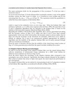
5.3 Experimental Results
We demonstrate in this section the effectiveness of our method. We have written a
prototype which implements the exposed method. For computing the forbidden regions we
use a program written in the language Maude [6] and executed with the Maude system. The
execution time for computing the forbidden regions is negligible. The program for the
decomposition (construction of allowed boxes from the forbidden boxes), the construction of
the abstraction graph from the allowed boxes, and the search of the shorstest path in this
graph is written in C++. The construction of the allowed boxes from the forbidden ones is
rather quick, and most of the time in the execution of this program is spent in the
construction of the graph from the allowed boxes—due to the number of vertices we use, as
we explain below. We present in the table below some experiments with this program.
We first test with the philosophers problem, in 3 dimensions and more. That is, we use N

forks—one per philosopher—and one thinking room which can take only N — I
philosophers. Then we take the same program, but with a thinking room which can contain
only half the philosophers ("phil. s.th r" is for "philosophers with small thinking room").
Program "enr. phil." is the enriched version of the philosophers problem whose geometry is
shown in Figure 4 (b). Program "more enr. phil." is when we add still more actions to this
enriched version. Program "enr. phil. 4D" is when we add a fourth philosopher to the
enriched version. Program "3 phil. 2 procs" is the program of Section 6, whose geometry is
shown in Figure 4. In the table, "na" stands for "not available"—the computation was not
finishing in less than 10 minutes. We have used a PC with a Xeon processor of 2.40 GHz
frequency, 1 Go of memory and 2 Go of swap.
program dim #states #forbid #allowed #nodes #edges t (sec.)
3 phil. 3 512 4 35 151 773 0.58
4 phil. 4 4096 5 107 743 7369 17.38
5 phil. 5 32768 6 323 3632 67932 571.12
6 phil. 6 262144 7 971 na na na
3 phil. s.th r. 3 512 6 59 227 1271 1.50
4 phil. s.th r. 4 4096 8 199 1147 13141 60.24
5 phil. s.th r. 5 32768 15 1092 na na na
6 phil. s.th r. 6 262144 21 3600 na na na
enr. phil. 3 7488 26 390 1468 7942 51.01
more enr. phil. 3 29568 137 1165 4616 30184 461.18
enr. phil. 4D 4 119808 44 5447 na na na
3 phil. 2 procs 3 1728 12 78 352 2358 2.56
A geometric approach to scheduling of concurrent real-time
processes sharing resources
339
One can observe that the number of allowed boxes is very reasonable compared with the
number of states. The number of nodes reflects the fact in our current prototype, we add in
the graph some of the vertices of the allowed boxes which are not critical exchange points, to
compensate for the fact that we do not currently include inter-allowed-box bows: thus we

can find paths whose length approximate (conservatively) the weight of such inter-box
bows. The advantage of this approach is that any decomposition can serve to find a
relatively good schedule. Its inconvenient is that the number of considered vertices for a box
is of order 2
N
. Thus the number of threads considered is the main obstacle in our current
implementation.
We find good schedules: in the case of the 3 philosophers program of Sec. 3.3, the durations
of the threads are 24, 25 and 20 respectively, and the found schedule has duration 39, which
is good. In the case of the enriched version of Fig. 3(b), the threads have respective durations
83, 94, and 95, and the found schedule has duration 160, which is also good in view of the
many forbidden regions which bar the direct way.
Our future experiments will use the following heuristics: using, for each box in the
decomposition, only its bottom and top elements. Intuitively, quick schedules follow
diagonals, so this heuristics could be useful. It addresses the main obstacle of our method—
the number of vertices considered per allowed box (we descend from 2
N
points per box to
only 2). On the other hand, how close one then gets to the quickest schedule depends on the
decomposition, as discussed in the previous section.
6. Limited Number of Available Processors
The Problem. We have defined the WCRT of a schedule assuming that the threads run
concurrently. But in concrete terms, this implies that N processors are available. It might be
possible that less than N are needed, for example when thread migration is allowed and
N—1 processors are enough for this schedule because the schedule has some particular
waiting patterns. Therefore the true question is: what does the WCRT of the schedule
become when there are only M < N processors available?
The problem of denning the mapping of the N threads (or processes) onto M processors, that
we call the thread distribution mapping, has already been treated in [7]. But this is in the
untimed context, and aims at building a scheduler that avoids deadlock states. We are

looking not only for safe schedules using a limited number of processors, but also efficient
schedules.
We distinguish two approaches: 1) first compute an efficient schedule with the method
shown in the previous section; and then compute a good mapping of this particular
schedule onto M < N processors. The advantage of this approach is that it separates "abstract
scheduling" and mapping. The inconvenient is that there may be some schedules that were
not considered efficient in the abstract world, but that could do very well on M < N
processors. 2) Integrating the mapping problematics into the model, and computing an
efficient schedule that takes this constraint into account. The advantage of this approach is
that it is more precise. But it can also lead to state explosion, as we discuss in the following.
In this section we examine the second solution, because it gives some geometric intuition on
the mapping, and in addition, for many practical cases the complexity of the computation is
reasonable.
A Solution. The idea is to model the resource limitation in terms of available processors, as a
M-semaphore. This modelling assumes that the threads have no preference on which
Multiprocessor Scheduling: Theory and Applications
340
processor to run on. This is reasonable in the case of a homogeneous architecture—all the
processors are the same. It also ignores issues to communication optimisation, so it
implicitly assumes a shared memory architecture. The advantage of using a semaphore is
that it makes a drastic combinatorial simplification: when 2 threads A and B, among a pool
of 3 concurrent threads A, B, C, are running on 2 processors p
1
and p
2
, we do not have to say
whether A is running onto p\ and B onto p% or vice-versa. Knowing that A and B are
running, and not C, is what interests us from the point of view of scheduling. The effective
distribution of the threads onto the processors can then be done statically, or at run time, but
in any case, after we have already determined the schedule.

We use a manual locking and releasing of a processor in a PV program. This corresponds to
manual proposition of preemption: the programmer decides when a thread gives a chance
to other threads of taking the processor. If the schedule which is eventually chosen does not
use this preemption opportunity, then of course in the implementation of this schedule the
thread does not need to preempt itself.
Example. As an example we use the simple version of the three philosophers problem. Here
the programmer decides that a philosopher keeps the processor for thinking and walking to
the eating room, and before entering the thinking room makes a proposition of preemption
so as to give the opportunity for other threads to get the processor. We denote by
the
semaphore for the processors. The program of philosopher is modified as follows (the
modification is similar for philosophers and ):
The geometry of the new program is shown in Figure 4. We see that a trajectory must go
through the "canyons" between the p-forbidden boxes, as well as avoiding the parts of the
previous forbidden regions that still emerge from these new boxes. Notice that the room-
forbidden box is now included in the bottom left -forbidden box. Indeed, the room
semaphore served to forbid acces to the room by more than two philosophers, which is no
longer necessary.
Figure 4. Forbidden regions of the three philosophers problem with two processors
A geometric approach to scheduling of concurrent real-time
processes sharing resources
341
Limitations of the Approach. Remark that since each philosopher accesses 2 times a processor
(through a lock of semaphore ), we indeed get 2
3
= 8 boxes that form the corresponding
forbidden regions. Computationally, it means that a thread should not propose preemption
too often. On the other hand, finding the optimal schedule "for all possible preemptions"
would imply, on the contrary, proposing a preemption between each event of the original
program (which can be done automatically). But this would induce an exponential number

of forbidden regions (
-forbidden regions).
On the other hand, this geometric approach can give new ideas for optimizations of the
control of programs that run on a limited number of processors. For example, in the
previous example, the geometry indicates that, in the given preemption is implemented,
then the implementation can dispense with the semaphore.
7. Related Works
Timed PV Diagrams. Some other versions of timed PV diagrams have been proposed. We
have not used them, for the reasons we explain below.
• The work [10], which presents a timed version of PV programs and diagrams, attempts
to model multiple clocks, as in timed automata [4]. In the present paper we do not use
the timed automaton model. Moreover, in the approach of [10] time is modeled as an
additional dimension—one per clock. Thus, with one clock and three threads, a 4-
dimensional space is studied. In this paper we consider each thread (or process)
dimension as a "local time dimension", and then define the synchronization of local
time dimensions.
• The work [14] exploits the dimension of each process as a time dimension. In this
aspect, this work is close to ours. However there are important differences. First, the
definitions in [14] are given in a continuous setting, and therefore topological spaces are
considered, such that the duration of a schedule is described with an integral. In our
work we stay in a discrete domain, an the definition of the duration of a schedule is
given by an algorithm on a discrete structure. On the other hand, the fact that the
definitions in [14] are tied to geometry implies, in particular, that zero-delays between
two consecutive actions in a process (for example two successive locks, which often
happens in programs that share resources) are not possible since the two actions would
be the same in the geometry. In our approach, while we exploit the geometry to
construct abstractions, the notion of duration itself is not geometric. Consequently,
zero-delays are possible. This is of particular interest if one considers that the practical
delay, on most architectures, between two consecutive locks, is too small to be modelled
as a non-zero value. We conjecture that our version of timed PV diagrams is a

discretized version of the continuous version of [14] (in the case of no zero-delays in the
program).
Timed Automata. A large class of real-time systems can be adequately modelled with timed
automata [4], and in this framework the problem of scheduling has been addressed [3,1,
2,16,17], often closely related to the context of controller synthesis. A timed PV program has
a direct representation using timed automata. First, each thread is modelled as an
automaton, where each node represents an event, and each transition from node e to node e'
is labeled with constraint "i > d(e'y plus a reset of the clock. The global automaton is the
product of all the thread-automata. Semaphores can be represented via variables. Such a
Multiprocessor Scheduling: Theory and Applications
342
product of automata is very close to that of [16], where the aim is also to schedule multi-
threaded programs. In this work a scheduler is constructed to guarantee that a schedule does
not go into deadlock states or deadline-breaking directions. We look for a complete schedule
which is not only safe but also efficient; however our model is not as rich as the timed
automata model: we have not yet included deadlines, branching, and looping.
Scheduling and the Polytope Model. Another geometry-based method for scheduling
concurrent programs is the polytope model (see, e.g., [8]), which is used in the context of
automatic par-allelization. However the semantics of the points in the geometric space is not
the same as in PV diagrams: each point inside a polytope represents a task which has to be
executed, while in PV diagram each point is a possible state and only a very small number
of these states have to be represented in the implementation. Also the polytope model does
not consider resource sharing, and has no task durations.
8. Conclusion and Future Work
In this paper, we denned a timed version of PV programs and diagrams which can be used
to model a large class of multithreaded programs sharing resources. We also introduced the
notion of the worst-case response time of a schedule of such programs. This framework was
then used to find efficient schedules for multithreaded programs. In particular, to tackle the
complexity problem, we define an abstraction of the quickest schedules and we show how
to exploit the geometry of PV diagrams to construct this abstraction and compute efficient

schedules as well as a quickest one. This work demonstrates an interesting interplay
between geometric approaches and real-time programming. An experimental
implementation allowed us to validate the method and provided encouraging results.
Our future work will explore the following directions.
• When developing a real-time system one is often interested in the worst-case response
time of the whole program, if it is part of a larger system, for any schedule. As a
definition, this WCRT could be given as the duration of the eager schedule that has the
longest duration. We conjecture that we could use abstraction graph G for computing
the longest eager schedule by computing the longest path in a subgraph of G. Defining
this subgraph is a topic of our future research.
• We are able to find schedules, but it remains to see how they can be implemented. An
obvious solution is controlling the computed schedule so as to enforce exactly the order
of events it describes. But an interesting question is: among those control points, which
can we "forget" while guaranteeing that the real execution will not diverge from the
planned schedule as far as critical exchanges of resources are concerned? Indeed, in
practice tasks can take less time than the WCET: control is needed for ensuring that
such behaviour does not make the trajectory follow a direction which does not
correspond to the schedule.
• We are currently investigating the problem of adding deadlines in our model. This
extension is not straightforward since the "symmetry" with the definition of a lower
bound to the duration spent by a thread between two consecutive events (the WCET of
the task) is not trivial. We also intend to examine the possibility of lifting to the timed
case the existing studies on the geometry of loops [12] or branching (if-then-else
constructs) in PV programs.
A geometric approach to scheduling of concurrent real-time
processes sharing resources
343
• Another approach to treat deadlines is to integrate our geometric abstractions into
existing tools that use timed automata, such as [16]. These tools suffer from the problem
of state explosion. Since our model is close to a product of automata, integrating our

geometric approach into these tools could allow to handle larger systems.
9. References
Y. Abdeddaïm and O. Maler. Job-shop scheduling using timed automata. In Proceedings of
the 13th International Conference on Computer Aided Verification (CAV 2001), LNCS
2102, pages 478-492. Springer Verlag, 2001.
K. Altisen, G. Göǃiler, and J. Sifakis. Scheduler modelling based on the controller synthesis
paradigm. Journal of Real-Time Systems, (23):55-84, 2002. Special issue on control-
theoretical approaches to real-time computing.
R. Alur, S. La Torre, and G. Pappas. Optimal paths in weighted timed automata. In
Proceedings of Fourth International Workshop on Hybrid Systems: Computation and
Control, LNCS 2034, pages 49-62, 2001.
Rajeev Alur and David L. Dill. A theory of timed automata. Theoretical Computer Science,
126(2):183-235, 1994.
Olivier Bournez, Oded Maler, and Amir Pnueli. Orthogonal polyhedra: Representation and
computation. In Proceedings of Hybrid Systems: Computation and Control (HSCC'99),
LNCS 1569, pages 46-60. Springer Verlag, March 1999.
Manuel Clavel, Francisco Durán, Steven Eker, Patrick Lincoln, Narciso Martí-Oliet, José
Meseguer, and Carolyn Talcott. Maude 2.0 Manual — Version 1.0. SRI International,
June 2003.
R.egis Cridlig and Eric Goubault. Semantics and analysis of Linda-based languages. In
Proceedings of WSA'93, LNCS 724. Springer Verlag, 1993.
Alain Darte, Yves Robert, and Frederic Vivien. Scheduling and Automatic Parallelization.
Birkhauser, Boston, 2000.
E. W. Dijkstra. Co-operating sequential processes. In F. Genuys, editor, Programming
Languages, pages 43-110. Academic Press, New York, 1968.
Ulrich Fahrenberg. The geometry of timed PV programs. In Patrick Cousot, Lisbeth Fajstrup,
Eric Goubault, Maurice Herlihy, Martin R.aussen, and Vladimiro Sassone, editors,
Electronic Notes in Theoretical Computer Science, volume 81. Elsevier, 2003.
Lisbeth Fajstrup, Eric Goubault, and Martin Rausen. Detecting deadlocks in concurrent
systems. In International Conference on Concurrency Theory, pages 332-347, 1998.

Lisbeth Fajstrup and Stefan Sokolowski. Infinitely running concurrent processes with loops
from a geometric viewpoint. In Patrick Cousot, Eric Goubault, Jeremy
Gunawardena, Maurice Herlihy, Martin Raussen, and Vladimiro Sassone, editors,
Electronic Notes in Theoretical Computer Science, volume 39. Elsevier, 2001.
Éric Goubault. Schedulers as abstract interpretations of higher-dimensional automata. In
Proceedings of PEPM'95 (La Jolla). ACM Press, June 1995.
Éric Goubault. Transitions take time. In Proceedings of ESOP'96, LNCS 1058, pages 173-187.
Springer Verlag, 1996.
Éric Goubault. Geometry and concurrency: A user's guide. Mathematical Structures in
Computer Science, 10(4), August 2000.
Multiprocessor Scheduling: Theory and Applications
344
Christos Kloukinas, Chaker Nakhli, and Sergio Yovine. A methodology and tool support for
generating scheduled native code for real-time Java applications. In Rajeev Alur
and Insup Lee, editors, Proceedings of the Third International Conference on Embedded
Software (EMSOFT 2003), LNCS-2855, pages 274-289, October 2003.
J. I. Rasmussen, K. G. Larsen, and K. Subramani. R.esource-optimal scheduling using priced
timed automata. In Proceedings of the tenth International Conference on Tools and
Algorithms for the Construction and Analysis of Systems (TACAS 2004), pages 220-235,
2001.