Parallel Manipulators New Developments Part 14 docx
Bạn đang xem bản rút gọn của tài liệu. Xem và tải ngay bản đầy đủ của tài liệu tại đây (649.14 KB, 30 trang )
Singularity Robust Inverse Dynamics of Parallel Manipulators
381
11 313 11 313
22 424 22 424
T
313 313
424 424
10
01
00
00
rs rs rc rc
rs rs rc rc
rs rc
rs rc
−− +
⎡
⎤
⎢
⎥
+−−
⎢
⎥
=
⎢
⎥
−
⎢
⎥
−
⎢
⎥
⎣
⎦
A
(35)
The drive singularities are found from
0
=
A as
1324
sin( ) 0
θ
θθθ
+
−− =, i.e. as the
positions when points A, B and D become collinear. Hence, drive singularities occur inside
the workspace and avoiding them limits the motion in the workspace. Defining a path for
the operational point P which does not involve a singular position would restrict the motion
to a portion of the workspace where point D remains on one side of the line joining A and D.
In fact, in order to reach the rest of the workspace (corresponding to the other closure of the
closed chain system) the manipulator has to pass through a singular position.
When the end point comes to
0.80m
d
sL
=
= ,
13
θ
θ
+
becomes equal to
24
π
θθ
+
+ , hence a
drive singularity occurs. At this position the third row of
T
A becomes
34
/rr times the
fourth row. Then, for consistency of equation (8), the third row of the right hand side of
equation (8) should also be
34
/rr times the fourth row. The resulting consistency condition
that the generalized accelerations must satisfy is obtained from equation (15) as
333
31 1 24 2 33 3 44 4 3 4
444
rrr
M
MM MRR
rrr
θθθθ
−+−=−
(36)
Hence the time trajectory s(t) of the deployment motion should be selected such that at the
drive singularity the generalized accelerations satisfy equation (36).
An arbitrary trajectory that does not satisfy the consistency condition is not realizable. This
is illustrated by considering an arbitrary third order polynomial for
()st having zero initial
and final velocities, i.e.
23
23
32
()
Lt Lt
TT
st =−. The singularity position is reached when
0.48st = . The actuator torques are shown in Figure 2. The torques grow without bounds as
the singularity is approached and become infinitely large at the singular position. (In Figure
2 the torques are out of range around the singular position.)
For the time function s(t), a polynomial is chosen which satisfies the consistency condition at
the drive singularity in addition to having zero initial and final velocities. The time
d
T
when
the singular position is reached and the velocity of the end point P at
d
T , ()
Pd
vT can be
arbitrarily chosen. The loop closure relations, the specified angle of the acceleration of P and
the consistency condition constitute four independent equations for a unique solution of
,1, ,4
i
i
θ
=
at the singular position. Hence, using
i
θ
and
i
θ
at
d
T , the acceleration of P at
d
T
,
()
Pd
aT
is uniquely determined. Consequently a sixth order polynomial is selected
where
(0) 0,s = (0) 0,s
=
() ,sT L
=
() 0,sT
=
() ,
dd
sT L
=
() ()
dPd
sT v T
=
and () ()
dPd
sT a T=
.
d
T
and
()
Pd
vT
are chosen by trial and error to prevent any overshoot in s or s
. The values
used are
0.55 s
d
T = and ()3.0m/s
Pd
vT
=
, yielding
2
( ) 18.2 m/s
Pd
aT=
.
s(t) so obtained is
given by equation (37) and shown in Figure 3.
Parallel Manipulators, New Developments
382
23456
( ) 30.496 154.909 311.148 265.753 81.318stttttt=− + − +
(37)
Figure 2. Motor torques for the trajectory not satisfying the consistency condition: 1.
T
1
, 2.
T
2
Furthermore, even when the consistency condition is satisfied,
T
A is ill-conditioned in the
vicinity of the singular position, hence
τ cannot be found correctly from equation (8).
Deletion of a linearly dependent equation in that neighborhood would cause task violations
due to the removal of a task. For this reason the modified equation (17) is used to replace the
dependent equation in the neighborhood of the singular position. The modified equation,
which relates the actuator forces to the system jerks, takes the following form.
rr r r
AA AA M MM M
rr r r
τ
τθ θθ θ
−+−=−+−
TT TT
33 3 3
31 41 1 32 42 2 31 1 24 2 33 3 44 4
44 4 4
()()
333
31 1 24 2 33 3 44 4 3 4
444
rrr
M
MM MRR
rrr
θθθθ
+− +− −+
(38)
The coefficients of the constraint forces in eqn (38) are
TT
3
31 41 3 1 3 13 3 2 4 24
4
()()
r
AAr cr c
r
θθ θθ
−=−+−+
(39a)
TT
3
32 42 3 1 3 13 3 2 4 24
4
()()
r
AAr sr s
r
θθ θθ
−=−+−+
(39b)
which in general do not vanish at the singular position if the system is in motion.
Once the trajectory is chosen as above such that it renders the dynamic equations to be
consistent at the singular position, the corresponding
i
θ
,
i
θ
and
i
θ
are obtained from
inverse kinematics, and when there is no actuation singularity, the actuator torques
1
T and
Singularity Robust Inverse Dynamics of Parallel Manipulators
383
2
T (along with the constraint forces
1
λ
and
2
λ
) are obtained from equation (8). However in
the neighborhood of the singular position, equation (22) is used in which the third row of
equation (8) is replaced by the modified equation (38). The neighborhood of the singularity
where equation (22) is utilized is taken as
1324
180 1
oo
θθθθ ε
+
−−− <=. The motor torques
necessary to realize the task are shown in Figure 4. At the singular position the motor
torques are found as
1
138.07NmT
=
− and
2
30.66NmT
=
− . To test the validity of the
modified equations, when the simulations are repeated with
0.5
o
ε
= and 1.5
o
ε
= , no
significant changes occur and the task violations remain less than
4
10
−
m.
Figure 3. Time function satisfying the consistency condition.
4.2 Three degree of freedom 2-RPR planar parallel manipulator
The 2-RPR manipulator shown in Figure 5 has 3 degrees of freedom (n=3). Choosing the
revolute joint at
D for disconnection (among the passive joints) the joint variable vector of
the open chain system is
[]
T
11223
θ
ζθζθ
=η , where
1
AB
ζ
=
and
2
CD
ζ
=
. The link
dimensions of the manipulator are labelled as
aAC
=
, bBD
=
, cBP
=
and PBD
α
=∠ . The
position and orientation of the moving platform is
[]
T
3
PP
xy
θ
=x where
P
x ,
P
y are the
coordinates of the operational point of interest
P in the moving platform.
The velocity level loop closure constraint equations are
G
=
Γη 0
, where
11 122 2 3
11 122 2 3
sin cos sin cos sin
cos sin cos sin cos
G
b
b
ζ
θθζθ θ θ
ζ
θθζθ θ θ
−−−
⎡
⎤
=
⎢
⎥
−−
⎣
⎦
Γ
(40)
The prescribed position and orientation of the moving platform,
()tx represent the tasks of
the manipulator. The task equations at velocity level are
P
=
Γη x
where
Parallel Manipulators, New Developments
384
11 1 3
11 1 3
sin cos 0 0 sin( )
cos sin 0 0 cos( )
00001
P
c
c
ζ
θθ θα
ζ
θθ θα
−−+
⎡
⎤
⎢
⎥
=+
⎢
⎥
⎢
⎥
⎣
⎦
Γ (41)
Figure 4. Motor torques for the trajectory satisfying the consistency condition: 1.
T
1
, 2.T
2
.
Figure 5. 2-RPR planar parallel manipulator.
Let the joints whose variables are
11 2
,and
θ
ζζ
be the actuated joints. The actuator force
vector can be written as
[]
T
112
TFF=T where
1
T is the motor torque corresponding to
s
5
4
G
2
G
5
G
1
G
1
3
x
y
o
P
γ
1
θ
2
θ
A
C
Singularity Robust Inverse Dynamics of Parallel Manipulators
385
1
θ
, and
1
F and
2
F are the translational actuator forces corresponding to
1
ζ
and
2
ζ
,
respectively. Consider a deployment motion where the platform moves with a constant
orientation given as
o
3
320
θ
= and with point P having a trajectory s(t) along a straight line
whose angle with x-axis is
o
200
γ
= , starting from initial position m0.800
o
P
x = ,
m0.916
o
P
y = (Figure 5). The time of the deployment motion is s1T
=
and its length is
m1.5L = . Hence the prescribed Cartesian motion of the platform can be written as
o
3
() ()sin
() ()cos
()
320
o
o
PP
PP
xt x st
yt y st
t
γ
γ
θ
⎡
⎤
+
⎡⎤
⎢
⎥
⎢⎥
==+
⎢
⎥
⎢⎥
⎢
⎥
⎢⎥
⎣⎦
⎣
⎦
x
(42)
The link dimensions and mass properties are arbitrarily chosen as follows. The link lengths
are
m1.0AC a== , m0.4BD b
=
= , m0.2BP c
=
= , 0PBD
α
∠
==. The masses and the
centroidal moments of inertia are
kg
1
2m
=
, kg
2
1.5m
=
, kg
3
2m
=
, kg
4
1.5m
=
, kg
5
1.0m = ,
kg m
2
1
0.05I = , kgm
2
2
0.03I = , kg m
2
3
0.05I = , kgm
2
4
0.03I = and kg m
2
5
0.02I = . The mass
center locations are given by
m
11
0.15AG g
=
= , m
22
0.15BG g
=
= , m
33
0.15CG g== ,
m
44
0.15DG g== , m
55
0.2BG g
=
= and
5
0GBD
β
∠
==.
The generalized mass matrix M and the generalized inertia forces involving the second
order velocity terms R are
11 15
22 25
33
44
51 52 55
000
000
00 00
000 0
00
MM
MM
M
M
MM M
⎡
⎤
⎢
⎥
⎢
⎥
⎢
⎥
=
⎢
⎥
⎢
⎥
⎢
⎥
⎣
⎦
M ,
1
2
3
4
5
R
R
R
R
R
⎡
⎤
⎢
⎥
⎢
⎥
⎢
⎥
=
⎢
⎥
⎢
⎥
⎢
⎥
⎣
⎦
R (43)
where
ij
M
and
i
R
are given in the Appendix.
For the set of actuators considered, the actuator direction matrix Z is
10000
01000
00010
⎡
⎤
⎢
⎥
=
⎢
⎥
⎢
⎥
⎣
⎦
Z
(44)
Hence,
T
A becomes
111 1
11
T
22 2 2
22
33
sin cos 1 0 0
cos sin 0 1 0
sin cos 000
cos sin 0 0 1
sin cos 000bb
ζθζθ
θθ
ζθ ζθ
θθ
θθ
−
⎡
⎤
⎢
⎥
⎢
⎥
⎢
⎥
−
=
⎢
⎥
−−
⎢
⎥
⎢
⎥
−
⎣
⎦
A (45)
Parallel Manipulators, New Developments
386
Since
223
sin( )b
ζ
θθ
=−A , drive singularities occur when
2
0
ζ
=
or
23
sin( ) 0
θθ
−
=
. Noting
that
2
ζ
does not become zero in practice, the singular positions are those positions where
points B, D and C become collinear.
Hence, drive singularities occur inside the workspace and avoiding them limits the motion
in the workspace. Avoiding singular positions where
23
n
θ
θπ
−
=± (0,1,2, )n
=
would
restrict the motion to a portion of the workspace where point D is always on the same side
of the line BC. This means that in order to reach the rest of the workspace (corresponding to
the other closure of the closed chain system) the manipulator has to pass through a singular
position.
When point P comes to
m0.662
d
sL
=
= , a drive singularity occurs since
2
θ
becomes equal
to
3
θ
+π. At this position the third and fifth rows of
T
A
become linearly dependent as
2
35
0
TT
jj
AA
b
ζ
−=
, 1, ,5j = . The consistency condition is obtained as below
22
33 2 51 1 52 1 55 3 3 5
()
M
MMM RR
bb
ζζ
θθζθ
−++=−
(46)
The desired trajectory should be chosen in such a way that at the singular position the
generalized accelerations should satisfy the consistency condition.
If an arbitrary trajectory that does not satisfy the consistency condition is specified, then
such a trajectory is not realizable. The actuator forces grow without bounds as the singular
position is approached and become infinitely large at the singular position. This is
illustrated by using an arbitrary third order polynomial for
()st having zero initial and final
velocities, i.e.
23
23
32
()
Lt Lt
TT
st =−. The singularity occurs when s0.46t
=
. The actuator forces
are shown in Figures 6 and 7. (In the figures the forces are out of range around the singular
position.)
Figure 6. Motor torque for the trajectory not satisfying the consistency condition.
Singularity Robust Inverse Dynamics of Parallel Manipulators
387
Figure 7. Actuator forces for the trajectory not satisfying the consistency cond.: 1.
F
1
, 2.
F
2
.
For the time function s(t) a polynomial is chosen that renders the dynamic equations to be
consistent at the singular position in addition to having zero initial and final velocities. The
time
d
T when singularity occurs and the velocity of the end point when
d
tT
=
, ()
Pd
vT can
be arbitrarily chosen. The acceleration level loop closure relations, the specified angle of the
acceleration of P (
o
200
γ
= ), the specified angular acceleration of the platform
3
(0)
θ
=
and
the consistency condition constitute five independent equations for a unique solution of
,1, ,5
i
i
η
=
at the singular position. Hence, using η and
η
at
d
T
, the acceleration of P at
d
T , ()
Pd
aT is uniquely determined. Consequently a sixth order polynomial is selected
where
(0) 0,s =
(0) 0,s
=
() ,sT L
=
() 0,sT
=
() ,
dd
sT L=
() ()
dPd
sT v T=
and
() ()
dPd
sT a T=
.
The values used for
d
T and ()
Pd
vT are s0.62 and ms1.7 / respectively, yielding
ms
2
( ) 10.6 /
Pd
aT= . s(t) so obtained is shown in Figure 8 and given by equation (47).
23 4 56
( ) 20.733 87.818 146.596 103.669 25.658stttttt=−+ − + (47)
Bad choices for
d
T and ()
Pd
vT would cause local peaks in s(t) implying back and forth
motion of point P during deployment along its straight line path.
However, even when the equations are consistent, in the neighborhood of the singular
positions
T
A is ill-conditioned, hence
τ
cannot be found correctly from equation (8). This
problem is eliminated by utilizing the modified equation valid in the neighborhood of the
singular position. The modified equation (17) takes the following form
jj
BQ
τ
=
1,2j
=
(48)
where
22
1315151
TTT
BAAA
bb
ζζ
=− −
,
22
2325252
TTT
BAAA
bb
ζζ
=− −
(49a)
Parallel Manipulators, New Developments
388
22
33 2 51 1 52 1 55 3 33 2 51 1 52 1
()(QM MMM M MM
bb
ζζ
θ
θζθ θ θζ
=− ++ +− +
2
55 3 51 1 52 1 55 3
)( )MMMM
b
ζ
θ
θζθ
+− ++
22
355
RRR
bb
ζζ
−+ +
(49b)
Figure 8. A time function that satisfies the consistency condition.
Once the trajectory is specified, the corresponding
η , η
and η
are obtained from inverse
kinematics, and when there is no actuation singularity, the actuator forces
1
T ,
1
F and
2
F
(and the constraint forces
1
λ
and
2
λ
) are obtained from equation (8). However in the
neighborhood of the singularity,
A is ill-conditioned. So the unknown forces are obtained
from equation (22) which is obtained by replacing the third row of equation (8) by the
modified equation (48). The neighborhood of the singular position where equation (22) is
utilized is taken as
oo
23
180 0.5
θθ ε
−+ <= . The motor torques and the translational actuator
forces necessary to realize the task are shown in Figures 9 and 10, respectively. At the
singular position the actuator forces are
Nm
1
30.31T =
,
N
1
26.3F =
and
N
2
1.61F =
. The joint
displacements under the effects of the actuator forces are given in Figures 11 and 12. To test
the validity of the modified equations in a larger neighborhood, when the simulations are
repeated with
o
1
ε
=
, no significant changes are observed, the task violations remaining less
than
5
10
−
m.
5. Conclusions
A general method for the inverse dynamic solution of parallel manipulators in the presence
of drive singularities is developed. It is shown that at the drive singularities, the actuator
forces cannot influence the end-effector accelerations instantaneously in certain directions.
Hence the end-effector trajectory should be chosen to satisfy the consistency of the dynamic
Singularity Robust Inverse Dynamics of Parallel Manipulators
389
equations when the coefficient matrix of the drive and constraint forces, A becomes singular.
The satisfaction of the consistency conditions makes the trajectory to be realizable by the
actuators of the manipulator, hence avoids the divergence of the actuator forces.
Figure 9. Motor torque for the trajectory satisfying the consistency condition
Figure 10. Actuator forces for the trajectory satisfying the consistency condition: 1.
F
1
, 2. F
2
To avoid the problems related to the ill-condition of the force coefficient matrix,
A in the
neighborhood of the drive singularities, a modification of the dynamic equations is made
using higher order derivative information. Deletion of the linearly dependent equation in
that neighborhood would cause task violations due to the removal of a task. For this reason
the modified equation is used to replace the dependent equation yielding a full rank force
coefficient matrix.
Parallel Manipulators, New Developments
390
Figure 11. Rotational joint displacements: 1.
θ
1
, 2.
θ
2
.
Figure 12. Translational joint displacements: 1.
ζ
1
, 2.
ζ
2
.
6. References
Alıcı, G. (2000). Determination of singularity contours for five-bar planar parallel
manipulators, Robotica, Vol. 18, No. 5, (September 2000) 569-575.
Daniali, H.R.M.; Zsombor-Murray, P.J. & Angeles, J. (1995). Singularity analysis of planar
parallel manipulators, Mechanism and Machine Theory, Vol. 30, No. 5, (July 1995)
665-678.
Singularity Robust Inverse Dynamics of Parallel Manipulators
391
Di Gregorio, R. (2001). Analytic formulation of the 6-3 fully-parallel manipulator’s
singularity determination, Robotica, Vol. 19, No. 6, (September 2001) 663-667.
Gao, F.; Li, W.; Zhao, X.; Jin, Z. & Zhao, H. (2002). New kinematic structures for 2-, 3-, 4-,
and 5-DOF parallel manipulator designs, Mechanism and Machine Theory, Vol. 37
,
No. 11, (November 2002) 1395-1411.
Gunawardana, R. & Ghorbel, F. (1997). PD control of closed-chain mechanical systems: an
experimental study, Proceedings of the Fifth IFAC Symposium on Robot Control, Vol. 1,
79-84, Nantes, France, September 1997, Cambridge University Press, New York.
Ider, S.K. (2004). Singularity robust inverse dynamics of planar 2-RPR parallel manipulators,
Proceedings of the Institution of Mechanical Engineers, Part C: Journal of Mechanical
Engineering Science, Vol. 218, No. 7, (July 2004) 721-730.
Ider, S.K. (2005). Inverse dynamics of parallel manipulators in the presence of drive
singularities, Mechanism and Machine Theory, Vol. 40, No. 1, (January 2005) 33-44.
Ji, Z. (2003) Study of planar three-degree-of-freedom 2-RRR parallel manipulators,
Mechanism and Machine Theory, Vol. 38, No. 5, (May 2003) 409-416.
Kong, X. & Gosselin, C.M. (2001). Forward displacement analysis of third-class analytic 3-
RPR planar parallel manipulators, Mechanism and Machine Theory, Vol. 36, No. 9,
(September 2001) 1009-1018.
Merlet, J P. (1999). Parallel Robotics: Open Problems, Proceedings of Ninth International
Symposium of Robotics Research, 27-32, Snowbird, Utah, October 1999, Springer-
Verlag, London.
Sefrioui, J. & Gosselin, C.M. (1995). On the quadratic nature of the singularity curves of
planar three-degree-of-freedom parallel manipulators, Mechanism and Machine
Theory, Vol. 30, No. 4, (May 1995) 533-551.
Appendix
The elements of M and R of the 2-RPR parallel manipulator shown in equation (41) are
given below, where
i
m ,
1, ,5i
=
are the masses of the links,
i
I ,
1, ,5i
=
are the centroidal
moments of inertia of the links and the locations of the mass centers
i
G
, 1, ,5i = are
indicated by
11
gAG= ,
22
gBG
=
,
33
gCG
=
,
44
gDG
=
,
55
gBG
=
and
5
GBD
β
=
∠ .
222
11 1 1 1 2 1 2 2 5 1
()MmgIm g Im
ζζ
=++ −++ (A1)
15 515 1 3
cos( )Mmg
ζ
θθβ
=
−− (A2)
22 2 3
M
mm=+
(A3)
25 5 5 1 3
sin( )Mmg
θ
θβ
=
−− (A4)
22
33 3 3 3 4 2 4 4
()
M
m
g
Im
g
I
ζ
=
++ − + (A5)
44 4
M
m
=
(A6)
51 515 1 3
cos( )Mmg
ζ
θθβ
=
−− (A7)
Parallel Manipulators, New Developments
392
52 5 5 1 3
sin( )Mmg
θ
θβ
=
−− (A8)
2
55 5 5 5
M
m
g
I
=
+ (A9)
2
1 2 1 2 11 5153 1 3
2( ) sin( )Rm g mg
ζζ
θ
ζ
θθθβ
=−+ −−
mg m g m g
ζ
ζθ
++ −+
11 2 1 2 51 1
[()]cos
(A10)
222
255313 212151125 1
cos( ) ( ) ( ) sinRmg m g m mmg
θ
θθβ ζ θ ζθ θ
=− − − − − − + +
(A11)
34242233424 2
2( ) [ ( )]cosRm g mgm gg
ζζ
θ
ζ
θ
=−++−
(A12)
2
442424 2
() sinRm g mg
ζ
θθ
=− − +
(A13)
2
55511 13 11 13 3
[2 cos( ) sin( ) cos( )]Rmg g
ζ
θθθβζθθθβ θβ
=−−−−−++
(A14)
20
Control of a Flexible Manipulator with
Noncollocated Feedback: Time Domain
Passivity Approach
Jee-Hwan Ryu
1
, Dong-Soo Kwon
2
and Blake Hannaford
3
Korea University of Technology and Education
1
,
Korea Advanced Institute of Science and Technology
2
,
University of Washington
3
R. of Korea
1,2
USA
3
1. Introduction
Flexible manipulators are finding their way in industrial and space robotics applications due
to their lighter weight and faster response time compared to rigid manipulators. Control of
flexible manipulators has been studied extensively for more than a decade by several
researchers (Book 1993, Cannon and Schmitz 1984, De Luca and Siciliano 1989, Siciliano and
Book 1988, Vidyasagar and Anderson 1989, and Wang and etc. 1989). Despite their
applications, control of flexible manipulators has proven to be rather complicated.
It is well known that stabilization of a flexible manipulator can be greatly simplified by
collocating the sensors and the actuator, in which the input-output mapping is passive
(Wang and Vidyasagar 1990), and a stable controller can be easily devised independent of
the structure details. However, the performance of this collocated feedback turns out to be
not satisfactory due to a week control of the vibrations of the link (Chudavarapu and Spong
1996). This initiated finding other noncollocated output measurements like the position of
the end-point of the link to increase the control performance (Cannon and Schmitz 1984).
However, if the end-point is chosen as the output and the joint torque is chosen as the input,
the system becomes a nonminimum phase one, hence possibly behave actively. As a result,
the small increment of the output feedback controller gains can easily make the closed-loop
system unstable. This had led many researchers to seek other outputs for which the
passivity property is enjoyed.
Wang and Vidyasagar (1990) proposed the so-called reflected tip position as such an output.
This corresponds to the rigid body deflection minus the deflection at the tip of the flexible
manipulator. Pota and Vidyasagar (1991) used the same output to show that in the limit, for
a non uniform link, the transfer function from the input torque to the derivative of the
reflected tip position is passive whenever the ratio of the link inertia to the hub inertia is
sufficiently small. Chodavarapu and Spong (1996) considered the virtual angle of rotation,
which consists of the hub angle of rotation augmented with a weighted value of the slope of
the link at its tip. They showed that the transfer function with this output is minimum
phase and that the zero dynamics are stable.
Parallel Manipulators, New Developments
394
Despite the fact that these previous efforts have succeeded in numerous kinds of
applications, the critical drawback was that these are model-based approaches requiring the
system parameters or the dynamic structure information at the least. However, interesting
systems are uncertain and it is usually hard to obtain the exact dynamic parameters and
structure information.
In this paper, we introduce a different way of treating noncollocated control systems
without any model information. Recently developed stability guaranteed control method
based on time-domain passivity control (Hannaford and Ryu 2002, Ryu, Kwon, and
Hannaford 2002) is applied.
2. Review of stability guaranteed control with time domain passivity
approach
2.1 Network model
In our previous paper (Ryu, Kwon, and Hannaford 2002), the traditional control system
view could be analyzed in terms of energy flow by representing it in a network point of
view. Energy here was defined as the integral of the inner product between the conjugate
input and output, which may or may not correspond to a physical energy. We partition the
traditional control system into three elements, the trajectory generator (consisting of the
trajectory generator), the control element (consisting of the controller, actuator and sensors)
and the plant (consisting of the plant). The connection between the controller element and
the plant is a physical interface at which, suitable conjugate variables define the physical
energy flow between controller and plant. The connection between trajectory generator and
controller, which traditionally consists of a one-way command information flow, is modified
by the addition of a virtual feedback of the conjugate variable. For a motion control system,
the trajectory generator output would be a desired velocity
(
)
d
v , and the virtual feedback
would be equal to the controller output
(
)
τ
(Fig. 1).
Trajectory
Generator
Controller
d
v
Plant
τ
+
−
v
τ
Fig. 1. Network view of a motion control system
To show that this consideration is generally possible for motion control systems, we
physically interpret these energy flows. We consider a general tracking control system with
a position PID and feed forward controller for moving a mass
(
)
M on the floor with a
desired velocity
(
)
d
v . The control system can be described by a physical analogy with Fig.
2. The position PD controller is physically equivalent to a virtual spring and damper whose
reference position is moving with a desired velocity
(
)
d
v . In addition Integral Controller
()
I
u and the feed forward controller
(
)
FF
u can be regarded as internal force sources. Since
the mass and the reference position are connected with the virtual spring and damper, we
Control of a Flexible Manipulator with Noncollocated Feedback: Time Domain Passivity Approach
395
can obtain the desired motion of the mass by moving the reference position with the desired
velocity. The important point is that if we want to move the reference position with the
desired velocity
(
)
d
v , force is required. This force is determined by the impedance of the
controller and the plant. Physically this force is equivalent to the controller (PID and feed
forward) output
(
)
τ
. As a result, the conjugate pair
(
)
τ
and
d
v simulates the flow of virtual
input energy from the trajectory generator, and the conjugate pair
(
)
τ
and v simulates the
flow of real output energy to the plant. Through the above physical interpretation, we can
construct a network model for general tracking control systems (Fig. 1), and this network
model is equivalently described with Fig. 3 whose trajectory generator is a current (or
velocity) source with electrical-mechanical analogy. Note that electrical-mechanical analog
networks enforce equivalent relationships between effort and flow. For the mechanical
systems, forces replace voltages in representing effort, while velocities representing currents
in representing flow.
M
friction
F
d
v
τ
v
Controller Plant
Trajectory
generator
FFI
uu ,
Fig. 2. Physical analogy of a motion control system
Trajectory
generator
d
v
C
PlantController
Fig. 3. Network view of general motion control systems
Parallel Manipulators, New Developments
396
2.2 Stability concept
From the circuit representation (Fig. 4), we find that the virtual input energy from the
trajectory generator depends on the impedance of the connected network. If the connected
network (controller and plant) with the trajectory generator is passive, the control system
can remain passive (Desoer and Vidyasagar 1975) since the trajectory generator creates just
the amount of energy necessary to make up for the energy losses of the connected passive
network. This is just like a normal electric circuit. Thus we have to make the connected
network passive to guarantee the stability of the control system since passivity is a sufficient
condition for stability.
In addition, the plant is uncertain and has a wide variation range of impedance or
admittance (from zero to infinite). Thus, the controller 2-port should be passive to
guarantee stability with any passive plant.
2.3 Time domain passivity approach
A new, energy-based method has been presented for making large classes of control systems
passive by making the controller 2-port passive based on the time-domain passivity concept.
In this section, we briefly review time-domain passivity control.
First, we define the sign convention for all forces and velocities so that their product is
positive when power enters the system port (Fig. 4). Also, the system is assumed to have
initial stored energy at t = 0 of E(0). The following widely known definition of passivity is
used.
N
+
−
+
−
1
f
2
f
1
v
2
v
Fig. 4. Two-port network
Definition 1: The two-port network,
N , with initial energy storage
(
)
0E is passive if and only if,
() () () ()()()
0 ,00
0
2211
≥∀≥++
∫
tEdvfvf
t
τττττ
(1)
for admissible forces
(
)
21
, ff and velocities
(
)
21
,vv .
Equation (1) states that the energy supplied to a passive network must be greater than
negative E(0) for all time (van der Schaft 2000, Adams and Hannaford 1999, Desoer and
Vidyasagar 1975, Willems 1972).
The conjugate variables that define power flow in such a computer system are discrete-time
values, and the analysis is confined to systems having a sampling rate substantially faster
than the dynamics of the system so that the change in force and velocity with each sample is
small. Thus, we can easily “instrument” one or more blocks in the system with the
following “Passivity Observer,” (PO) for a two-port network to check the passivity (1).
() ()() () ()()()
0
0
2211
EkvkfkvkfTnE
n
k
obsv
++Δ=
∑
=
(2)
Control of a Flexible Manipulator with Noncollocated Feedback: Time Domain Passivity Approach
397
where ΔT is the sampling period.
If
()
0≥nE
obsv
for every n , this means the system dissipates energy. If there is an instance
when
()
0<nE
obsv
, this means the system generates energy and the amount of generated
energy is
()
nE
obsv
− .
Consider a two-port system which may be active. Depending on operating conditions and
the specifics of the two-port element’s dynamics, the PO may or may not be negative at a
particular time. However, if it is negative at any time, we know that the two-port may then
be contributing to instability. Moreover, we know the exact amount of energy generated
and we can design a time-varying element to dissipate only the required amount of energy.
We call this element a “Passivity Controller” (PC). The PC takes the form of a dissipative
element in a series or parallel configuration for the input causality (Hannaford and Ryu
2002).
N
2
α
1
α
Series PC Series PC
+
−
+
−
+
−
+
−
1
f
2
f
3
f
4
f
1
v
2
v
3
v
4
v
Fig. 5. Configuration of series PC for 2-port network
For a 2-port network with impedence causality at each port, we can design two series PCs
(Fig. 5) in real time as follows:
1)
() ()
nvnv
21
= and
(
)
(
)
nvnv
43
=
are inputs
2)
()
nf
2
and
(
)
nf
3
are the outputs of the system.
3)
() ( )
(
)
(
)
(
)
(
)
(
)
(
)
(
)
(
)
2
32
2
213322
11111 −−+−−+++−= nvnnvnnvnfnvnfnWnW
αα
is the
PO
Two series PCs can be designed for several cases
4)
() ()
⎪
⎪
⎩
⎪
⎪
⎨
⎧
−
−
=
3 1, case if0
4.1 case if
)(
4.2 2, case if)( /)(
)(
2
2
22
2
2
1
nv
nvnf
nvnW
n
α
(3)
5)
( ) () ()()
⎪
⎪
⎩
⎪
⎪
⎨
⎧
+−−
−
=
4.2 2, 1, case if0
4.1 case if
)(
1
3 case if)(/)(
)(
2
3
33
2
3
2
nv
nvnfnW
nvnW
n
α
(4)
where each case is as follows:
Case 1: energy does not flow out
(
)
0≥nW
Parallel Manipulators, New Developments
398
Case 2: energy flows out from the left port
(
)
(
)
(
)
(
)
(
)
0 ,0 ,0
3322
≥
<
<
nvnfnvnfnW
Case 3: energy flows out from the right port
(
)
(
)
(
)
(
)
(
)
0 ,0 ,0
3322
<
≥
<
nvnfnvnfnW
Case 4: energy flows out from the both ports: as we mentioned above, in this paper, we
divide it into two cases. The first case is when the produced energy from the right port is
greater than the previously dissipated energy:
4.1
(
)
(
)
(
)
(
)
(
)
(
)
(
)
(
)
01 ,0 ,0 ,0
333322
<
+
−
<
<
<
nvnfnWnvnfnvnfnW
in this case, we only have to dissipate the net generation energy of the right port as the
second line in Eq. (4). The second case is when the produced energy from the right port is
less than the previously dissipated energy:
4.2
(
)
(
)
(
)
(
)
(
)
(
)
(
)
(
)
01 ,0 ,0 ,0
333322
≥
+
−
<
<
<
nvnfnWnvnfnvnfnW
in this case we don’t need to activate the right port PC, and also reduce the conservatism of
the left port PC as the fist line of Eq. (3).
6) output )( )()( )(
2121
⇒
+
= nvnnfnf
α
7)
output )( )()( )(
3234
⇒
+
= nvnnfnf
α
Please see (Ryu, Kwon and Hannaford 2002a, 2002b) for more detail about two-port time
domain passivity control approach.
3. Implementation issues
This section addresses how to implement the time domain passivity control approach to
flexible manipulator with noncollocated feedback. Consider a single link flexible
manipulator having a planar motion, as detailed in Fig. 6.
e
v is the end-point velocity,
a
v
is the velocity of the actuating position, and
τ
is the control torque at the joint.
Fig. 6. A Single-link flexible manipulator
h
I
D.C. Motor
L A I
b
ρ
End Mass
ee
JM
a
v
τ
e
v
Control of a Flexible Manipulator with Noncollocated Feedback: Time Domain Passivity Approach
399
3.1 Network modeling
When we feedback end-point position to control the motion of the flexible manipulator, a
network model (including causality) of the overall control system is depicted as in Fig. 7.
ed
v means a desired velocity of the end-point. In this case, we have to consider one
important thing. If the input-output relation of the plant is active, the time domain passivity
control scheme cannot be applied, since the time domain passivity control scheme has been
developed in the framework that the input-output relation of the plant is passive. If the
end-point position is a plant output and joint torque is a plant input, the input-output
relation of the plant is possibly active. Thus the overall control system may not be passive
even though the controller remains passive.
Fig. 7. A network model of flexible manipulator with end-point feedback
Fig. 8. A network model of flexible manipulator with end-point feedback
To solve this problem, we make the above network model suitable to our framework. The
important physical fact is that the conjugate input-output pair
(
)
τ
,
e
v is not simulating
physical output energy from the controller to the flexible manipulator, the energy flows into
the flexible manipulator through only the place where the actuator is attached. Even the
controller use non-collocated sensor information to generate controller output, the actual
physical energy that is transmitted to the flexible manipulator is determined by the
conjugate pair at the actuating position. Based on the above inspection, it is clear that the
controlled result about the joint torque is joint velocity, and the joint velocity cause end-
point motion. Therefore, we can extract a link dynamics from the joint velocity to the end-
point velocity from the flexible manipulator (which has noncollocated feedback) as in Fig. 8.
The noncollocated (possibly active) system is then separated into the collocated (passive)
system and a dynamics from the collocated output (joint velocity) to the noncollocated
output (end-point velocity). As a result, if it is possible, and it generally is, to use the
Trajectory
Generator
End-point
Feedback
Controller
Flexible
Manipulator
ed
v
e
v
τ
τ
Trajectory
Generator
End-point
Feedback
Controller
Link
Dynamics
ed
v
e
v
τ
a
v
Plant
Controller
τ
Parallel Manipulators, New Developments
400
velocity information of the actuating position, we can construct the network model
(controller and passive plant) that is suitable to our framework as in Fig. 8 by including the
link dynamics that cause the noncollocation problem into the controller.
3.2 Designing the PO/PC
First, for designing the PO, it is necessary to check the real-time availability of the conjugate
signal pairs at each port of the controller. The conjugate pair at the port that is connected
with the trajectory generator is usually available since the desired trajectory
()
ed
v is given
and the controller output
(
)
τ
is calculated in real-time. Furthermore, the conjugate pair is
generally available for the other port that is connected to the plant since the same controller
output
()
τ
is used, and the output velocity of the actuating position
(
)
a
v is measured in
real-time. Thus, the PO is designed as
() () () () ()()()()
nWTEkvkkvkTnE
n
k
aedobsv
⋅Δ=+−Δ=
∑
=
0
0
ττ
.
After designing the PO, the causality of each port of the controller should be determined in
order to choose the type of PC for implementation. In a noncollocated flexible manipulator
control system, the output of the trajectory generator is the desired velocity
(
)
ed
v of the end-
point, and the controller output
(
)
τ
is feedback to the trajectory generator. Thus, the port
that is connected with the trajectory generator has impedance causality. Also, the other port
of the controller has impedance causality because a motion controlled flexible manipulator
usually has admittance causality (force input
(
)
τ
and joint velocity output
(
)
a
v ). Thus, two
series PCs have to be placed at each port to guarantee the passivity of the controller (Fig. 9).
From the result in (Ryu, Kwon and Hannaford 2002b), the initial energy of the controller is
as follows:
() ()
2
0
2
1
0 eKE
p
=
where
p
K is a proportional gain and
(
)
0e
is the position error of the end-point at the
starting time.
Trajectory
Generator
Controller
Plant
a
v
τ
τ
ed
v
1
α
2
α
Series PC
+
Series PC
+
Fig. 9. Configuration of PC for a flexible manipulator with end-point feedback
Control of a Flexible Manipulator with Noncollocated Feedback: Time Domain Passivity Approach
401
4. Simulation examples
Many researchers have used a flexible manipulator for testing newly developed control
methods due to its significant control challenges. In this section, the proposed stability
guaranteed control scheme for noncollocated control systems is tested for feasibility with a
simulated flexible link manipulator.
The experimentally verified single link flexible manipulator model (Kwon and Book 1994) is
employed in this paper. A single link flexible manipulator having a planar motion is
detailed in Fig. 6. The rotational inertia of the servo motor, the tachometer, and the
clamping hub are modeled as a single hub inertia
h
I . The payload is modeled as an end
mass
e
M and a rotational inertia
e
J . The joint friction is included in the damping matrix.
The system parameters in Fig. 6 are given in Table 1. The closed form dynamic equation is
derived using the assumed mode method. For the system dynamic model, the flexible mode
is modeled up to the third mode, that is, an 8th
order system is considered.
In this section, a stable tip position feedback control is achieved for a flexible manipulator by
using the PO/PC.
The following PD controller gain is used
30
=
P
K , 8.0
=
D
K
In this noncollocated feedback systems, the hub angle can be considered as a conjugate pair
with joint torque to calculate physical energy output flow into the flexible manipulator (see
Section 3.A).
Without the PC turned on, tip-position tracking control is simulated (Fig. 10). The desired
tip-position trajectory is as follows:
(
)
(
)
ttx
d
sin1.0
=
EI : stiffness (Nm
2
) 11.85 H : thickness (m) 47.63E-4
Link
ρ
A : unit length mass (kg/m)
0.2457 L : length 1.1938
Tip
mass
M
e
: mass (kg)
0.5867
Je : rot. Inertia
(kgm
2
)
0.2787
Hub I
h
: rot. Inertia (kgm
2
) 0.016
Table 1. Physical properties of a single-link flexible manipulator
The tip-position can not follow the desired trajectory, tip position and control input have
oscillation which increases with time (Fig. 10a,b), the PO (Fig. 10c) grow to more and more
negative values.
Stable tip-position tracking is achieved with the PC turned on. Tip-position tracks the
desired trajectory very well (Fig. 11a), and the PO is constrained to positive values (Fig. 11c).
The PC at the both side is active only when these are required, and dissipate the just amount
of energy generation (Fig. 11d)
Parallel Manipulators, New Developments
402
5. Conclusions
In this paper, we propose a stability guaranteed control scheme of noncollocated feedback
control systems without any model information. The main contribution of this research is
proposing a method to implement the PO/PC for a possibility active plant due to the
noncollocated feedback. We separate the active plant into passive one and a transfer
function from the collocated output to the noncollocated output. Therefore, the control
system can be fit to our PO/PC framework. As a result, we can achieve stable control even
for the noncollocated control system.
6. References
R. J. Adams and B. Hannaford, “Stable Haptic Interaction with Virtual Environments,” IEEE
Trans. Robot. Automat., vol. 15, no. 3, pp. 465-474, 1999.
W. J. Book, “Controlled Motion in an elastic world,” ASME Journal of Dynamic Systems
Measurement and Control, 115(2B), pp. 252-261, 1993.
R. H. Cannon and E. Schmitz, “Initial Experiments on the End-point Control of a Flexible
One-link Robot,” Int. Journal of Robotics Research, vol. 3, no. 3, pp. 62-75, 1984.
P. A. Chudavarapu and M. W. Spong, “On Noncollocated Control of a Single Flexible Link,”
IEEE Int. Conf. Robotics and Automation, MN, April, 1996.
C. A. Desoer and M. Vidyasagar, Feedback Systems: Input-Output Properties, New York:
Academic, 1975.
B. Hannaford and J. H. Ryu, “Time Domain Passivity Control of Haptic Interfaces,”
REGULAR paper in the IEEE Trans. On Robotics and Automation, Vol. 18, No. 1, pp. 1-
10, 2002.
A. De Luca and B. Siciliano, “Trajectory Control of a Non-linear One-link Flexible Arm,” Int.
Journal of Control, vol. 50, no. 5, pp. 1699-1715, 1989.
H. R. Pota and M. Vidyasagar, “Passivity of Flexible Beam Transfer Function with Modified
Outputs,” IEEE Int. Conf. Robotics and Automation, pp. 2826-2831, 1991.
J. H. Ryu, D. S. Kwon, and B. Hannaford, “Stable Teleoperation with Time Domain Passivity
Control,” Proc. of the 2002 IEEE Int. Conf. on Robotics & Automation, Washington DC,
USA, pp1863-1869, 2002a.
J. H. Ryu, D. S. Kwon, and B. Hannaford, “Stability Guaranteed Control: Time Domain
Passivity Approach,” will be published in IROS2002, 2002b.
B. Sciliano and W. J. Book, “A Singular Perturbation Approach to Control of Lightweight
Flexible Manipulators,” Int. Journal of Robotics Research, vol. 7, no. 4, pp. 79-90, 1988.
A.J. van der Schaft, "L2-Gain and Passivity Techniques in Nonlinear Control," Springer,
Communications and Control Engineering Series, 2000.
M. Vidyasagar and B. D. O. Anderson, “Approximation and Stabilization of Distributed
Systems by Lumped Systems,” Systems and Control Letters, vol. 12, no. 2, pp. 95-101,
1989.
J. C. Willems, "Dissipative Dynamical Systems, Part I: General Theory," Arch. Rat. Mech.
An., vol. 45, pp. 321-351, 1972.
W. J. Wang, S. S. Lu and C. F. Hsu, “Experiments on the Position Control of a One-link
Flexible robot arm,” IEEE Trans. on Robotics and Automation, vol. 5, no. 3, pp. 373-
377, 1089.
D. Wang and M. Vidyasagar, “Passivity Control of a Single Flexible Link,” IEEE Int. Conf.
Robotics and Automation, pp. 1432-1437, 1990.
Control of a Flexible Manipulator with Noncollocated Feedback: Time Domain Passivity Approach
403
Fig. 10. Tip-position feedback without the PC
Parallel Manipulators, New Developments
404
Fig. 11. Tip-position feedback with the PC
21
Dynamic Modelling and Vibration Control of a
Planar Parallel Manipulator with Structurally
Flexible Linkages
Bongsoo Kang
1
and James K. Mills
2
Hannam University
1
,
University of Toronto
2
South Korea
1
Canada
2
1. Introduction
A parallel manipulator provides an alternative design to serial manipulators, and can be
found in many applications such as mining machines (Arai et al., 1991). Through the design
of active joints such that actuators are fixed to the manipulator base, the mass of moving
components of the parallel manipulator is greatly reduced, and high speed and high
acceleration performance may be achieved. Parallel manipulators, comprised of closed-loop
chains due to multiple linkages of the parallel structure, also provide high mechanical
rigidity, but adversely exhibit smaller workspace and associated singularities. Considerable
research has focused on kinematic analysis and singularity characterization of these devices
(Gosselin & Angeles, 1990, Merlet, 1996). Planar parallel manipulators typically consist of
three closed chains and a moving platform. According to the arrangement of their joints in a
chain, these mechanisms are classified as PRR, RRR etc. where P denotes a prismatic joint
and R denotes a revolute joint respectively.
An assembly industry, such as the electronic fabrication, demands high-speed, high
acceleration placement manipulators, with corresponding lightweight linkages, hence these
linkages deform under high inertia forces leading to unwanted vibrations. Moreover, such
multiple flexible linkages of a parallel manipulator propagate their oscillatory motions to
the moving platform where a working gripper is located. Therefore, such vibration must be
damped quickly to reduce settling time of the manipulator platform position and
orientation. A number of approaches to develop the dynamic model of parallel
manipulators with structural flexibility have been presented in the literature(Fattah et al.,
1995, Toyama et al. 2001), but relatively few works related to vibration reduction of a
parallel manipulator have been published. Kozak (Kozak et al., 2004) linearized the dynamic
equations of a two-degree-of-freedom parallel manipulator locally, and applied an input
shaping technique to reduce residual vibrations through modification of the reference
command given to the system. Kang (Kang et al., 2002) modeled a planar parallel
manipulator using the assumed modes method, and presented a two-time scale controller
for linkage vibration attenuation of the planar parallel manipulator. Since both the input
shaping technique and the two-time scale control scheme, applied to parallel manipulators,