Báo cáo hóa học: "Gradient estimation in dendritic reinforcement learning" potx
Bạn đang xem bản rút gọn của tài liệu. Xem và tải ngay bản đầy đủ của tài liệu tại đây (828.33 KB, 38 trang )
This Provisional PDF corresponds to the article as it appeared upon acceptance. Fully formatted
PDF and full text (HTML) versions will be made available soon.
Gradient estimation in dendritic reinforcement learning
The Journal of Mathematical Neuroscience 2012, 2:2 doi:10.1186/2190-8567-2-2
Mathieu Schiess ()
Robert Urbanczik ()
Walter Senn ()
ISSN 2190-8567
Article type Research
Submission date 12 May 2011
Acceptance date 15 February 2012
Publication date 15 February 2012
Article URL />This peer-reviewed article was published immediately upon acceptance. It can be downloaded,
printed and distributed freely for any purposes (see copyright notice below).
For information about publishing your research in The Journal of Mathematical Neuroscience go to
/>For information about other SpringerOpen publications go to
The Journal of Mathematical
Neuroscience
© 2012 Schiess et al. ; licensee Springer.
This is an open access article distributed under the terms of the Creative Commons Attribution License ( />which permits unrestricted use, distribution, and reproduction in any medium, provided the original work is properly cited.
Gradient estimation in dendritic
reinforcement learning
Mathieu Schiess, Robert Urbanczik and Walter Senn
∗
Department of Physiology, University of Bern,
B¨uhlplatz 5, CH-3012 Bern, Switzerland
∗
Corr esponding auth or:
Emai l addresses:
MS:
RU:
Abstract
We study synaptic plasticity in a complex neuronal cell model where NMDA-spikes
can arise in certain dendritic zones. In the context of reinforcement learning, two
kinds of plasticity rules are derived, zone reinforcement (ZR) and cell reinforcement
(CR), which both optimize the expected reward by stochastic gradient ascent. For
ZR, the synaptic plasticity response to the external reward signal is modulated
exclusively by quantities which are local to the NMDA-spike initiation zone in which
the synapse is situated. CR, in addition, uses nonlocal feedback from the soma of
the cell, provided by mechanisms such as the backpropagating action potential.
Preprint submitted to Journal of Mathematical Neuroscience 18 November 2011
Simulation results show that, compared to ZR, the use of nonlocal feedback in CR
can drastically enhance learning performance. We suggest that the availability of
nonlocal feedback for learning is a key advantage of complex neurons over networks
of simple point neurons, which h ave previously been found to be largely equivalent
with regard to computational capability.
Keywords: dendritic computation; reinforcement learning; spiking neuron
1 Introduction
Except f or biologically detailed modeling studies, the overwhelming majority
of works in mathematical neuroscience have treated neurons as point neurons,
i.e., a linear aggregation of synaptic input followed by a no nlinearity in the
generation of somatic action potentials was assumed to characterize a neu-
ron. This disregards the fact that many neurons in the brain have complex
dendritic arborization where synaptic inputs may be aggregated in highly non-
linear ways [1]. From an information processing perspective sticking with the
minimal point neuron may nevertheless seem justified since networks of such
simple neurons already display remarka ble computational properties: assum-
ing infinite precision and noiseless arithmetic a suitable network of spiking
point neurons can simulate a universal Turing machine and, further, impres-
sive information processing capabilities persist when one makes more realis-
tic assumptions such as taking noise into account (see [2] and the references
therein). Such generic observations are underscored by the detailed compart-
2
mental modeling of the computation performed in a hippocampal pyramidal
cell [3]. There it was found that (in a rate coding framework) the input–output
behavior of the complex cell is easily emulated by a simple two layer network
of point neurons.
If the computations of complex cells are readily emulated by relatively simple
circuits of point neurons, the question arises why so many of the neurons in the
brain are complex. Of course, the r eason for this may be only loosely related
to information processing proper, it might be t hat maintaining a complex cell
is metabolically less costly tha n the maintenance of the equivalent network of
point neurons. Here, we wish to explore a different hypo t hesis, namely tha t
complex cells have crucial advantages with regard to learning. This hypothesis
is motivated by the fact that ma ny artificial intelligence algorithms for neural
networks assume that synaptic plasticity is modulated by information which
arises far downstream of the synapse. A prominent example is the backprop-
agation algorithm where error information needs to be transported upstream
via the transpose of the connectivity mat rix. But in real axons any fast in-
formation flow is strictly downstream, and this is why algorithms such as
backpropagation are widely regarded as a biologically unrealistic for networks
of point neurons. When one considers complex cells, however, it seems far more
plausible that synaptic plasticity could be modulated by events which arise
relatively far downstream of the synapse. The backpropagating action poten-
tial, for instance, is often capable of conveying information on somatic spiking
3
to synapses which are quite distal in the dendritic tree [4,5]. If nonlinear pro-
cessing occurred in the dendritic tree during the forward propagation, this
means that somatic spiking can modulate synaptic plasticity even when one
or more layers of nonlinearities lie between the synapse and the soma. Thus,
compared to networks of point neurons, more sophisticated plasticity rules
could be biologically f easible in complex cells.
To study this issue, we formalize a complex cell as a two layer network, with
the first layer made up of initiation zones for NMDA-spikes (Fig. 1). NMDA-
spikes are regenerative events, caused by AMPA mediated synaptic releases
when the releases are both near coincident in t ime and spatially co-located
on the dendrite [6–8]. Such NMDA-spikes boost the effect o f the synaptic re-
leases, leading to increases in the somatic potential which are stronger as well
as longer compared to the effect obtained from a simple linear superposition
of the excitatory post synaptic p otentials from the individual AMPA releases.
Further, we assume that the contribution of NMDA-spikes from different ini-
tiation zones combine additively in contributing to the somatic potential and
that this potential governs the generation of somatic action potentials via an
escape noise process. While we would argue that this provides an adequate
minimal model of dendritic computation in basal dendritic structures, one
should bear in mind that our model seems insufficient to describe t he complex
interactions of basal and apical dendritic inputs in cortical pyramidal cells
4
[9,10].
We will consider synaptic plasticity in the context of reinforcement learning,
where the somatic action po t entials control the delivery of an external reward
signal. The goal of learning is to adjust the strength of the synaptic releases
(the synaptic weights) so as to maximize the expected value of the reward sig-
nal. In this framework, one can mathematically derive plasticity rules [11,12]
by assuming that weight adaption follows a stochastic gradient ascent pro-
cedure in the expected reward [13]. Dopamine is widely believed to be the
most important neurotransmitter for such reward modulated plasticity [14–
16]. A simple minded application of the approach in [13] leads to a learning
rule where, except for the external reward signal, plasticity is determined by
quantities which are local to each NMDA-spike initiation zone (NMDA-zone).
Using this rule, NMDA-zones learn as independent agents which are oblivious
of their interaction in generating somatic action potentials, with the external
reward signal being the only mechanism for coordinating plasticity between
the zones. hence we shall refer to this rule as zone reinfor cement (ZR). Due to
its simplicity, ZR would seem biologically feasible even if the network were not
integrated into a single neuron. On the other hand, this approach to multi-
agent r einforcement often leads to a learning performance which deteriorates
quickly as the number of agents (here, NMDA-zones) increases since it lacks an
explicit mechanism for differentially assigning credit to the agents [17,18]. By
algebraic manipulation of the gradient formula leading to the basic ZR-rule,
5
we derive a class of learning rules where synaptic plasticity is also modulated
by somatic responses, in addition to reward and quantities local to the NMDA-
zone. Such learning rules will be referred to as cell reinforcement (CR), since
they would be biologically unrealistic if the nonlinearities where not integrated
into a single cell. We present simulation result showing that one rule in the
CR-class results in lear ning which is much faster than for the ZR-rule. This
provides evidence for the hypothesis that enabling effective synaptic plasticity
rules may be one evolutionary advantage conveyed by dendritic nonlinearities.
2 Stochastic cell model of a neuron
We assume a neuron with N = 40 initiation zones for NMDA-spikes, indexed
by ν = 1, . . . , N. An NMDA-zone is made up of M
ν
synapses, with synaptic
strength w
i,ν
(i = 1, . . . , M
ν
), where releases are triggered by presynaptic
spikes. We denote by X
i,ν
the set of times when presynaptic spikes arrive
at synapse (i, ν). In each NMDA-zone, the synaptic releases give rise to a
time varying local membrane potential u
ν
which we assume to be given by a
standard spike response equation
u
ν
(t; X) = U
rest
+
M
ν
i
w
i,ν
s∈X
i,ν
ǫ(t − s). (1)
Here, X denotes the entire presynaptic input pattern of the neuron, U
rest
= −1
(arbitrary units) is the resting potential, and the po stsynaptic response kernel
6
ǫ is given by
ε(t) =
Θ(t)
τ
m
− τ
s
(e
−t/τ
m
− e
−t/τ
s
).
We use τ
m
= 10 ms for the membrane time constant, τ
s
= 1.5 ms for the
synaptic rise time, and Θ is the Heaviside step function.
The local potential u
ν
controls the rate at which what we call NMDA-events
are generated in the zone—in our model NMDA-events are closely related to
the onset of NMDA-spikes as described in detail below. Formally, we assume
that NMDA-events are generated by an inhomogeneous Poisson process with
rate function φ
N
(u
ν
(t; X)), choosing
φ
N
(x) = q
N
e
β
N
x
(2)
with q
N
= 0.005 and β
N
= 3. We adopt the symbol Y
ν
to denote the set of
NMDA-event times in zone ν. Fo r future use, we recall the standard result
[19] that the probability density P
w
·,ν
(Y
ν
|X) of an event-train Y
ν
generated
during an o bservation period running from t = 0 to T satisfies
log P
w
·,ν
(Y
ν
|X) =
T
0
dt log
q
N
e
β
N
u
ν
(t;X)
Y
ν
(t) − q
N
e
β
N
u
ν
(t;X)
, (3)
where Y
ν
(t) =
s∈Y
ν
δ(t − s) is the δ-function representation of Y
ν
.
Conceptually, it would be simplest to assume that each NMDA-event initiates
a NMDA-spike. But we need some mechanism for refractoriness, since NMDA-
spikes have an extended duration (20–200 ms) and there is no evidence that
multiple simultaneous NMDA-spikes can arise in a single NMDA-zone. Hence,
7
we shall assume that, while a NMDA-event occurring in temporal isolation
causes a NMDA-spike, a rapid succession of NMDA-events within one zone
only leads to a somewhat longer but not to a stronger NMDA-spike. In partic-
ular, we will assume that a NMDA-spike contributes to the somatic pot ential
during a period of ∆ = 50 ms after t he time of the last preceding NMDA-
event. Hence, if a NMDA-event is followed by a second one with a 5 ms delay,
the first event initiates a NMDA-spike which lasts for 55 ms due to the sec-
ond NMDA-event. Formally, we denote by s
Y
ν
(t) = max{s ≤ t|s ∈ Y
ν
} the
time of the last NMDA-event up to time t and model the somatic effect of an
NMDA-spike by the response kernel
Ψ
Y
ν
(t) =
1 if 0 ≤ t − s
Y
ν
(t) ≤ ∆ = 50 ms,
0 otherwise.
(4)
The main motivation for modeling the generation of NMDA-spikes in this
way is that it proves mathematically convenient in the calculations below.
Having said this, it is worthwhile mentioning that treating NMDA-spikes as
rectangular pulses seems reasonable, since their rise and fall times are typically
short compared to the duration of the spike. Also, there is some evidence that
increased excitatory presynaptic activity extends the duration of a NMDA-
spike but does not increase its amplitude [7,8]. Qualitatively, the above model
is in line with such findings.
For specifying the somatic potential U of the neuron, we denote by Y the
8
vector of all NMDA-event t rains Y
ν
and by Z the set of times when the soma
generates action potentials. We then use
U(t; Y, Z) = U
rest
+
N
ν=1
a Ψ
Y
ν
(t) −
s∈Z
κ(t − s) (5)
for the time course of the somatic potential, where the reset kernel κ is given
by
κ(t) = Θ(t)e
−t/τ
m
.
This is a highly stylized model of the somatic po tential since we assume that
NMDA-zones contribute equally to the somatic potential (with a strength
controlled by the po sitive parameter a) and that, further, the AMPA-releases
themselves do not contribute directly to U. Even if these restrictive assump-
tions may not be entirely unreasonable (for instance, AMPA-releases can be
much more strongly attenuated on their way to the soma than NMDA-spikes)
we wish to point out that, while becoming simpler, the mathematical approach
below does no t rely on these restrictions.
Somatic firing is modeled as an escape noise process with an instantaneous
rate function φ
S
(U(t; Y, Z) where
φ
S
(x) = q
S
e
β
S
x
(6)
with q
S
= 0.005 and β
S
= 5. As shown in [20], for the probability density
P (Z|Y ) of responding to the NMDA-events with a somatic spike train Z
9
during the observation period this implies
log P (Z|Y ) =
T
0
dt log
q
S
e
β
S
U(t;Z,Y)
Z(t) − q
S
e
β
S
U(t;Z,Y)
(7)
with Z(t) =
s∈Z
δ(t − s).
3 Reinforcement learning
In reinforcement learning, o ne assumes a scalar reward function R(Z, X) pro -
viding feedback a bout the appropriateness of the somatic response Z to the
input X. The goal of learning is to adapt the synaptic strengths so as to obtain
appropriate somatic responses. For our neuronal model, the expected value
¯
R
of the reward signal R(Z, X) is
¯
R(w) =
dXdYdZ P (X)P
w
(Y|X) P (Z|Y) R(Z, X), (8)
where P(X) is the probability density of t he input spike patterns and P
w
(Y|X) =
N
ν=1
P
w
·,ν
(Y
ν
|X). The goal o f learning can now be for ma lized as finding a w
maximizing
¯
R and synaptic plasticity rules can be obtained using stochastic
gradient ascent procedures for this task.
In stochastic gradient ascent, X, Y, and Z are sampled at each trial and every
weight is updat ed by
w
i,ν
← w
i,ν
+ η g
i,ν
(X, Y, Z),
where η > 0 is the learning rate and g
i,ν
(X, Y, Z) is an (unbiased) estimator
10
of
∂
∂w
i,ν
¯
R. Under mild regularity conditions, convergence to a local optimum
is guaranteed if one uses an appropriate schedule for decreasing η towards
0 during learning [2 1]. In biological modeling, one usually simply assumes a
small but fixed learning r ate.
The derivative of
¯
R with respect to the weight of synapse (i, ν) can be written
as
∂
∂w
i,ν
¯
R =
dXdYdZ P (X)P
w
(Y|X) P (Z|Y) R(Z, X)
∂
∂w
i,ν
log P
w
·,ν
(Y
ν
|X).
(9)
Hence, a simple choice for the gradient estimator is
g
ZR
i,ν
(X, Y, Z) = R(Z, X)
∂
∂w
i,ν
log P
w
·,ν
(Y
ν
|X) (10 )
with P
w
·,ν
(Y
ν
|X) given by Equation 3. Note that the conditional probability
P (Z|Y) does not explicitly appear in the estimator, so the update is oblivious
of the architecture of the model neuron, i.e., of how NMDA-events contribute
to somatic spiking. Since the only learning mechanism for coor dina t ing the
responses of the different NMDA-zones is the global reward signal R(Z, X) ,
we refer t o the update given by (10) as ZR.
Better plasticity rules can be obtained by algebraic manipulations of Equations
8 and 9 which yield gradient estimators which have a reduced variance com-
pared to (10)—this should lead to faster learning. A simple and well-known
example for this is adjusting the reinforcement baseline by choosing a constant
c and replacing R(Z, X) with R(Z, X) + c in (10); this amounts to adding c
11
to
¯
R(w) and hence does no t change the gradient. But a judicious choice of c
can reduce the va riance of the gradient estimator. More ambitiously, one could
consider analytically integrating out Y in (8), yielding an estimator which di-
rectly considers the relationship between synaptic weights and somatic spiking
because it is based on
∂
∂w
i,ν
log P
w
(Z|X). While actually doing the integration
analytically seems impractical, we shall obtain estimators below from a partial
realization of this program.
4 From zone reinforcement to cell reinforcement
Due to the algebraic symmetries of our model cell, it suffices to give explicit
plasticity rules only for one synaptic weight. To reduce clutter we will thus
focus on the first synapse w
1,1
in the first NMDA-zone.
4.1 Notational simplifications
Let Y
\
denote the vector (Y
2
, . . . , Y
N
) of all NMDA-event trains but the first
and w
\
the collection of synaptic weights (w
.,2
, . . . , w
.,N
) in all but the first
NMDA-zone. We rewrite the expected r eward as
¯
R(w) =
dXdY
\
P (X)P
w
\
(Y
\
|X) r(w
·,1
, X, Y
\
) with (11)
r(w
·,1
, X, Y
\
) =
dZdY
1
P (Z|Y)P
w
·,1
(Y
1
|X) R(Z, X).
12
Since in (11) only r depends on w
1,1
we just need to consider
∂
∂w
1,1
r. Hence, we
can regard X and Y
\
as fixed and suppress them in the notation. This allows
us to write the somatic potential (5) simply as
U(t; Z, Y ) = U
base
(t; Z) + aΨ
Y
(t) (12)
using Y as shorthand for the NMDA-event train Y
1
of the first zone and,
further, incorporating into a time varying base potential U
base
the fo llowing
contributions in (5): (i) the resting potential, (ii) t he influence of Y
\
, i.e.,
NMDA-events in the other zones, (iii) any reset caused by somatic spiking.
Similarly, the notation for the local membrane potential of the first NMDA-
zone becomes
u(t) = u
base
(t) + w ψ(t), (13)
where w stands for the strength w
1,1
of the first synapse, ψ(t) =
s∈X
1,1
ǫ(t−s),
and t he effect of t he other synapses impinging o n the zone is absorbed into
u
base
(t). Finally, the w-dependent contribution r to the expected reward (11)
can be written as
r(w) =
dZdY P (Z|Y )P
w
(Y ) R(Z), (14)
where also for R and P
w
we have suppressed the dependence on X. In the
reduced notation, the explicit expression (obtained fro m Equations 3 and 10)
for the g radient estimator in ZR-learning is
g
ZR
(Y, Z) = R(Z)
T
0
dt
Y(t) − q
N
e
β
N
u(t)
β
N
ψ(t). (15)
13
4.2 Cell reinforcem ent
To simplify the manipulation of (14), we replace the Po isson process generating
Y by a discrete time process with step-size δ > 0. We assume that NMDA-
events in Y can only occur at times t
k
= kδ where k runs from 1 to K = ⌊T/δ⌋
and introduce K independent binary random variables y
k
∈ {0, 1} to record
whether or not a NMDA-event occurred. For the proba bility of not having a
NMDA-event at time t
k
we use
P
w
(y
k
=0) = e
−δ φ
N
(u(t
k
))
. (16)
With this definition, we can recover the original Poisson process by taking
the limit δ → +0. We use y = (y
1
, . . . , y
K
) to denote the entire response
of the NMDA-zone and, to make contact with the set-based description o f
the NMDA-trains, we denote by
ˆ
y the set of NMDA-event times in y, i.e.,
ˆ
y = {t
k
| y
k
= 1}. Next, the discrete time version of Equation 14 is
r
δ
(w) =
dZ
y
R(Z)P(Z|
ˆ
y)P
w
(y), (17)
where P
w
(y) =
K
k=1
P
w
(y
k
). In t he end, we will recover r from r
δ
by taking δ
to zero.
The derivative of (17) is
∂
∂w
r
δ
=
dZ
y
P (Z|
ˆ
y)P
w
(y)R(Z)
K
k=1
∂
∂w
log P
w
(y
k
)
14
and to focus on the contributions to
∂
∂w
r
δ
from each time bin we set
grad
k
=
dZ
y
P
w
(y)P (Z|
ˆ
y)R(Z)
∂
∂w
log P
w
(y
k
). (18)
Hence,
∂
∂w
r
δ
=
K
k=1
grad
k
.
We now exploit the trivial fact that we can think of P (Z|
ˆ
y) as a function
linear in y
k
, simply because y
k
is binary. As a consequence, we can decomp ose
P (Z|
ˆ
y) into two terms: one which depends on y
k
and o ne which does no t. For
this, we pick a scalar µ and rewrite P(Z|
ˆ
y) as
P (Z|
ˆ
y) = α(y
\k
) + ( y
k
− µ)β(y
\k
), (19)
where y
\k
= (y
1
, . . . , y
k−1
, y
k+1
, . . . , y
K
) and
α(y
\k
) = µP (Z|
ˆ
y ∪ {t
k
}) + (1 − µ)P (Z|
ˆ
y \ {t
k
})
β(y
\k
) = P (Z|
ˆ
y ∪ {t
k
}) − P (Z|
ˆ
y \ {t
k
}).
Plugging (19) into (18) yields grad
k
as sum of two terms
grad
k
= A
k
+ B
k
where (20)
A
k
=
dZ
y
P
w
(y)α(y
\k
)R(Z)
∂
∂w
log P
w
(y
k
)
B
k
=
dZ
y
P
w
(y)R(Z)(y
k
− µ)β(y
\k
)
∂
∂w
log P
w
(y
k
).
Rearranging terms in A
k
, we get
A
k
=
dZ
y
\k
P
w
(y
\k
)R(Z)α(y
\k
)
y
k
P
w
(y
k
)
∂
∂w
log P
w
(y
k
).
Now,
y
k
P
w
(y
k
)
∂
∂w
log P
w
(y
k
) =
y
k
∂
∂w
P
w
(y
k
) =
∂
∂w
1 = 0, hence
A
k
= 0 and grad
k
= B
k
. (21)
15
The two equations above encapsulate our main idea for improving on ZR.
In showing that A
k
= 0 we summed over the two outcomes y
k
∈ {0 , 1},
thus identifying a no ise contribution in the Z R estimator R(Z)
∂
∂w
log P
w
(y
k
)
for grad
k
which vanishes through the averaging by the sampling procedure.
Note that the remaining contribution B
k
has as factor β(y
\k
), a term which
explicitly reflects how a NMDA-event at time t
k
contributes to the generation
of somatic actio n potentials. In going from (20) to (21), we assumed that the
parameter µ was constant. However, a quick perusal of the above derivatio n
shows that this is not really necessary. For justifying (21), one just needs that
µ does not depend on y
k
, so that α(y
\k
) is indeed independent of y
k
. In the
sequel, it shall turn to be useful to intro duce a value of µ which depends on
somatic quantities.
A drawback of Equations 20 and 21 is that they do not immediately lend them-
selves to Monte-Carlo estimation by sampling the process generating neuronal
events. The reason being the missing term P(Z|ˆy) in the formula for B
k
. To
reintroduce the term, we set
˜
β
y
(t
k
) = β(y
\k
)/P (Z|y) (22)
and in view of Equations 20 and 2 1 have
grad
k
=
dZ
y
P
w
(y)P (Z|y)R(Z)(y
k
− µ)
˜
β
y
(t
k
)
∂
∂w
log P
w
(y
k
).
Hence, R(Z)(y
k
−µ)
˜
β
y
(t
k
)
∂
∂w
log P
w
(y
k
) is an unbiased estimator of grad
k
and,
16
since grad
k
gives the contribution to
∂
∂w
r
δ
from the kth time step,
g
CR
δ
= R(Z)
K
k=1
(y
k
− µ)
˜
β
y
(t
k
)
∂
∂w
log P
w
(y
k
) (23)
is an unbiased estimator of
∂
∂w
r
δ
. Note tha t, while unavoidable, the above
recasting of the gradient calculation a s an estimation procedure does seem
risky. Due to the division by P (Z|y) in introducing
˜
β, Equation 22, rare
somatic spike trains Z can potentially lead to large values of the estimator
g
CR
δ
.
To obtain a CR estimator g
CR
for the expected reward
¯
R in our original prob-
lem, we now just need to take δ to 0 in (23) and tidy up a little. The detailed
calculations are presented in Appendix A, here we just display the final result:
g
CR
(Y, Z) = R(Z)
T
0
dt
(1 − µ)(1 − e
−γ
Y
(t)
)Y(t) + µ(e
γ
Y
(t)
− 1)q
N
e
β
N
u(t)
β
N
ψ(t),
γ
Y
(t) = log
P (Z|Y ∪{t})
P (Z|Y \{t})
(24)
=
min(T,t+∆)
t
ds
1 − Ψ
Y \{t}
(s)
aβ
S
Z(s) − q
S
(e
aβ
S
− 1)e
β
S
U
base
(s;Z)
.
In contrast to the ZR-estimator, g
CR
depends on somatic quantities via γ
Y
(t)
which assesses the effect of having a NMDA-event at time t on the probability
of the observed somatic spike train. This requires the integration over the
duration ∆ of a NMDA-spike.
The CR- r ule can be written as t he sum of two terms, a time-discrete one
depending on the NMDA-events Y, and a time-continuous one depending on
the instantaneous NMDA-rate, both weighted by the effect of an NMDA-event
17
on the probability of producing the somatic spike train:
g
CR
(Y, Z) = (1 − µ) R(Z)
T
0
dt
P (Z|Y ∪{t})−P (Z|Y \{t})
P (Z|Y ∪{t})
Y(t)β
N
ψ(t)
+µ R(Z)
T
0
dt
P (Z|Y ∪{t})−P (Z|Y \{t})
P (Z|Y \{t})
q
N
e
β
N
u(t)
β
N
ψ(t).
5 Performance of zone and cell reinforcements
To compar e the two plasticity rules, we first consider a rudimentary learning
scenario where producing a somatic spike during a trial of duration T = 500 ms
is deemed an incorrect response, resulting in reward R(Z, X) = −1. The cor-
rect response is not to spike (Z = ∅) and this results in a reward of 0. With
these reward signals, synaptic updates become less frequent as performance
improves. This compensates somewhat f or having a constant learning rate in-
stead of the decreasing schedule which would ensure proper convergence of the
stochastic gradient procedure. We use a = 0.5 for the NMDA-spike strength
in Equation 5, so that just 2–3 concurrent NMDA-spikes are likely to gener-
ate a somatic action potential. The input pattern X is held fixed and initial
weight values are chosen so that correct and incorrect responses are equally
likely befo re learning. Simulation details are given in Appendix B. Given our
choice o f a and the initial weights, dendritic activity is already fairly low be-
fore learning and decreasing it to a very low level is all tha t is required fo r
18
good perfor ma nce in this simple task (Fig. 2).
Simulations for ZR and CR (with a constant value of µ =
1
2
) are shown
in panel 2A. Given the sophistication of the rule, the performance of CR
is disappointing, yielding on average only a modest improvement over ZR.
The histogram in panel 2B shows that in most cases CR do es in fact learn
substantially faster than ZR but, in contrast to ZR, CR spectacularly fails on
some runs. Performance in a bad run of the CR-rule is shown in panel 2C,
revealing that performance can deteriorate in a single trial. In this trial, a very
unlikely somatic response was observed (panel 2D), resulting in a large value
of γ
Y
, thus leading to an excessively large change in synaptic strength.
The finding tha t large fluctuations in t he CR-estimator can arise from rare
somatic events, confirms the suspicion in Section 4.2 that recasting Equation
20 as a sampling procedure can lead to problems. Luckily, this can be addressed
using t he additional degree of freedom provided by the parameter µ in the
CR-rule. To dampen the effect of the fluctuations in γ
Y
, we set µ to the time-
dependent value
µ =
1
1+e
γ
Y
(t)
=
P (Z|Y \{t})
P (Z|Y ∪{t}) + P(Z|Y \{t})
. (25)
Note that µ is indep endent of whether or not t ∈ Y . Hence, in view of our
remark following Equation 21, this is in fact a valid choice for µ. The specific
form of (25) is to some extent motivated by the aesthetic considerations. It
19
simplifies the first line of (24) to
g
bCR
(Y, Z) = R(Z)
T
0
dt tanh
1
2
γ
Y
(t)
Y(t) + q
N
e
β
N
u(t)
β
N
ψ(t). (26)
We refer to this estimator as balanced cell reinforcement (bCR) (Fig. 3).
From the third line of (24), one sees that t he somato-dendritic interaction term
in (26) can be written as tanh
1
2
γ
Y
(t)
=
P (Z|Y ∪{t}) − P(Z|Y \{t})
P (Z|Y ∪{t}) + P(Z|Y \{t})
. This highlights
the terms role as assessing the relevance to the produced somatic spike train
of having an NMDA-event at time t. In this, it is analogous to the e
±γ
Y
terms
in the CR-rule. But in contrast to these terms, tanh
1
2
γ
Y
is bounded. In ZR,
plasticity is driven by the exploration inherent in the sto chasticity of NMDA-
event generation. Formally, this is reflected by the difference Y(t) − q
N
e
β
N
u(t)
entering as a factor in (15), which represents the deviation of the sampled
NMDA-events fro m the expected rate. In bCR, this difference has become a
sum. Hence, exploration at the NMDA-event level is only of minor importance
for the bCR-rule, where the essential driving force for plasticity is the somatic
exploration entering through the factor tanh(
1
2
γ
Y
).
Due to the modification, bCR consistently and markedly improves on ZR, as
demonstrated by panel 3A which compares the learning curves for the same
task as in panel 2A. The performance improvement seems to become even
larger for more demanding tasks. This is highlighted by panel 3B showing
the performance when not just one but four different stimulus-response as-
sociations have to be learned. For two of the patterns, the correct somatic
20
response was to emit at least one spike, for the other two patterns the correct
response was to stay quiescent. One of the four stimulus-response associations
was randomly chosen on each trial and, as before, correct somatic responses
lead to a reward signal of R = 0 whereas incorrect responses resulted in
R = −1. The inset to panel 3B shows the distribution of NMDA-spike dura-
tions after lear ning the four stimulus-response associat ions with bCR. Over
70% of the NMDA-spikes last for just a little longer than the minimal length
of ∆ = 50 ms. Further nearly all of the spikes are shorter tha n 100 ms, thus
staying well within a physiologically reasonable range.
Panels 3C and 3D show results in a task where reward delivery is contingent
on an appropriate temporal modulation of the firing rate. Also, in this second
output coding paradigm, the bCR-update is found to be much more efficient
in estimating the gradient of t he exp ected reward.
6 Discussion
We have derived a class of synaptic plasticity rules for reinforcement learning
in a complex neuronal cell model with NMDA-mediated dendritic nonlinear-
ities. The novel feature of the rules is that the plasticity response to the ex-
ternal reward signal is shaped by the interaction of global somatic quantities
with variables local to the dendritic zone where the nonlinear response to the
21
synaptic release arises. Simulation results show that such so-called CR rules
can strongly enhance learning perfo rmance compar ed to the case where the
plasticity response is determined just from quantities local to the dendritic
zone.
In the simulations, we have considered only a very simple task with a single
complex cell learning stimulus-response associations. The results, however,
show that compared to ZR the bCR rule provides a less noisy procedure for
estimating the gradient of the log-likelihood of the somatic response given the
neuronal input (
∂
∂w
i,ν
log P
w
(Z|X)). Estimating this gradient for each neuron is
also the key step for reinforcement learning in networks o f complex cells [1 3].
Further, simply memorizing the gradient estimator with an eligibility trace
until reward information becomes available, yields a learning procedure for
partially observable Markov decision processes, i.e., tasks where the somatic
response may have an influence on which stimuli are subsequently encountered
and where reward delivery may be contingent on producing a sequence of
appropriate somatic respo nses [22–24]. The quality of the gradient estimator
is a crucial factor also in these cases. Hence, it is safe to assume t hat the
observed performance advantage of the b-CR rules carries over to learning
scenarios which are much more complex than the ones considered here.
In this investigation, we have adopted a normative perspective, asking how the
different variables arising in a complex neuronal model should interact in shap-
ing the plasticity respo nse—striving for maximal mathematical transparency
22
and not for maximal biological realism. Ultimately, of course, we have to f ace
the question of how instructive the obtained results are for modeling biological
reality. The question has two aspects which we will address in turn: (A) Can
the quantities shaping the plasticity response be read-out at the synapse? (B)
Is the computational structure of the rules feasible?
(A) The global quantities in CR are the timing of somatic spikes as well as the
value of the somatic potential. The fact that somatic spiking can modulate
plasticity is well established by STDP experiments (spike timing-dependent
plasticity). In fact such experiments can also provide phenomenological evi-
dence for the modulation of synaptic plasticity by the somatic potential, or
at least by a low-pass filtered version thereof. The evidence arises from the
fact that the synaptic change for multiple spike interactions is not a linear
superposition of t he plasticity found when pairing a single pre-synaptic and a
somatic spike. Explaining the discrepancy seems to require the introduction
of the somatic potential as an additional modulating factor [25].
In CR-learning, however, we assume that the somatic potential U (Equation
5) can differ substantially from a local membrane potential u
ν
(Equation 1)
and both potentials have to be read-out by a synapse located in the νth
dendritic zone. In a purely electrophysiological framework, this is nonsensical.
The way out is to note that what a synapse in CR-learning really needs is
to differentiate between the total current flow into the neuron and the flow
resulting f rom AMPA-releases in its local dendritic NMDA-zone. While the
23
differential contribution of the two flows is going to be indistinguishable in
any local potential reading, the difference could conceivably be established
from the detailed io nic compo sition giving rise to the local potential at the
synapse. A second, perhaps mor e likely, option arises when one considers that
NMDA-spiking is widely believed to rely on the pre-binding of Gluta ma te
to NMDA-receptors [7]. Hence, u
ν
could simply be the level of such NMDA-
receptor bound Glutamate, whereas U is relatively reliably inferred from the
local potential. Such a reinterpretation does not change the basic structure
of our model, although it might require adjusting some of the time constants
governing the build up of u
ν
.
(B) The plasticity rules considered here integrate over the duration T cor -
responding to the period during which somatic activity determines eventual
reward delivery. But synapses are unlikely to know when such a period starts
and ends. As in previous works [1 8,12], this can be addressed by replacing
the integral by a low-pass filter with a time constant matched to the value
of T . The CR-rules, however, when evaluating γ
Y
(t) to a ssess the effect of
an NMDA-spike, require a second integration extending from time t into the
future up to t + ∆. The acausality of integrating into the future can be taken
care of by time shifting the integration variable in the first line of Equation
24, and similarly for Equation 26. But the time shifted rules would require
each synapse to buffer an impressive number of quantities. Hence, further ap-
proximations seem unavoidable and, in this regard, the bCR-rule (Equation
24