Systems, Structure and Control 2012 Part 7 pot

113

Stability Analysis of Polynomials with Polynomic Uncertainty

procedure uses suitable properties of the Bernstein form of a multivariate polynomial and
test stability by successive subdivision of the original parameter domain and checking
positivity of a multivariate polynomial. It can be used in both algebraic (checking positivity
of Hurwitz determinant) or geometric (testing the value set) approaches.
Conceptually the same approach is adopted by (Siljak and Stipanovic, 1999). They check
robust stability by positivity test of the magnitude of frequency plot by searching
minorizing polynomials and using Bernstein expansion. Methods of interval arithmetic are
employed in (Malan et al., 1997). Solution of the problem using soft computing methods is
presented in (Murdoch et al., 1991).

3. Backgrounds
At first let us introduce the basic terms and general results used in robust stability analysis
of linear systems with parametric uncertainty.
DEFINITION 1 (Fixed polynomial) A polynomial p(s) is said to be fixed polynomial of
degree n, if
n

p( s ) = ∑ a j s j = a n s n +

+ a1 s + a 0 .

(1)

j =0

DEFINITION 2 (Uncertain parameter) An l-dimensional column vector q = [ q1 ,…, ql ]T ∈ Q
represents uncertain parameter. Q is called the uncertainty bounding set. In the whole work

Q = { q ∈ ℜl : qi− ≤ qi ≤ qi+ for i = 1,2,…, l },

(2)

where qi− , qi+ , i = 1,2,…, l are the specified bounds for the i-th component qi of q. Such a Q
is called a box.
DEFINITION 3 (Uncertain polynomial) A polynomial
n

p (s, q ) = ∑ a j (q )s j = a n (q )s n +
j =0

+ a1 (q )s + a 0 (q ) ; q ∈ Q .

(3)

is called an uncertain polynomial.
DEFINITION 4 (Polynomic uncertainty structure) An uncertain polynomial (3) is said to have
a polynomic uncertainty structure if each coefficient function a j (q ) , j = 0,…, n is a
multivariate polynomial in the components of q.
DEFINITION 5 (Stability, Hurwitz stability) A fixed polynomial p(s) is said to be stable if all
its roots lie in the strict left half plane.
DEFINITION 6 (Robust stability) A given family of polynomials P = { p (⋅, q ) : q ∈ Q} is said
to be robustly stable if, for all q ∈ Q , p( s , q) is stable; that is, for all q ∈ Q , all roots of
p( s , q ) lie in the strict left half plane.
THEOREM 1 (Zero exclusion principle)
The family of polynomials P mentioned above of invariant degree is robustly stable if and
only if
a. there exists a stable polynomial p( s , q ) ∈ P

b.

0 ∉ p ( jω , q ) for all ω ≥ 0

♣


114

Systems, Structure and Control

The set p( jω , q) for any ω > 0 is called the value set.
The Zero exclusion principle can be used to derive computational procedures for robust
stability problems of interval polynomials and polynomials with affine linear, multilinear
and polynomic uncertainty. Moreover, for more complicated uncertainty structures where
no theoretical results are available the graphical test of zero exclusion can be applied. One
can take many points of uncertainty set Q, plot the corresponding value sets and visually
test if zero is excluded from all of them. The main problem consists in the choice of
“sampling“ density in some direction of an l-dimensional uncertain parameter q especially
for high values of l.

4. Polynomials with quadratic parametric uncertainty
An efficient method analyzing robust stability of polynomials with uncertain coefficients
being quadratic functions of interval parameters is presented in this section. A sufficient
condition is derived by overbounding the (generally nonconvex) value set by a convex hull
(polygon) for an arbitrary point in the complex plane lying on the boundary of chosen
stability region and by determination whether zero is excluded from or included in this
polygon. This test can be done either in computational or in graphical way. Profiting from
appropriate properties of presented procedure the former is recommended especially for
high number of parameters. This method can be used in principle for polynomials where the

coefficients are arbitrary polynomic functions, which is shown in section 5.
4.1 Basic concept
Let us consider a polynomic interval family of polynomials

P(s, q ) = cn (q )s n +

+ c1 (q )s + c0 (q ) , q ∈ Q ⊂ ℜl , q = [q1 ,…, ql ]

T

× [ ql− , ql+ ] , qi ∈ [qi− , qi+ ], qi− < qi+ , i = 1,…, l .

Q = [ q1− , q1+ ] ×

(4)

Let us suppose that each coefficient c k (q ) , k = 0,… , n can be expressed as

c k (q ) = q T B ( k ) q + (d ( k ) ) q + v ( k ) , B ( k ) ∈ ℜ l ,l , d ( k ) ∈ ℜ l , v ( k ) ∈ ℜ, k = 0 ,… ,n .
T

(5)

Such a function is called a quadratic function and the polynomial P(s,q) is referred to as a
quadratic interval polynomial. To avoid dropping in degree, c n ( q ) ≠ 0 for all q∈Q is
assumed.
In the section if B∈ℜl,l is a (l × l ) matrix then bij denotes the element of B lying on the
position (i, j), if d∈ℜl is a vector then di denotes the element of d lying on the i-th position.
4.2 Determination of a convex polygon
Presented method deals with the value set of P(s,q) evaluated at some complex point

s = s 0 = s 0 e jψ 0 . The image P(s0,q) can be expressed as
n

s0
s0
k
P (s 0 , q ) = ∑ c k (q )s 0 = c Re (q ) + j.c Im (q )
k =0

(6)


115

Stability Analysis of Polynomials with Polynomic Uncertainty
s0
s0
where c Re (q ) , c Im (q ) are real quadratic functions and are given by

n

n

s0
s0
c Re (q ) = ∑ ck (q ) s0 cos(kψ 0 ), c Im (q ) = ∑ c k (q ) s0 sin(kψ 0 ) .
k

k =0

(7)

k

k =0

0
0
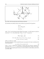
The idea consists in determining the minimum and maximum differences hmin (ϕ ) , hmax (ϕ )

s

s

of the point [0, j0] from the set P(s0,q) in the complex plane in some direction ϕ, ϕ ∈ [0, π ] ,

respectively (see Fig. 1).
REMARK 1 It is worth noting that the difference is measured from the point [0, j0] in the
direction ϕ, ϕ ∈ [0, π ] . It means that the difference can be negative (in such a case the
difference is measured from the point [0, j0] in the direction π +ϕ).

s

0
cIm (q)

s0
hmax(ϕ )

s0 ,ϕ
pmax

s0 ,ϕ
pmin

P(s0, q)

s0
ϕ
hmin ( )

pϕ

ϕ
s

0
cRe (q )

[0,j0]

Figure 1. Minimum and maximum distance of P(s0,q) from [0, j0] in a direction ϕ
It can be easily shown that finding the minimum and maximum differences is equivalent to
s
finding the minimum and maximum value of the function cϕ0 (q ) ,

s0
s0
s0

⎡ s0
⎤ ⎣
cφs0 ( q ) = cRe ( q ) cos (φ ) + cIm ( q ) sin (φ ) = ⎣ cRe ( q ) , cIm ( q ) ⎦ . ⎡ cos (φ ) ,sin (φ ) ⎦
⎤

T

(8)

over the set Q.

s
s
From (8) it follows that cϕ0 (q ) is a real quadratic function of q. It means that cϕ0 (q ) is
s0
s0
bounded and hmin (ϕ ) , hmax (ϕ ) are both finite.

The problem of finding extreme values of

s
cϕ0 (q ) on a box Q is a task of mathematical

programming. General formulation of a task of mathematical programming is as follows.
Let us consider the problem of minimization of a function f0(x), where the constraints are
given in the form of inequalities

{

min f 0 (x ) f j ( x ) ≤ b j , j = 1,…, m

}

(9)


116

Systems, Structure and Control

DEFINITION 7 Let a point 0x satisfy all constraints of (9). Let J(0x) be the set of indices, for
which the corresponding constraints are active (i.e., inequality changes to equality):

( ) { ( x) = b }

J 0x = j f j

0

(10)

j

The point 0x is said to be a regular point of the set X given by constraints in (9) if the
gradients ∇f j ( 0 x ) are linearly independent for all j∈J(0x).
Necessary conditions for the extreme values can be formulated by the following theorem.
THEOREM 2 (Kuhn-Tucker conditions (Kuhn & Tucker, 1951))
Let *x be a regular point of a set X and a function f0(x) has in some neighbourhood of *x
continuous first partial derivatives. If the function f0(x) has in the point *x the local minimum
on X, then there exists a (Lagrange) vector *λ∈ℜm such that

m

∇f 0 ( * x ) + ∑ *λr ∇f r ( * x ) = 0
r =1

(11)

λ j ( f j (* x ) − b j ) = 0

*

λ*j ≥ 0
hold for all j = 1,...,m.
REMARK 2 For maximization of a function f0(x) the last inequality of (11) is replaced by
*
λj ≤ 0 .
To apply Theorem 2 for solving the problem it is necessary to check whether the
s
preconditions of this theorem are satisfied. As cϕ0 (q ) is a quadratic function, its first partial
derivatives are continuous ∀q∈Q and the second assumption is satisfied. In our case
s
( q ) = cϕ ( q )
j+1
f j ( q ) = ( −1) qi ,

f

0

0

i = 1,… , l , j = 2 i - 1 , 2 i

(12)

−
i

b j = −q for j even
b j = qi+

for j odd

Then
∇f j ( q ) = ( −1 )
i=

j +1

e( i ) , q ∈ Q , j = 1,… , 2 l ,

(13)

j+1
j
for j odd, i =
for j even
2
2

where e(i) = [0,...,0,1,0,...,0]T with 1 being on the i-th position. Because for any q∈Q only even
or only odd constraints (or none of them) can be active ( qi− < qi+ ) ∀i = 1,…, l , the gradients

∇f j (q ) are linearly independent ∀q∈Q, j∈J(q). It means that all points q∈Q are regular.

s
Due to Theorem 2 it is necessary to determine the gradient ∇cϕ0 (q ) . From (8)
s0
⎡ s0
⎤ ⎡
∇cφs0 ( q ) = ⎣∇cRe ( q) , ∇cIm ( q ) ⎦ . ⎣ cos (φ ) ,sin (φ ) ⎦
⎤

T

(14)


117

Stability Analysis of Polynomials with Polynomic Uncertainty

The components of ∇c k (q ) ,

⎡ ∂c (q )
∂c (q ) ⎤
∇ck (q ) = ⎢ k
,…, k ⎥
∂ql ⎦
⎣ ∂q1

T

(15)

follow from (5):
l
∂c k (q )
(
(
(
= 2biik ) qi + ∑ (birk ) + brik ) ) q r , k = 0,…, n i = 1,… ,l
∂qi
r =1

(16)

r ≠i

From (7)
s0
∇c Re (q ) =

n

∑ ∇c (q ) s
k

k
0

cos(kψ 0 )

k =0

s0
∇c Im (q ) =

n

∑ ∇c (q ) s
k

k
0

(17)

sin (kψ 0 )

k =0

After substituting (12), (13), (14), (15), (16) and (17) to (11) the following system of equations
and inequalities is obtained:

⎡W11
⎢
⎢
⎢
⎢

⎣Wl 1

W1l

Wll

⎡ q1 ⎤
⎢ ⎥
1 −1 0
⎤ ⎢ ⎥ ⎡ w1 ⎤
⎥⎢q ⎥ ⎢ ⎥
0 0 1 −1
⎥.⎢ l ⎥ = ⎢ ⎥
⎥ ⎢ λ1 ⎥ ⎢ ⎥
⎥
⎢ ⎥
0
0 1 − 1⎦ ⎢ ⎥ ⎣ wl ⎦
⎢ ⎥
⎣ λ2 l ⎦

(

)
)= 0
)= 0
)= 0

(18)

λ1 q1 − q1+ = 0

(

λ2 − q1 −

(

q1−

+
λ3 q 2 − q 2

(

−
λ4 − q 2 − q 2

(

(19)

)
)= 0

λ2l −1 ql − ql+ = 0

(

λ2 l − ql −

ql−

λ1 ,…, λ2l ≥ 0 for minimization
λ1 ,…, λ2l ≤ 0 for maximization

(6.1)


118

Systems, Structure and Control

where
k
k
⎤
⎤
⎡ n (
⎡ n (
(
(
Wuv = ⎢∑ (buvk ) + bvuk ) ). s 0 cos(kψ 0 )⎥ . cos(ϕ ) + ⎢ ∑ (buvk ) + bvuk ) ). s 0 sin (kψ 0 )⎥ . sin (ϕ )
⎦
⎦
⎣ k =0
⎣ k =0
k
k
⎡ n

⎤
⎡ n
⎤
wu = ⎢∑ d u( k ) . s 0 cos(kψ 0 )⎥ . cos(ϕ ) + ⎢ ∑ d u( k ) . s 0 sin (kψ 0 )⎥ . sin (ϕ )
⎣ k =0
⎦
⎣ k =0
⎦
u, v = 1,…, l.

The important fact is that the equation (18) is linear. The computational way of solving the
system (18-19) runs as follows. First all the solutions of (19) are determined. This
corresponds to determining of all the parts of the box Q – interior and all the parts of the
boundary of Q (all manifolds with the dimension i, i = 0,..., l-1 containing only points on the
boundary of Q). Each solution of (19) corresponds to 2l linear equations (from (19) it follows
that at least one of λ2i-1, λ2i, i = 1,..., l has to equal zero; if λ2i-1 = 0 then either λ2i = 0 or qi = - qi-,
if λ2i = 0 then either λ2i-1 = 0 or qi = qi+ i = 1,..., l). These 2l equations together with l equations
of (18) form 3l linearly independent linear equations for 3l unknown variables. It means that
there exists a unique solution (*λ,*q) (for each solution of (19)) of system (18-19). Denote by
Tmin (Tmax) the set of t for which these conditions are satisfied,

Tmin = { t:* q ( t ) ∈ Q ,*λ(jt ) ≥ 0 ∀j = 1,...,2l }

Tmax = { t:* q ( t ) ∈ Q ,*λ(jt ) ≤ 0 ∀j = 1,...,2l }

(20)

Then

[ ( )]

(ϕ ) = max [c ( q )]

s0
s
hmin (ϕ ) = min cϕ0 * q ( t )
t∈Tmin

s0
hmax

s0 *

t∈Tmax

ϕ

(21)

(t )

The minimum and maximum differences indicate that the set P(s0,q) lies in the complex
s ,ϕ

s0 ,ϕ
0
plane in the space between the lines p min and p max :
s0 ,ϕ
s0
p min : c Im (q ) = −
s0 ,ϕ

s0
p max : c Im (q ) = −

h s0 (ϕ )
1
s0
c Re (q ) + min
tan (ϕ )
sin (ϕ )

(22)

(ϕ )
1
s0
c Re (q ) +
tan (ϕ )
sin (ϕ )
s0
hmax

In order to determine a convex hull overbounding the set P(s0,q), q∈Q, the procedure
described above is performed for a set of ϕ r ∈ Φ ,

⎧ϕ : 0 ≤ ϕ 1 ≤
Φ=⎨ r
⎩ r = 1,…, R

≤ ϕ R −1 ≤ ϕ R ≤ π ,⎫
⎬

⎭

(23)

It means that the system (18-19) is solved for a set of ϕ. The higher the number R is, the
"more tight" convex hull is obtained.
If one wants to determine the convex polygon computationally the set VΦ(s0) of the
intersections of the following lines has to be determined:


119

Stability Analysis of Polynomials with Polynomic Uncertainty
s
VΦ (s 0 ) = { S m0 : m = 1,…,2 R}

s0 ,
s0 ,
Vrs0 = insec( p minϕ r , p minϕ r +1 )
s0 ,
s0 ,ϕ
V Rs0 = insec( p minϕ R , p max 1 )

V

= insec( p

s0
r+R

s0 ,ϕ r
max

,p

s0 ,ϕ r +1
max

s0 ,ϕ
s0 ,
0
V2sR = insec( p max R , p minϕ1 )

(24)

)

r = 1,…, R − 1
where insec(px, py) denotes the intersection of the lines px and py (see Fig. 2).
s0
cIm (q )
s ,ϕ

0
pmax 2

s ,ϕ

0
pmax 4

conv VΦ (s0 )

s ,ϕ

0
pmax 3

V3s0

V2s0

V4s0

V1s0

V5s0

s
V100

P( s0 , q)

s ,ϕ

0
pmax 5

V9s0

V6s0
s0 ,ϕ 4
min

p

V7s0

V8s0
s ,ϕ

0
pmin 2

s ,ϕ

0
pmin 1

s ,ϕ

0
pmin 3

s ,ϕ

0
pmax 1

s ,ϕ

0
pmin 5

s

[0, j 0]

0
cRe (q )

Figure 1. Convex hull VΦ(s0) for R = 5
The coordinates of intersections are given by

(

s0 ,ϕ
s0 ,ϕ
insec ptermm , ptermm+1

)

s0
s0
⎡ hterm (ϕ2 ) sin (ϕ1 ) − hterm (ϕ1 ) sin (ϕ2 ) ⎤
⎢
⎥
sin (ϕ1 − ϕ2 )
⎢
⎥

=⎢ s
s0
0
hterm (ϕ2 ) cos (ϕ1 ) − hterm (ϕ1 ) cos (ϕ2 ) ⎥
⎢
⎥
⎢
⎥
sin (ϕ1 − ϕ2 )
⎣
⎦

T

(25)

where term stands for min or max.
Now the key theorems can be stated.
THEOREM 3 (Convex polygons overbounding the value set)
Denote by conv A the convex hull of a set A. Then

P (s 0 , q ) ⊆ conv V Φ (s 0 )∀s 0 ∈ C

(26)

Using Theorem 1 the Zero exclusion principle gives a necessary condition for stability of a
family of polynomials (4).


120

Systems, Structure and Control

THEOREM 4 (Sufficient robust stability condition)
The family of polynomials (4) of constant degree containing at least one stable polynomial is
robustly stable with respect to S if

0 ∉ conv VΦ (s 0 ) for all s 0 ∈ ∂S

(27)

where ∂S denotes the boundary of S.
The zero exclusion test can be performed in both graphical and computational way.
The latter is recommended as described below because of saving a lot of time.
THEOREM 5
0∉conv VΦ(s0) if and only if there exists at least one ϕ ∈ Φ , such that
s0
s0
s0
s0
hmin (ϕ ) ≥ 0 ∧ hmax (ϕ ) ≥ 0 or hmin (ϕ ) ≤ 0 ∧ hmax (ϕ ) ≤ 0

(28)

Theorem 5 makes it possible to decide about zero exclusion or inclusion without computing
the set of intersections VΦ(s0). Proofs of all three theorems are evident from the construction
of convex polygons and Zero exclusion theorem.
Let us illustrate the described procedure of checking robust stability of quadratic interval
polynomials on two examples. As arbitrary stability region can be chosen a discrete-time
uncertain polynomial will be considered at first.

EXAMPLE 1 Let a family of discrete-time polynomials be given by

P (z , q ) = c2 (q )z 2 + c1 (q )z + c0 (q )
where

q = [q1 , q2 ] , qi ∈ [0,1]
T

and

c 2 (q ) = 1

2
c1 (q ) = 0.2 ⋅ q 2 − 0.5 ⋅ q 2 + 0.1 ⋅ q1 ⋅ q 2

2
c 0 (q ) = −0.3 ⋅ q1 + 0.2 ⋅ q12 − 0.5 ⋅ q 2 + q1 ⋅ q 2

The question is whether this family of polynomials is Schur stable.
jω

In this case the stability region S is the unit circle, therefore its boundary ∂S = e ,
ω ∈ [0,2π ] . The Zero exclusion principle will be tested graphically. Due to symmetry it is
sufficient to plot the value set only for the points

s 0 = e jω , ω ∈[0, π ] . The corresponding

plot of the value sets and their convex hulls is shown in Fig. 3 and Fig. 4 (R = 6) respectively.
As 0∉VΦ(s0) for all s0∈∂S, the polynomial P(z,q) is robustly Schur stable. In Fig. 5 and Fig. 6

the value set and the convex hull for
plotted (R = 4 and R = 14 respectively).

s 0 = e jπ / 3 and different number of angles ϕ r is


Stability Analysis of Polynomials with Polynomic Uncertainty

Figure 2. Plot of the value set for

s 0 = e jω , ω ∈[0, π ]

Figure 3. Plot of the convex hulls of the value set

121


122

Systems, Structure and Control

Figure 4. The value set and the convex hull for

s 0 = e jπ / 3 and R = 4

Figure 5. The value set and the convex hull for

s 0 = e jπ / 3 and R = 14

EXAMPLE 2 Let a family of continuous-time polynomials be given by

P (s, q ) = c3 (q )s 3 + c2 (q )s 2 + c1 (q )s + c0 (q )
where

q = [q1 , q 2 ] , qi ∈ [0,1]
T


Stability Analysis of Polynomials with Polynomic Uncertainty

and

c3 (q ) = 1

2
c2 (q ) = 7.7640 + 6.6486q1 + 7.0064q2 + 9.9945q12 + 7.0357q2 + 5.6677q1 ⋅ q2
2
c1 (q ) = 4.8935 + 3.6537q1 + 9.8271q2 + 9.6164q12 + 4.8496q2 + 8.2301q1 ⋅ q2

2
c0 (q ) = 1.8590 + 1.4004q1 + 8.0664q2 + 0.5886q12 + 1.1461q2 + 6.7395q1 ⋅ q2

The question is whether this family of polynomials is Hurwitz stable.

Figure 7. Plot of the convex hulls of the value sets for s0 = jω, ω∈[0,5]

Figure 8. Plot of the convex hulls of the value sets for s0 = jω, ω∈[0,1]

123

124

Systems, Structure and Control

Figure 9. Plot of the determinant of the matrix H 2 ( q )

∂S = jω ,
ω ∈ [ −∞, ∞] . Due to symmetry it is sufficient to plot the value set only for s0 = jω,
ω ∈ [0, ∞] . The corresponding plot of the convex hulls for ω ∈ [0,5] is shown in Fig. 7. As

Here the stability region S is the imaginary axis, therefore the boundary

from this figure it is not apparent, whether zero is included or not, the same plot for
ω ∈ [0,1] is shown in Fig. 8. From that it is clear that 0∉VΦ(s0) for all s0∈∂S. The polynomial
P(s,q) is robustly Hurwitz stable.
The obtained result can be confirmed by plotting the determinant of the (n-1)-th order
Hurwitz matrix H 2 ( q ) and checking its positivity as c0 (q ) is positive for admissible q

evidently. Fig. 9 confirms the obtained result.

4. Polynomials of general polynomic parameter uncertainty
The result obtained in Theorem 5 is applicable for uncertain polynomials with arbitrary
polynomic parameter dependency as well. In such case it is necessary to determine if the
s
function cϕ0 (q ) is positive or negative on the set Q or it allows both positive and negative
s
values on this set, i.e., if there exists a q1∈Q such that cϕ0 (q 1 ) > 0 and q2∈Q such that

s

s
cϕ0 (q 2 ) < 0 . Since cϕ0 (q ) is a polynomic function its positivity can be tested by effective
algorithm of Bernstein expansion (Garloff, 1993).
The algorithm gives only sufficient stability condition. If for all s0∈∂S at least one ϕ r is
s
determined, such that the function cϕ0 (q ) is only positive or only negative on the set Q,

then the origin is excluded from the convex hulls of value sets for all s0∈∂S and therefore
also from the value set itself and the family of polynomials is stable. If not, it is not possible
to decide about robust stability of the family.


Stability Analysis of Polynomials with Polynomic Uncertainty

125

The main advantage of this algorithm is that the number of coefficients of multivariate
s
polynomic function cϕ0 (q ) is considerably smaller than the of Hurwitz determinant

det( H n −1 (q )) especially for higher number of uncertain parameters (however still moderate)
because using the value set algorithm only the coefficients of tested polynomial are needed
to store. For example, a polynomial of degree n = 5 with l = 4 uncertain parameters with
highest degree equal to 4 appearing in each variable in each original coefficient contains
generally 120 coefficients. The determinant of (n-1)-th order Hurwitz matrix, which has to be
tested for positivity, contains generally 83521 coefficients. If the number of parameters is
doubled (l = 8), the uncertain polynomial contains 240 coefficients, but the determinant of
(n-1)-th order Hurwitz matrix contains huge 6.98⋅109 coefficients which is out of memory for
standard computers. Therefore this algorithm can deal with much larger problems. This is
demonstrated on the benchmark example of Fiat Dedra engine.

The proposed algorithm will be demonstrated on some examples and its efficiency
compared with the of original application of algorithm of Bernstein expansion.
EXAMPLE 3 Let a family of continuous-time polynomials be given by

p (s, q ) = c3 (q )s 3 + c2 (q )s 2 + c1 (q )s + c0 (q )
where

q = [ q1 , q2 , q3 ] , qi ∈ [ 0,1] , i = 1, 2,3
T

and
2
2
2
2 2
2
c 3 ( q ) = q1 + q1 + 3q2 + 1q1 q2 + 5q1 q2 + 2 q1 q2 + q1 q2 + 3q3 + 4q1 q3 + q1 q3 + 3q2 q3
2
2
2
2 2
2
2 2
2
+2 q1 q2 q3 + q1 q2 q3 + 4q2 q3 + 4q1 q2 q 3 + 4q1 q2 q3 + 3q1 q 3 + 2 q1 q3 + 3q2 q3
2
2
2
2 2
2 2

2 2 2
+5q1 q 2 q 3 + 3q1 q2 q3 + 2 q2 q3 + 4q1 q 2 q3 + 4q1 q 2 q3 ;
2
2
2
2 2
2
c 2 ( q ) = 8 + 3q1 + 3q1 + 3q 2 + 5q1 q2 + 2 q1 q2 + 10q2 + 3q1 q2 + 8q1 q2 + 9q3 + 3q1 q3
2
2
2
2 2
2
2
+ q1 q3 + 3q 2 q 3 + 7 q1 q2 q3 + 5q2 q 3 + 6q1 q2 q 3 + 7 q1 q2 q 3 + 6q3 + 7 q1 q 3
2 2
2
2
2
2
2 2
2 2
2 2 2
+8q1 q3 + 9q2 q3 + 10q1 q2 q3 + 9q1 q 2 q 3 + 2 q 2 q3 + 10q1 q 2 q3 + 9q1 q2 q 3 ;

2
2
2
2 2
2

c 1 ( q ) = 6 + 7 q1 + q1 + 8q 2 + 5q1 q2 + 9q1 q 2 + q1 q2 + 7 q1 q2 + 6q3 + 9q1 q 3 + 5q1 q3
2
2
2
2 2
2
2
+5q2 q3 + 4q1 q2 q 3 + 4q1 q2 q 3 + 4q 2 q3 + 9q1 q2 q 3 + 8q1 q2 q 3 + 9q3 + 8q1 q3
2 2
2
2
2
2
2 2
2 2 2
+9q1 q3 + 8q2 q3 + 4q1 q 2 q3 + 4q1 q2 q3 + 2 q2 q3 + 4q1 q2 q3 ;
2
2
2
2
2
c 0 ( q ) = 6 + q 1 + q 1 + 6 q 2 + 9 q 1 q 2 + 4 q 1 q 2 + 7 q 2 + q 1 q 2 + 5q 3 + 9 q 1 q 3 + 8q 1 q 3
2
2
2
2 2
2
+8q2 q3 + 2 q1 q2 q 3 + 7 q1 q2 q3 + 2 q2 q3 + 8q3 + q1 q2 q3 + 2 q1 q2 q3 + 2 q3
2
2 2

2
2
2
2
2 2
2 2
2 2 2
+5q1 q3 + q1 q3 + 6q2 q3 + 2 q1 q2 q3 + 9q1 q2 q3 + 3q2 q3 + 5q1 q2 q3 + 8q1 q2 q3

The dependency of polynomial coefficients c j (q), j = 0,… , 3 is no longer quadratic and
Bernstein algorithm will be used to check positivity or negativity of all the distances. The
algorithm checks in 0.34 seconds that for ω∈[0,2] with step 0.01 (R=10) the origin is excluded


126

Systems, Structure and Control

from all the convex hulls of value sets and therefore also from the value set itself and the
family of polynomials is stable. This result is also confirmed by plotting the value set (Fig.
10). The Bernstein algorithm (Zettler & Garloff, 1998) applied on value sets gives the same
result in 0.94s. The algorithm of Bernstein expansion can be also employed on positivity test
of Hurwitz determinant. Using symbolic computations for determination of determinant of
Hurwitz matrix the Bernstein algorithm reports the same result after 3.54s.

Figure 10. Plot of the value sets of P ( s, q) for ω ∈ [0,1.5]

5. Fiat-Dedra engine
Let us consider a model of the Fiat Dedra engine given in (Barmish, 1994). The focal point is
the idle speed control problem, which is particularly important for city driving; that is, fuel

economy depends strongly on engine performance when idling.
The model has 7 uncertain parameters and a design of a fixed output controller leads to
characteristic polynomial of 7-th order,
7

p ( s, q ) = ∑ a j (q ) s j

(29)

j =0

The coefficients a j (q ) , j = 0,…,7 being polynomic functions of the parameters qi, i = 1,...,7
are listed in (Barmish, 1994).
The parameters and the frequency are supposed to vary inside the following intervals:

q1 ∈ [2.1608, 3.4329]; q2 ∈ [0.1027, 0.1627]; q3 ∈ [0.0357, 0.1139];
q4 ∈ [0.2539, 0.5607]; q5 ∈ [0.0100, 0.0208]; q6 ∈ [2.0247, 4.4962];
q7 ∈ [1.0000, 10.000]; ω ∈ [0.0000, 2.3410]

(30)


Stability Analysis of Polynomials with Polynomic Uncertainty

127

The question is whether the uncertain polynomial (29) is robustly stable for the parameters
and frequency given in (30).
Firstly it has to be noted that this problem is relatively large and it is not possible to
compute the determinant of the 6-th order Hurwitz matrix because storage capacity of a

standard computer is too low to store all its coefficients.
The frequency step was chosen 0.01, the sufficient number of direction angles was 10. The
described algorithm reports in 5.53s that the characteristic polynomial (29) is stable that
corresponds to the result obtained by the Bernstein expansion (Zettler and Garloff, 1998) in
7.48s. All the computations were performed on a Pentium 4 CPU 3GHz 504MB RAM.

7. Conclusion
The algorithm checking robust stability of polynomials with polynomic dependency of its
coefficients on vector interval parameter was presented. The method is based on testing the
value set in frequency domain. The value set evaluated in a point lying on the boundary of
stability region is overbounded by a convex polygon. The zero exclusion test is performed
by positivity checking of multivariate polynomic functions using the Bernstein algorithm.
The procedure results in sufficient stability condition. The main advantage of the presented
algorithm over those based on computation of Hurwitz determinant consists in its capability
of treating relatively large problems because of the low requirements on computer storage
capacity. Moreover, arbitrary stability region can be chosen. Efficiency of the algorithm was
verified on the benchmark example of the Fiat Dedra engine control by comparison with the
Bernstein expansion algorithm.

8. Acknowledgements
This work has been supported by the project INGO 1P2007LA297, Research Program
MSM6840770038 (sponsored by the Ministry of Education of the Czech Republic) and the
project 1H-PK/22 (sponsored by Ministry of Industry and Trade of the Czech Republic).

9. References
Ackermann, J. (1993). Robust Control, Systems with Uncertain Physical Parameters, Springer,
ISBN 0-387-19843-1, London
Barmish, B.R. (1994). New Tools for Robustness of Linear Systems. Macmillan Publishing
Company, ISBN 0-02-306005-7, New York
Bartlett, A.C., Hollot, C.V. & Lin, H. (1988). Root Location of an Entire Polytope of

Polynomials: It suffices to check the edges, Mathematics of Controls, Signals and
Systems, Vol. 1, No. 1, pp. 61-71, ISSN 0932-4194
Bhattacharyya, S. P., Chapellat, H. & Keel, L. H. (1995). Robust Control: the Parametric
Approach, Prentice-Hall Inc, ISBN 978-0137815760, New York
Garloff, J. (1985). Convergent Bounds for the Range of Multivariate Polynomials. Interval
Mathematics, Lecture Notes in Computer Science, K. Nickel (Ed.), pp. 37-56, Springer
Verlag, ISBN:3-387-16437-5, Berlin
Garloff, J. (1993). The Bernstein algorithm. Interval Computations, Vol. 2, No. 6, pp. 154-168,
ISSN 0135-4868


128

Systems, Structure and Control

Garloff, J., Graf, B. & Zettler, M. (1997). Speeding Up an Algorithm for Checking Robust
Stability of Polynomials. Fachhochschule Konstanz, Internal Report
Gaston de, R.R. & Safonov, M.G. (1988). Exact Calculation of the Multiloop Stability Margin.
IEEE Transactions on Automatic Control, Vol. 33, No. 2, pp. 156-171, ISSN 0018-9286
Chen, X. & Zhou, K. (2003). Fast parallel-frequency-sweeping algorithms for robust Dstability, IEEE Transactions on Circuits and Systems, Vol. 50, No. 3, pp. 418-428, ISSN
057-7122
Kaesbauer, D. (1993). On Robust Stability of Polynomials with Polynomial Parameter
Dependency: Two/three parameter cases, Automatica, Vol. 29., No. 1, pp. 215-217,
ISSN 0005-1098
Kharitonov, V. L. (1978). Asymptotic stability of an equilibrium position of a family of
systems of linear differential equations. Differencialnyje Uravnenija, Vol. 14, No. 11,
pp. 2086-2088, ISSN 0374 0641
Kuhn, H. W. & Tucker, A. (1951). Nonlinear Programming, Proceedings of the 2nd Berkeley
Symposium on Mathematical Statistics and Probability, University of California Press,
Berkeley

Malan, S., Milanese M. & Taragna, M. (1997). Robust Analysis and Design of Control
Systems Using Interval Arithmetics, Automatica, Vol. 33, No. 7, pp. 1363-1372, ISSN
0005-1098
Murdock, T.M., Schmitendorf, W.E. & Forrest, S. (1991). Use of a Genetic Algorithm to
Analyze Robust Stability Problems, Proceedings of American Control Conference, pp.
886-889, Boston, MA
Neimark,Y. I. (1949). Stability of Linearized Systems, Aeronautical Engineering Academy,
Leningrad, USSR
Sideris, A. & de Gaston, R.R. (1986). Multivariable Stability Margin Calculation with
Uncertain Correlated Parameters, Proceedings of IEEE Conference on. Decision and
Control, Athens, Greece
Sideris, A. & Sánchez Peňa, R.S. (1989). Fast Computation of the Multivariate Stability
Margin for Real Interrelated Uncertain Parameters, IEEE Transactions on Automatic
Control, Vol. 34., No. 12, pp. 1272-1276, ISSN 0018-9286
Siljak, D. D. (1969). Nonlinear Systems, Wiley, New York
Siljak, D. D. and Stipanovic, D. M. (1999). Robust D-stability via positivity, Automatica, Vol.
35, No. 8, pp. 1477-1484, ISSN 0005-1098
Vicino, A., Tesi, A. & Milanese, M. (1990). Computation of Nonconservative Stability
Perturbation Bounds for Systems with Nonlinearly Correlated Uncertainties, IEEE
Transactions on Automatic Control, Vol. 35., No. 7, pp. 835-841, ISSN 0018-9286
Walter, E. and Jaulin, L. (1994). Guaranteed Characterization of Stability Domains Via Set
Inversion, IEEE Transactions on Automatic Control, Vol. 39, No. 4, pp. 886-889, ISSN
0018-9286
Zadeh, L. A. and Desoer, C. A. (1963). Linear Systems Theory, McGraw Hill Book Co., New
York
Zettler, M. and Garloff, J. (1998). Robustness Analysis of Polynomials with Polynomial
Parameter Dependency Using Bernstein Expansion, IEEE Transactions on Automatic
Control, Vol. 43, No. 3, pp. 425-431, ISSN 0018-9286

6
Fouling Detection Based on Parameter
Estimation
Jaidilson Jó da Silva, Antonio Marcus Nogueira Lima
and José Sérgio da Rocha Neto
Federal University of Campina Grande
Brazil

1. Introduction
A severe problem that may occur when fluids are transported in duct systems and pipelines
is the slow accumulation of organic or inorganic substances along the inner surface over
time. Such accumulation of unwanted material is denoted fouling, and occasionally appears
simultaneously with tube corrosion. Both, fouling and corrosion are major concerns for
plant operation and lifetime in chemical, petroleum, food and pharmaceutical industries,
due to the detrimental impact of such phenomenon on the reliability and security (Rose,
1995), (Cam et al., 2002), (Hay & Rose, 2003), (Siqueira et al., 2004). Tube corrosion is related
to the presence of chemically aggressive trace elements and compounds in the transported
materials, usually attributed to presence of sulfur or halogens. A sketch of the two
occasionally simultaneously appearing processes is illustrated in Fig. 1, where the corrosion
related shrinking of wall thickness is related to the growing fouling layer.

Figure 1. Cross-section view of tube aging processes: inhomogeneous fouling layer (a),
corrosion (b), corrosion and fouling (c)
An example of tube fouling, observed in a selected duct section of an oil refining plant, is
presented in Fig. 2. This duct is under test at the LIEC (Electronic Instrumentation and
Control Laboratory) of Federal University of Campina Grande (UFCG).


130

Systems, Structure and Control

The deposition rate commonly is very low, and it may take several months until critical
thickness values are reached. Fouling in chemical plant duct systems and pipelines accounts
for severe problems in plant operation as: reduction of the internal diameter of the tube;
reduction of mechanical integrity and strength, reduction of plant operation lifetime,
increase of the applied pressure to maintain flow through-put, crack formation and possibly
catastrophic break-up. The associated increase of the energy consumption also comes along
with higher operation and maintenance costs.

Figure 2. Photography showing the fouling layer formed in a duct section that transports
crude oil (Petrobras-BR)
Duct systems and pipelines thus require regular and periodic inspection. Several methods
have been proposed for early fouling detection in ducts, based on mass flow reduction
(Krisher, 2003), electric resistance (Panchal, 1997) and ultrasonic techniques (Silva et al.,
2005), (Lohr & Rose, 2002).
The key idea of the mass flow reduction technique is to monitor the corrosion process of a
plate, made of the same material as the ducts. Such plate is put inside the pipe to obtain
information regarding the fouling process (Krisher, 2003). The second group of methods,
named electric resistance sensor techniques, is based on the analysis of the sensor resistance
value to identify modifications in the pipe inner surface (Panchal, 1997). These two methods
are intrusive, i.e. the elements for monitoring must be put inside the pipeline. This is a
disadvantage, since plant operation should be interrupted for installation and analysis of the
elements. On the other hand, the methods based on ultrasound are advantageous over those
aforementioned methods, since those methods are not intrusive (Silva et al., 2005).


Fouling Detection Based on Parameter Estimation

131

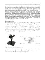
Guided acoustic waves are generated by the interference of Longitudinal (L) and Transverse
(T) wave types: The longitudinal wave is generated when the movement of the particles is
parallel to the wave propagation direction. The transverse wave is generated when the
movement of the particles is perpendicular to the wave propagation direction. Guided
waves are generated by the interference of these two wave types, when the thickness of the
wall under test is smaller or equal than the wavelength of wave (Rose, 1995), (Lohr & Rose,
2002). Fig. 3 shows the formation of guided waves in a plate, when the thickness (d) of the
plate is smaller or equal to the wavelength of wave (λ) (Silva et al., 2007).

Figure 3. Representation of guided acoustic waves
Thus, to generate guided waves, two basic conditions are necessary: First, the pipe wall
thickness under test should be smaller or equal than the wavelength of the spread signal,
and this is possible adjusting the excitation frequency of the pulser; second, the angles of the
used transducers must be chosen adequately. The angles of the transducers are determined
by the shape of the wedge couplers that are made of acrylic. In the present case, it was
observed that for angles larger than 40 deg the guided waves were not generated and the
receiver didn't detect the transmitted signal (Silva, 2005). The transmitted waves were
detected for wedge angles of 30 deg and 40 deg (commercial angular transducers are usually
provided for 30 deg, 40 deg and 45 deg angles) (Silva, 2005).
Guided waves can travel up to 200 m, but there is a reduction in the amplitude of the signal
due the attenuation in the medium and the distance (Rose, 1995). For the studied pipe, tests
were accomplished with a distance variation among the transducers from 5 to 70 cm (size of
the removable part of the pipe) and no amplitude reduction was observed, without fouling.
The ultrasonic transducers are typically excited with pulses and amplitudes that vary
between 100 and 1000 V. The received signal can vary from microvolts to some volts. The
received signal may exhibit frequency characteristics very different from the pulses used to
excite the transmitter transducer, due the characteristics of the propagation media
(Fortunko, 1991).

132

Systems, Structure and Control

After recording at the receiver, the signals are amplified and filtered. The parameters like
gain and bandwidth of the receiver are adjusted in agreement with the characteristics of the
system under test. Choice of gain and bandwidth are also influenced by the used
transducer, discontinuities and characteristics of the frequency response of the pulser. When
the ultrasonic signal encounters a new interface (different material), the signal spreads also
into this interface, and modifies the characteristics of the transmitted signal.
This chapter presents the use of a model for ultrasonic pulses, which spread through guided
waves in a pipe, for fouling detection. The main goal is to estimate the parameters of the
model and to observe the variations of these parameters with the presence of the fouling.
This chapter is organized in six sections: the first part is the introduction; section 2, the
models and estimation method for ultrasonic pulses, in section 3 the proposed system, in
section 4 the simulation results, experimental results in section 5 and concluding remarks
are outlined in section 6.

2. Models and estimation for ultrasonic pulses
Some models of ultrasonic pulses are based on the diffraction scalar theory, while piezoelectric transducers were employed (Calmon et al, 2000).
When an ultrasonic pulse spreads through a layer of a medium of different material, the
waveform of the pulse is modified, due to the attenuation and dispersion. In many media, a
characteristic attenuation, which increases with frequency, has been observed. As result, the
high frequency components of the pulse are more attenuated than the low frequency
components. After crossing the layer, the transmitted pulse differs from the incident pulse,
and it presents a different form (amplitude, frequency, phase) (He, 1998).
The patterns of ultrasonic pulses present important information regarding form, size and
orientation of the reflections, as well as, the micro-structure of the propagation media of the
pulses (Dermile & Saniie, 2001a), (Dermile & Saniie, 2001b).

Models of parametric signals are used to analyze ultrasonic pulses. These models are
sensitive to the characteristics of the signal as bandwidth factor, return time, central
frequency, amplitude and phase of the ultrasonic pulse. Some advantages have been
discovered using signal modeling. First, estimates of parameters with high resolution can be
found; second, the accuracy of the estimation can be evaluated; third, the analytical
relationships between the parameters of the model and physical parameters of the system
can be established. The ultrasonic pulses can be modeled in terms of Gaussian pulses,
affected by noise. Each Gaussian pulse in the model is a non-linear function of the following
parameters: bandwidth (α), return time (τ), central frequency (fc), amplitude (β) and phase
(φ). The estimation of these parameters can be obtained by non-linear parameter estimation
techniques (Dermile & Saniie, 2001a), (Dermile & Saniie, 2001b).
Equation (1) is used by Dermile & Saniie (Dermile & Saniie, 2001a), (Dermile & Saniie,
2001b) to model the ultrasonic pulses.
2

S (θ , t ) = β e −α ( t −τ ) cos(2πfc(t − τ ) + ϕ )

(1)

Where θ = [α τ fc β φ] represents the parameters to be estimated. The bandwidth determines
the pulse time duration in the time domain, the return time is related with the location of the
reflecting surface, the central frequency is governed by the frequency of the displacements