Systems, Structure and Control 2012 Part 8 potx

Fouling Detection Based on Parameter Estimation

133
in the material. The pulse displays an amplitude and a phase, according to the impedance,
size and orientation of the reflecting surface. This model is used for parameter estimation, in
combination with tests that use the pulse-echo method, and a transducer that operates as
both, a pulser and receiver.
Considering the effect of the noise in the estimation, a noise process can be included to the
model (Dermile & Saniie, 2001a), (Dermile & Saniie, 2001b). Thus, the ultrasonic pulse can be
modeled by equation (2):

() ( ,) ()
x
tStet
θ
=+

(2)

Where S(θ,t) denotes the model of the ultrasonic pulse and e(t) denotes the additive white
Gaussian noise.
This model can be extended to consider multiple ultrasonic pulses by equation (3):

1
() ( ,) ()
M
m
m
yt S t et
θ
=

=+
∑

(3)

Each parametric vector θ
m
defines the form and location of the corresponding pulse
completely. For computer programming purposes, the observation model expressed by
equation (2) for an ultrasonic pulse can be written in the discrete form (Dermile & Saniie,
2001a), (Dermile & Saniie, 2001b), (Silva et al., 2007).
The Gaussian pulse model has been chosen as the algorithm for parameter estimation, since
this model is more accurate and the parameters resemble the ultrasonic pulse in a more
complete approach. The Gaussian pulse model is thus appropriate to determine the
parameters of the guided waves method and the analysis of the fouling process is achieved
by observing the variation of the estimated parameters.
The estimation problem relies on the determination of the parameters of the model, and
modifications of these parameters in presence of fouling. Here, the non-linear estimation
approach is employed, using programs developed with the MATLAB code (Hansenlman &
Littlefield, 1996).
3. Proposed system
The proposed system for fouling monitoring using ultrasonic transducers is illustrated by
the block diagram presented in Fig. 4. This system is composed by the ultrasonic pulser and
receiver which are connected to the transducers and coupled to the pipe, in order to
generate longitudinal guided waves.
Systems, Structure and Control

134

Figure 4. Block diagram of the proposed system with the pulser and receiver

The block diagram of the pulser circuit is shown in Fig. 5. The diagram comprises basically a
DC power supply and a pulse wave generator, used to activate an analog switch, to obtain
the pulses with the amplitude and frequency necessary to excite the ultrasonic transducer. A
current drive is used to supply the current required by the analog switch.

Figure 5. Block diagram of the pulser circuit
The waveform of the pulser output signal is shown in Fig. 6. This signal has 80 V maximum
amplitude and 500 kHz frequency. These values are necessary for generation of the guided
waves and monitoring at the receiver.
Fouling Detection Based on Parameter Estimation

135

Figure 6. Waveform of the pulser output signal
The excitement signal of the pulser is a train of pulses with 80 V amplitude and 500 kHz
frequency. This amplitude guarantees a minimum level of received signal (in the mV range),
for smaller amplitude the received signal is too low to excite the receiver transducer. This
frequency is necessary to guarantee the generation of the guided waves, once the
propagation speed in the galvanized iron is known (4600 m/s) and the wavelength should
be larger or equal than the pipe wall thickness (2.0 mm) (Silva et al., 2005).
A simplified block diagram of the receiver is presented in Fig. 7. In this diagram an initial
amplification stage is used to increase the amplitude of the received signal, and a narrow
band RF-filter to select the monitored signals.



Figure 7. Simplified block diagram of the receiver
The receiver is designed, using amplification and filtering stages to detect the signals from
the receiving transducer. The receiver circuit utilizes the integrated circuit AD8307, which is
a logarithmic amplifier. Its output is a voltage value, proportional to the logarithm of the

input signal amplitude, and its input impedance is equal to 50 Ω.
Systems, Structure and Control

136
The waveform of the receiver output signal is presented in Fig. 8. This signal has 100 mV
maximum amplitude and frequency in the MHz range, representing the typical feature of
ultrasonic signals.

Figure 8. Waveform of the receiver output signal
The signals are monitored, using a digital oscilloscope. To detect the fouling layer, initially
the amplitude reduction of the signals has been considered. However, towards an accurate
analysis, other relevant features of the received signals are required as: frequency variations
and phase. As mentioned before, the goal is to determine the parameters of a model for
ultrasonic pulses and to analyze the variations of these parameters, under the effect of the
fouling in the system. The fouling process was emulated by means of an experimental
platform, in which the temperature, pressure and flow are monitored and controlled. Before
each experiment, the tube was taken out of the experimental platform and the accelerated
fouling layer deposition process inside the tube initiated. To speed up the fouling process,
the same substances related to actual petroleum exploration were mixed with water and put
into the pipe. The proportions of the substances deposited in the tube were subsequently
increased. For 100 l of water, the following concentrations were used: 24.05 g of Ca(OH)
2
; 9.9
g of MgSO
4
; 2.472 kg of NaCl; and 16.99 g of BaSO
4
. These proportions are the same, as
found in the petroleum treatment factory of Petrobras in Guamare-RN-Brazil.
As outlined before, the model is used to determine the parameters using the method of the

guided waves and the variation of the estimated parameters in the model of Gaussian
pulses.
A diagram of the experimental platform for data acquisition is shown in Fig. 9. This
platform was developed, in which the temperature, pressure and flow are monitored and
Fouling Detection Based on Parameter Estimation

137
controlled (Silva, 2005). The tubes were used as a medium to guide ultrasonic waves and
periodically over several weeks measurements were performed to monitor the fouling
process (Silva et al., 2007).

Figure 9. Diagram of the experimental platform
With the acquired data and using the models, the estimated parameters of the system have
been used to analyze the behavior of the ultrasound signal and to observe the influence of
the fouling. The non-linear estimation methods (least square non-linear) were used, with the
software MATLAB, to determine the model parameters (Hansenlman & Littlefield, 1996).
4. Simulation results
A preliminary simulation study was accomplished by using the model for ultrasonic pulses
provided in (1). The single pulse case was simulated and the parameter vector θ was
estimated, using a program developed with MATLAB. In Table 1, the values obtained with
the simulation for a single pulse are shown. The choice of θ
0
, the initial parameter vector, is
quite critical to obtain good results with relatively few iteration steps. The selection of the
initial parameter relies on the characteristics of the observed signal.

Real Parameters Estimated Parameters
α 38.00 36.00
τ 0.70 0.50
f

c
18.00 16.00
β 0.80 0.70
φ 0.90 0.80
Table 1. Simulation results with single pulses
Systems, Structure and Control

138
A signal with multiple pulses was also simulated with a program using MATLAB. In Table
2 are presented the values obtained with the simulation for multiple pulses.

Real Parameters Estimated Parameters
α
0
38.00 36.00
τ
0
0.70 0.50
f
c0
18.00 16.00
β
0
0.80 0.70
φ
0
0.90 0.80
α
1
38.00 36.00

τ
1
1.50 1.40
fc
1
16.00 14.00
β
1
0.60 0.50
φ
1
0.85 0.80
Table 2. Simulation results with multiple pulses
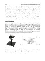
The results of simulation for the parameter estimation of a single pulse are presented in Fig.
10. The estimated parameters curve is quite similar with the real parameters curve. For this
simulation the processing time is 4.42 s, the measurement error is 0.0099 (quadratic medium
error) and the number of iterations is 20. The results of simulation for the parameter
estimation of the signal with multiple pulses are presented in Fig. 11; this simulation also
provides an excellent result in relation to the estimated parameters. For this simulation the
processing time is 215.37 s, the measurement error is 0.0331 and the number of iterations is
40 (Silva et al., 2007).

Figure 10. Results of the simulation for a single pulse: The points represent the real signal
and the full line represents the estimated signal
Fouling Detection Based on Parameter Estimation

139

Figure 11. Results of the simulation for a multiple pulse: The points represent the real signal
and the full line represents the estimated signal

As the number of ultrasonic pulses increases, the dimension of the parameter vector
increases and, consequently the number of iteration steps also increases. To reduce the
number of parameters to be estimated, we have employed spectral analysis (FFT) to
determine what frequencies are present in the signal detected with multiple pulses, using
MATLAB. The results of the simulation of a signal with multiple pulses and the FFT of this
signal are presented in the Figs. 12 and 13 respectively. It was considered as parameters for
the real signal: α
0
= 38, τ
0
= 0.5, f
c0
= 20, β
0
= 0.8, φ
0
= 1; and α
1
= 28, τ
1
= 1.0, f
c1
= 15, β
1
= 0.6,
φ
1
=0.80; and α
2
= 14, τ

2
= 1.5, f
c2
= 10, β
2
= 0.9, φ
2
= 0.90. Using the FFT, the present
frequencies in the signal can be determined accurately, thus reducing the number of
parameters to be estimated. Fig. 13 shows the three present frequencies in the signal of the
Fig. 12 (Silva et al., 2007).
With these simulations, it is possible to observe the behavior of the Gaussian pulses and to
analyze the estimated parameters for these pulses, as well as to test the quality of the
developed programs and to evaluate its performance. An important result in relation to the
estimation procedure is the choice of the initial parameters, which is obtained from an
observation of the measured signals. A bad choice increases the processing time
substantially, and the estimation error.
Systems, Structure and Control

140

Figure 12. Representation of a signal with multiple pulses

Figure 13. Representation of FFT for the signal of the Fig. 12.
Fouling Detection Based on Parameter Estimation

141
5. Experimental results
A calibration step to define the pipeline signature is initially carried out and the pipe is
completely cleaned, ensuring absence of a fouling layer. The inclination angle of the used

transducers is 30
0
. The maximum frequency of operation is 2 MHz, the transmitter is excited
with pulses of 80 V and the sampling frequency is 100 MHz. The received signal is
monitored, and the characteristics of these signals (amplitude, frequency, etc) are taken as
reference for fouling detection.
The new results presented in this section were obtained with the same methodology
presented in Silva (Silva et al., 2007).
In the experimental platform, it was possible to acquire the data in the receiver output by
means of a digital oscilloscope. The obtained ultrasonic signals are illustrated in Figs. 14, 15
and 16, respectively. The signal shown in Fig. 14 represents the pipe signature, i.e., the pipe
without fouling. The signal shown in Fig. 15 presents the pipe with 1 mm of fouling and Fig.
16 depicts an ultrasonic signal related to a pipe exhibiting a 3 mm fouling layer.
For the signal of Fig. 14, the processing time is 145.35 s, the measurement error is 2.65
(quadratic medium error) and the number of iterations is 8. For the signal of the Fig. 15 the
processing time is 38.30 s, the measurement error is 1.25 and the number of iterations is 6.
And for the signal of the Fig. 16 the processing time is 34.25 s, the measurement error is 1.15
and the number of iterations is 4.




Figure 14. Representation of the receiver output signal without fouling using MATLAB
Systems, Structure and Control

142

Figure 15. Representation of the receiver output signal with 1 mm of fouling using MATLAB

Figure 16. Representation of the receiver output signal with 3 mm of fouling using MATLAB

Fouling Detection Based on Parameter Estimation

143
From the analysis of the ultrasonic signal, it was found that the amplitude reduction
provides important information regarding the fouling process. This effect occurs, since the
fouling layer modifies the propagation medium of the ultrasonic signals, thus providing a
second leakage path in the received signal.
A further program, developed with MATLAB was used to determine the spectral features
and frequencies in the measured signals in the time domain from Figs. 14, 15 and 16
respectively. The signals obtained with the FFT are represented in Figs. 17, 18 and 19
respectively. For the first signal, the determined frequency is 29 MHz, for the second signal
(with 1 mm of fouling) the determined frequency is 27 MHz and for the third signal (with 3
mm of fouling) the determined frequency is 24 MHz. The estimated parameters for the
frequency of the three signals represent a good approximation in relation to the measured
real signal.
With the use of FFT, it was possible to determine the frequencies that are present in the
ultrasonic signals. Since the frequencies of the pulses are not needed of being estimated and
the number of parameters is reduced, the estimation times and the iteration numbers are
also reduced.




Figure 17. Representation of FFT for the measured signal without fouling
With the model for Gaussian pulses and using a program developed in MATLAB, it was
possible to identify the parameters for the measured signal that are represented in Figs. 14,
15 and 16. The results with the parameter estimation for these signals are illustrated in Figs.
20, 21 and 22 respectively, and we can observe that the parameter modifications are due the
fouling process in tubes.
Systems, Structure and Control

144

Figure 18. Representation of FFT for the measured signal with 1 mm of fouling


Figure 19. Representation of FFT for the measured signal with 3 mm of fouling
Fouling Detection Based on Parameter Estimation

145

Figure 20. Representation of the measured signal (dashed signal) and of the estimated
(continuous signal) without fouling


Figure 21. Representation of the measured signal (dashed signal) and of the estimated
(continuous signal) with 1 mm of fouling
Systems, Structure and Control

146

Figure 22. Representation of the measured signal (dashed signal) and of the estimated
(continuous signal) with 3 mm of fouling
The estimated parameters for the signals are presented in the Table 3.

Signal
without
fouling
Signal with
1 mm of

fouling
Signal with
3 mm of
fouling
α 85.0 80.0 75.0
τ 0.16 1.95 2.10
f
c
30.0 27.0 24.0
β 0.18 0.14 0.09
φ 0.80 0.85 0.90
Table 3. Estimated parameter values for the measured signal
Analyzing the data in Table 3, we observe that the parameters bandwidth (α), central
frequency (f
c
) and amplitude (β) decrease with the increase of the fouling layer, while the
parameters return time (τ) and phase (φ) increase.
The presented models are considered as a good approach to resemble recorded real signals.
Parameter variations resulting from the presence of tube fouling are well resolved. The
absolute values of the signals are compared and modifications, as increase or reduction, of
the absolute parameter values are easily observable.
6. Concluding remarks
In this chapter, a signal analysis method of ultrasonic signals has been presented and this
method utilizes a parameter estimation algorithm for fouling detection. The model is based
Fouling Detection Based on Parameter Estimation

147
on Gaussian pulses, therefore this model is more complete and the parameter estimation
provides higher accuracy. Results were obtained with simulations and with acquired
experimental data. For treating of a non-linear system, this problem cannot be solved using

optimization algorithms as efficient as the least square method.
Thus, programs were developed with MATLAB for estimation of non-linear systems. With
the use of the Fast Fourier Transform (FFT) algorithm the spectral features i.e. frequencies
present in the ultrasonic signals were resolved. Since the number of parameters is lowered,
also the estimation time and number of required iterations are reduced.
With this approach presence of fouling layers can be easily detected, taking as reference the
estimated parameters of the clean, fouling free tube section. Systematic variations of these
parameters originate from inner tube fouling deposits. Different points of the pipe have
been evaluated to identify their exact positions.
It is anticipated in future investigations to extend the analysis and include the attenuation
rate of the received signal amplitude, in accordance with the amount of substance deposited
onto the inner tube surface, and to verify the variation of the oscillations as a function of the
substance type deposited inside the pipeline. In addition, it is also desired to evaluate other
methods with ultrasonic waves, such as the circumferential guided wave method.
7. References
Calmon, P.; Roy, O. & Benoist, P. (2000). Simulation of Ultrasonic Examination. IEEE
Ultrasonic Symposium. Pp.1265-1269, 2000.
Cam, E.; Lei, M.; Kocaarslan, I. & Taplamacioglu, C. (2002). Defect detection in a cantilever
beam from vibration data. Kirikkale University. Faculty of Engineering, Department
of Electrical and Electronics. Kirikkale, 2002.
Dermile, R. & Saniie, J. (2001a). Model-based estimation of ultrasonics echoes part I:
Analysis and algorithms. IEEE Transactions on ultrasonics, ferroeletrics and frequency
control. 2001.
Dermile, R. & Saniie, J. (2001b). Model-based estimation of ultrasonics echoes part II: Non-
destructive evaluation applications. IEEE Transactions on ultrasonics, ferroeletrics and
frequency control. 2001.
Fortunko, C. M. (1991). Generation and reception of ultrasonic signal. Ultrasonic Testing
Equipment. Nondestructive Testing Handbook. 2 ed. Ultrasonic Testing. Vol. 7. USA.
1991.
Hansenlman, D. & Littlefield, B. (1996). Mastering MATLAB - A comprehensive tutorial and

reference. Prentice Hall. USA, 1996.
Hay, T. R. & Rose, J. L. (2003). Fouling detection in the food industry using ultrasonic
guided waves. Food Control. Elsevier. 2003.
He, P. (1998). Simulation of Ultrasound Pulse Propagation in Loss Media Obeying a
Frequency Power Law. IEEE Trans. on Ultrasonics, Ferroelectrics and Frequency
Control. Vol. 45, No.1, 1998.
Krisher, A. S. (2003). Technical information regarding coupon testing. ASK Associates. St.
Louis, Missouri. November 2003.
Lohr, K. R. & Rose, J .L. (2002). Ultrasonic guided wave and acoustic impact methods for
pipe fouling detection. Journal of food engineering. Elsevier Science, March 2002.
Panchal, C. B. (1997). Fouling mitigation of industrial heat exchange equipment. Bengell
House. New York. 1997.
Systems, Structure and Control

148
Rose, J. L. (1995). Recent advances in guided wave NDE. IEEE Ultrasonic Symposium. Pp.761-
770. 1995.
Silva, J. J. (2005). Development of a platform for fouling detection in pipelines. Master's degree
dissertation (in Portuguese). UFCG, Campina Grande, Brazil. 2005.
Silva, J. J.; Wanzeller, M. G.; Rocha Neto, J. S. & Farias, P. A. (2005). Development of circuits
for excitement and reception in ultrasonic transducers for generation of guided
waves in hollow cylinders for fouling detection. IEEE Instrumentation and
Measurement Technology Conference. Ottawa, Ontario, Canada. 17-19 May 2005.
Silva, J. J.; Lima, A. M. N. & Rocha Neto, J. S. (2007). Fouling detection based on ultrasonic
guided waves and parameter estimation. 3rd IFAC Symposium on System, Structure
and Control - SSSC 2007. Foz do Iguaçu, Brazil, October, 2007.
Siqueira, M. H. S.; Gatts, C. E. N.; Silva, R. R. & Rebello, J. M. A. (2004). The use of ultrasonic
guided waves and wavelets analysis in pipe inspection. Ultrasonic. Elsevier. Vol. 41,
pp. 785-797. 2004.

7
Enhanced Fuzzy Controller for Nonlinear
Systems: Membership-Function-Dependent
Stability Analysis Approach
H.K. Lam and Mohammad Narimani
Division of Engineering, The King’s College London, Strand, London
United Kingdom
1. Introduction
Fuzzy-model-based (FMB) control approach provides a systematic and effective way to
control nonlinear systems. It has been shown by various applications (Lam et al., 1998; Lian
et al., 2006; (b)Tanaka et al., 1998) that FMB control approach performs superior to some
traditional control approaches. Based on the T-S fuzzy model (Sugeno & Kang, 1988; Takagi
& Sugeno, 1985) the system dynamics of the nonlinear can be represented by some local
linear models in the form of linear state-space equations. With the fuzzy logic technique, the
overall system dynamics of the nonlinear plant is a fuzzy combination of the local linear
models. Consequently, the fuzzy model offers a systematic way and general framework to
represent the nonlinear plants in the form of averaged weighted sum of local linear systems.
This particular structure exhibits favourable property to facilitate the system analysis and
control synthesis.
In general, the stability analysis for FMB control systems can be classified into two
categories, i.e., membership function (MF)-independent (Chen et al.,1993; Tanaka & Sugeno,
1992) and MF-dependent (Fang et al., 2006; Feng, 2006; Kim & Lee 2000; Liu & Zhang, 2003a;
Liu & Zhang, 2003b; Tanaka et al., 1998a; Teixeira et al.,2003) stability analysis approaches.
Under the MF-independent stability analysis, the membership functions of both fuzzy
model and fuzzy controller are not considered during stability analysis. The system
stability is guaranteed to be asymptotically stable if there exists a common positive definite
matrix to a set of stability conditions in the form of Lyapunov inequalities (Chen et al.,1993;
Tanaka & Sugeno, 1992). The main advantages under the MF-independent analysis
approach are 1). The membership functions of the fuzzy controller can be designed freely.
Some simple and easy-to-implement membership functions can be employed to realize the

fuzzy controller to lower the implementation cost. 2). The grades of membership functions
of the fuzzy model are not necessarily known which implies parameter uncertainties of the
nonlinear plant are allowed. Consequently, the fuzzy controller exhibits an inherent
robustness property for nonlinear plant subject to parameter uncertainties. However, the
membership function mismatch (both fuzzy model and fuzzy controller do not share the
same membership functions) leads to very conservative stability analysis results.
Furthermore, it can be shown that the fuzzy controller designed based on the stability
conditions in (Chen et al.,1993; Tanaka & Sugeno, 1992) can be replaced by a liner controller.
Systems, Structure and Control

150
Under the MF-dependent stability analysis approach, the membership functions of both
fuzzy model and fuzzy controller are considered. In (Wang et al., 1996), the importance of
the membership functions to the stability analysis was shown. By sharing the same premise
membership functions between fuzzy model and fuzzy controller which leads to perfect
match of membership functions, relaxed stability conditions were achieved. Further relaxed
MF-independent stability conditions were reported (Fang et al., 2006; Feng, 2006; Kim & Lee
2000; Liu & Zhang, 2003a; Liu & Zhang, 2003b; Tanaka et al., 1998a; Teixeira et al.,2003). As
to achieve perfect match of membership functions between fuzzy model and fuzzy
controller which implies the membership functions of the fuzzy model must be known, the
design flexibility and inherent robustness property of the fuzzy controller are lost. In both
MF-independent and dependent stability analysis approaches, the stability conditions can
be represented in the form of linear matrix inequalities (Boyd et al., 1994), some convex
programming techniques (e.g., MATLAB LMI toolbox) can be employed to solve the
solution to the stability conditions numerically and effectively.
It can be seen that fuzzy controller designed based on stability conditions under MF-
dependent or -independent stability analysis approaches offers different favourable and
undesired properties. It is a good idea to get the most out of these two analysis approaches
by combining the advantages and alleviate the disadvantages of them, thus, to widen the
applicability of the FMB control approach. This idea motivates the investigation in this

chapter. In this chapter, MF-dependent stability analysis approach is employed to
investigate the stability of the FMB control systems under the condition of imperfect match
of membership functions. As a result, the design flexibility and inherent robustness of the
fuzzy controller can be retained (due to the imperfect match of the membership functions)
and the stability conditions can be relaxed (due to the MF-dependent stability analysis
approach). In order to strengthen the stabilization ability of the fuzzy controller, fuzzy
feedback gains, which enhance the nonlinearity compensation ability, are introduced. In
order to carry out stability analysis under MF-dependent Lyapunov-based approach,
membership function conditions are proposed to guide the design of the membership
functions. Based on membership function conditions, some free matrices can be introduced
to the stability analysis and relax the stability conditions.
This chapter is organized as follows. In section II, the fuzzy model and the proposed fuzzy
controller are introduced. In section III, system stability of FMB control system is
investigated using Lyapunov’s stability theory under MF-dependent stability analysis
approach. LMI-based stability conditions are derived to aid the design of the fuzzy
controller for the nonlinear plant. In section IV, simulation examples are given to illustrate
the effectiveness of the proposed approach. In section V, a conclusion is drawn.
2. Fuzzy Model and Enhanced Fuzzy Controller
A fuzzy-model-based control system comprising a nonlinear plant represented by a fuzzy
model and an enhanced fuzzy controller connected in a closed loop is considered.
2.1 Fuzzy Model
Let p be the number of fuzzy rules describing the nonlinear plant. The i-th rule is of the
following format:
Enhanced Fuzzy Controller for Nonlinear Systems:
Membership-Function-Dependent Stability Analysis Approach

151
Rule i: IF
))((
1

tf x
is
i
1
M AND … AND
))(( tf x
Ψ
is
i
Ψ
M
THEN
)()()( ttt
ii
uBxAx +=

(1)
where
i
α
M is a fuzzy term of rule i corresponding to the known function ))(( tf x
α
,
α
= 1, 2,
,
Ψ
; i = 1, 2, , p;
Ψ
is a positive integer;

nn
i
×
ℜ∈A and
mn
i
×
ℜ∈B are known constant
system and input matrices respectively;
1
)(
×
ℜ∈
n
tx is the system state vector and
1
)(
×
ℜ∈
m
tu
is the input vector. The system dynamics are described by,

()
)()())(()(
=1
tttwt
ii
p
i

i
uBxAxx +=
∑

(2)
where,
1=))((
1
tw
p
i=
i
x
∑
,
[]
10))(( ∈tw
i
x for all i (3)

()
∑
×××
×××
p
k
i
tftftf
tftftf
tw

kkk
iii
1=
M
2
M
1
M
M
2
M
1
M
))((()))((()))(((
)))((()))((()))(((
=))((
21
21
xxx
xxx
x
Ψ
Ψ
Ψ
Ψ
μμμ
μμμ
"
"
(4)

is a nonlinear function of x(t) and
)))(((
M
tf
i
x
α
α
μ
,
α
= 1, 2, …,
Ψ
, is the grade of membership
corresponding to the fuzzy term of
i
α
M .
2.2. Enhanced Fuzzy Controller
A fuzzy controller with p rules is considered. The j-th rule of the fuzzy controller is defined
as follows.
Rule j: IF ))((
1
tg x is
j
1
N AND … AND ))(( tg x
Ω
is
j

Ω
N
THEN
()
)()()( ttt
j
xxGu = , j = 1, 2, , p (5)
where
j
β
N is a fuzzy term of rule j corresponding to the function ))(( tg x
β
,
β
= 1, 2, ,
Ω
; j =
1, 2, , p;
Ω
is a positive integer;
()
nm
j
t
×
ℜ∈)(xG
is the constant and time-varying feedback
gains of rule j. The time-varying feedback gain is defined as,

()

jk
p
k
kj
tmt GxxG
∑
=
=
1
))(()( (6)
where
nm
jk
×
ℜ∈G are constant feedback gains. The inferred enhanced fuzzy controller is
defined as,

)())(())(()(
11
ttmtmt
jk
p
j=
p
k
kj
xGxxu
∑∑
=
=

(7)
Systems, Structure and Control

152
where

∑
=
p
j=
j
tm
1
1))((x ,
[]
10))(( ∈tm
j
x , j = 1, 2, , p (8)


(
)
∑
×××
×××
=
p
k
j
tgtgtg

tgtgtg
tm
kkk
jjj
=1
N
2
N
1
N
N
2
N
1
N
)))((()))((()))(((
)))((()))((()))(((
))((
21
21
xxx
xxx
x
Ω
Ω
Ω
Ω
μμμ
μμμ
"

"
(9)
is the normalized grade of membership which is a nonlinear function of x(t).
)))(((
N
tg
j
x
β
β
μ
,
j = 1, 2, , p, is the grade of membership corresponding to the fuzzy term
j
β
N .
Remark 1: It should be noted that the proposed enhanced fuzzy controller of (7) is reduced
to the traditional fuzzy controller (Chen et al., 1993; Fang et al., 2006; Feng, 2006; Liu &
Zhang, 2003a; Liu & Zhang, 2003b; Tanaka et al., 1998a; Teixeira et al., 2003; Wang et al.,
1996) when G
jk
= F
j
for all j where
nm
j
×
ℜ∈F are the constant feedback gains.
3. Stability Analysis
In this section, the system stability of fuzzy-model-based control system formed by a

nonlinear plant in the form of (2) and the enhanced fuzzy controller of (7) connected in a
closed loop, is considered. Based on the Lyapunov stability theory, LMI-based stability
conditions are derived to guarantee the asymptotic stability of the fuzzy-model-based
control systems. For brevity, w
i
(x(t)) and m
j
(x(t)) are denoted as w
i
and m
j
respectively. The
property of the membership functions in (3) and (8), i.e.
∑
=
p
i
i
w
1
=
∑
=
p
i
i
m
1
=
∑∑

==
p
i
p
j
ji
mw
11
= 1 is
utilized to facilitate the stability analysis. From (2) and (7), we have,
⎟
⎟
⎠
⎞
⎜
⎜
⎝
⎛
+=
∑∑∑
=
)()()(
11=1
tmmtwt
jk
p
j=
p
k
kjii

p
i
i
xGBxAx



()
)(
1=11
tmmw
jkii
p
i
p
j
p
k
kji
xGBA +=
∑∑∑
==
(10)
As the membership functions of w
i
and m
j
do not match, which is one of the sources of
conservativeness, the MF-dependent stability analysis approach in (Fang et al., 2006; Feng,
2006; Liu & Zhang, 2003a; Liu & Zhang, 2003b; Tanaka et al., 1998a; Teixeira et al., 2003)

cannot be applied. In the following, membership function conditions are proposed to
alleviate the conservativeness of stability analysis due to the imperfect match of
membership functions. To proceed with the stability analysis, the following Lyapunov
function candidate is employed to investigate the fuzzy-model-based control system of (10).

)()()(
T
tttV Pxx= (11)
where
0
T
>ℜ∈=
×nn
PP . From (10) and (11),