Báo cáo hóa học: "Research Article Minimal Nielsen Root Classes and Roots of Liftings" pptx
Bạn đang xem bản rút gọn của tài liệu. Xem và tải ngay bản đầy đủ của tài liệu tại đây (615.21 KB, 16 trang )
Hindawi Publishing Corporation
Fixed Point Theory and Applications
Volume 2009, Article ID 346519, 16 pages
doi:10.1155/2009/346519
Research Article
Minimal Nielsen Root Classes and Roots of Liftings
Marcio Colombo Fenille and Oziride Manzoli Neto
Instituto de Ci
ˆ
encias Matem
´
aticas e de Computac¸
˜
ao, Universidade de S
˜
ao Paulo, Avenida Trabalhador
S
˜
ao-Carlense, 400 Centro Caixa Postal 668, 13560-970 S
˜
ao Carlos, SP, Brazil
Correspondence should be addressed to Marcio Colombo Fenille,
Received 24 April 2009; Accepted 26 May 2009
Recommended by Robert Brown
Given a continuous map f : K → M from a 2-dimensional CW complex into a closed surface, the
Nielsen root number Nf and the minimal number of roots μf of f satisfy Nf ≤ μf.But,
there is a number μ
C
f associated to each Nielsen root class of f, and an important problem
is to know when μfμ
C
fNf. In addition to investigate this problem, we determine a
relationship between μf and μ
f,when
f is a lifting of f through a covering space, and we
find a connection between this problems, with which we answer several questions related to them
when the range of the maps is the projective plane.
Copyright q 2009 M. C. Fenille and O. M. Neto. This is an open access article distributed under
the Creative Commons Attribution License, which permits unrestricted use, distribution, and
reproduction in any medium, provided the original work is properly cited.
1. Introduction
Let f : X → Y be a continuous map between Hausdorff, normal, connected, locally path
connected, and semilocally simply connected spaces, and let a ∈ Y be a given base point. A
root of f at a is a point x ∈ X such that fxa. In root theory we are interested in finding a
lower bound for the number of roots of f at a. We define the minimal number of roots of f at a
to be the number
μ
f, a
min
#ϕ
−1
a
such that ϕ is homotopic to f
. 1.1
When the range Y of f is a manifold, it is easy to prove that this number is independent
of the selected point a ∈ Y,and,from1, Propositions 2.10 and 2.12, μf, a is a finite
number, providing that X is a finite CW complex. So, in this case, there is no ambiguity in
defining the minimal number of roots of f:
μ
f
: μ
f, a
for some a ∈ Y. 1.2
2 Fixed Point Theory and Applications
Definition 1.1. If ϕ : X → Y is a map homotopic to f and a ∈ Y is a point such that μf
#ϕ
−1
a, we say that the pair ϕ, a provides μf or that ϕ, a is a pair providing μf.
According to 2, two roots x
1
, x
2
of f at a are said to be Nielsen rootfequivalent if
there is a path γ : 0, 1 → X starting at x
1
and ending at x
2
such that the loop f ◦ γ in Y
at a is fixed-end-point homotopic to the constant path at a. This relation is easily seen to be
an equivalence relation; the equivalence classes are called Nielsen root classes off at a.Also
a homotopy H between two maps f and f
provides a correspondence between the Nielsen
root classes of f at a and the Nielsen root classes of f
at a. We say that such two classes under
this correspondence are H-related. Following Brooks 2 we have the following definition.
Definition 1.2. A Nielsen root class R of a map f at a is essential if given any homotopy
H : f f
starting at f,andtheclassR is H-related to a root class of f
at a. The number of
essential root classes of f at a is the Nielsen root number of f at a; it is denoted by Nf, a.
The number Nf, a is a homotopy invariant, and it is independent of the selected
point a ∈ Y , provid that Y is a manifold. In this case, there is no danger of ambiguity in denot
it by Nf.
In a similar way as in the previous definition, Gonc¸alves and Aniz in 3 define the
minimal cardinality of Nielsen root classes.
Definition 1.3. Let R be a Nielsen root class of f : X → Y. We define μ
C
f, R to be the
minimal cardinality among all Nielsen root classes R
, of a map f
, H-related to R,forH
being a homotopy starting at f and ending at f
:
Again in 3 was proved that if Y is a manifold, then the number μ
C
f, R is
independent of the Nielsen root class of f : X → Y . Then, in this case, there is no danger of
ambiguity in defining the minimal cardinality of Nielsen root classes of f
μ
C
f
: μ
C
R
for some Nielsen rootclass R. 1.3
An important problem is to know when it is possible to deform a map f to some
map f
with the property that all its Nielsen root classes have minimal cardinality. When
the range Y of f is a manifold, this question can be summarized in the following: when
μfμ
C
fNf?
Gonc¸alves and Aniz 3 answered this question for maps from CW complexes into
closed manifolds, both of same dimension greater or equal to 3. Here, we study this problem
for maps from 2-dimensional CW complexes into closed surfaces. In this context, we present
several examples of maps having liftings through some covering space and not having all
Nielsen root classes with minimal cardinality.
Another problem studied in this article is the following. Let p
k
: Y → Y be a k-fold
covering. Suppose that f : X → Y is a map having a lifting
f : X →
Y through p
k
.Whatis
the relationship between the numbers μf and μ
f? We answer completely this question for
the cases in which X is a connected, locally path connected and semilocally simply connected
space, and Y and
Y are manifolds either compact or triangulable. We show that μf ≥ kμ
f,
and we find necessary and sufficient conditions to have the identity.
Related results for the Nielsen fixed point theory can be found in 4.
Fixed Point Theory and Applications 3
In Section 4, we find an interesting connection between the two problems presented.
This whole section is devoted to the demonstration of this connection and other similar
results.
In the last section of the paper, we answer several questions related to the two
problems presented when the range of the considered maps is the projective plane.
Throughout the text, we simplify write f is a map instead of f is a continuous map.
2. The Minimizing of the Nielsen Root Classes
In this section, we study the following question: given a map f : K → M from a 2-
dimensional CW complex into a closed surface, under what conditions we have μf
μ
C
fNf? In fact, we make a survey on the main results demonstrated by Aniz 5, where
he studied this problem for dimensions greater or equal to 3. After this, we present several
examples and a theorem to show that this problem has many pathologies in dimension two.
In 5 Aniz shows the following result.
Theorem 2.1. Let f : K → M be a map from an n-dimensional CW complex into a closed n-
manifold, with n ≥ 3. If there is a map f : K → M homotopic to f such that one of its Nielsen
root classes R
has exactly μ
C
f roots, each one of them belonging to the interior of n-cells of K,then
μfμ
C
fNf.
In this theorem, the assumption on the dimension of the complex and of the manifold
is not superfluous; in fact, Xiaosong presents in 6,Section 4 a map f : T
2
#T
2
→ T
2
from
the bitorus into the torus with μf4andμ
C
fNf3.
In 3, Theorem 4.2, we have the following result.
Theorem 2.2. For each n ≥ 3, there is an n-dimensional CW complex K
n
and a map f
n
: K
n
→ RP
n
with Nf
n
2, μ
C
f
n
1 and μf
n
≥ 3.
This theorem shows that, for each n ≥ 3, there are maps f : K
n
→ M
n
from n-
dimensional CW complexes into closed n-manifolds with μf
/
μ
C
fNf. Here, we will
show that maps with this property can be constructed also in dimension two. More precisely,
we will construct three examples in this context for the cases in which the range-of the maps
are, respectively, the closed surfaces RP
2
the projective plane, T
2
the torus,andRP
2
#RP
2
the Klein bottle . When the range is the sphere S
2
, it is obvious that every map f : K → S
2
satisfies μfμ
C
fNf, since in this case there is a unique Nielsen root class.
Before constructing such examples, we present the main results that will be used.
Let f : X → Y be a map between connected, locally path connected, and semilocally
simply connected spaces. Then f induces a homomorphism f
#
: π
1
X → π
1
Y between
fundamental groups. Since the image f
#
π
1
X of π
1
X by f
#
is a subgroup of π
1
Y, there is a
covering space p
: Y
→ Y such that p
#
π
1
Y
f
#
π
1
X.Thus,f has a lifting f
: X → Y
through p
. The map f
is called a Hopf lift of f,andp
: Y
→ Y is called a Hopf covering
for f.
The next result corresponds to 2, Theorem 3.4.
Proposition 2.3. The sets f
−1
a
i
,fora
i
∈ p
−1
a, that are nonempty, are exactly the Nielsen
root class of f at a and a class f
−1
a
i
is essential if and only if f
1
−1
a
i
is nonempty for every
map f
1
: X → Y
homotopic to f
.
4 Fixed Point Theory and Applications
In 3,Gonc¸alves and Aniz exhibit an example which we adapt for dimension two and
summarize now. Take the bouquet of m copies of the sphere S
2
,andletf : ∨
m
i1
S
2
→ RP
2
be
the map which restricted to each S
2
is the natural double covering map. If m is at least 2, then
Nf2, μ
C
f1, and μfm 1.
Now, we present a little more complicated example of a map f : K → RP
2
, for which
we also have μf
/
μ
C
fNf. Its construction is based in 3, Theorem 4.2.
Example 2.4. Let p
2
: S
2
→ RP
2
be the canonical double covering. We will construct a 2-
dimensional CW complex K and a map f : K → RP
2
having a lifting
f : K → S
2
through p
2
and satisfying:
i Nf2,
ii μ
C
f1,
iii μf ≥ 3,
iv μ
f1.
We start by constructing the 2-complex K.LetS
1
, S
2
,andS
3
be three copies of the
2-sphere regarded as the boundary of the standard 3-simplex Δ
3
:
S
1
∂x
0
,x
1
,x
2
,x
3
,S
2
∂y
0
,y
1
,y
2
,y
3
,S
3
∂z
0
,z
1
,z
2
,z
3
. 2.1
Let K be the 2-dimensional simplicial complex obtained from the disjoint union S
1
S
2
S
3
by identifying x
0
,x
1
y
0
,y
1
and y
0
,y
2
z
0
,z
1
. Thus, each S
i
, i 1, 2, 3, is
imbedded into K so that
S
1
∩ S
2
x
0
,x
1
y
0
,y
1
,S
2
∩ S
3
y
0
,y
2
z
0
,z
1
. 2.2
Then, S
1
∩S
2
∩S
3
is a single point x
0
y
0
z
0
.Thesimplicial 2-dimensional complex
K is illustrated in Figure 1.
Two simplicial complexes A and B are homeomorphic if there is a bijection φ between
the set of the vertices of A and of B such that {v
1
, ,v
s
} is a simplex of A if and only if
{φv
1
, ,φv
s
} is a simplex of B see 7, page 128. Using this fact, we can construct
homeomorphisms h
21
: S
2
→ S
1
and h
32
: S
3
→ S
2
such that h
21
|
S
1
∩S
2
identity map
and h
32
|
S
2
∩S
3
identity map.
Let
f
1
: S
1
→ S
2
be any homeomorphism from S
1
onto S
2
. Define
f
2
f
1
◦ h
21
: S
2
→
S
2
and note that
f
2
x
f
1
x for x ∈ S
1
∩ S
2
.Now,define
f
3
f
2
◦ h
32
: S
3
→ S
2
and note
that
f
3
x
f
2
x for x ∈ S
2
∩ S
3
. In particular,
f
1
x
0
f
2
x
0
f
3
x
0
.Thus,
f
1
,
f
2
,and
f
3
can be used to define a map
f : K → S
2
such that
f|
S
i
f
i
for i 1, 2, 3.
Let f : K → RP
2
be the composition f p
2
◦
f, where p
2
: S
2
→ RP
2
is the canonical
double covering. Note that f
#
π
1
Kp
2
#
π
1
S
2
. Thus, we can use Proposition 2.3 to study
the Nielsen root classes of f through the lifting
f.
Let a fx
0
∈ RP
2
,andletp
−1
2
a{a, −a} be the fiber of p
2
over a.
Clearly, the homomorphism
f
∗
: H
2
K → H
2
S
2
is surjective, with H
2
K ≈ Z
3
and H
2
S
2
≈ Z. Hence, every map from K into S
2
homotopic to f is surjective. It follows
that, for every map g : K → S
2
homotopic to
f, we have g
−1
a
/
∅ and g
−1
−a
/
∅.By
Fixed Point Theory and Applications 5
x
0
y
0
z
0
x
3
z
3
x
2
z
2
x
1
y
1
z
1
y
2
y
3
S
2
S
1
S
3
Figure 1: A simplicial 2-complex.
Proposition 2.3,
f
−1
a and
f
−1
−a are the Nielsen root classes of f, and both are essential
classes. Therefore, Nf2.
Now, since a fx
0
, either x
0
∈
f
−1
a or x
0
∈
f
−1
−a. Without loss of generality,
suppose that x
0
∈
f
−1
a. Then, by the definition of
f, we have
f
−1
a{x
0
}. Hence, one of
the Nielsen root classes is unitary. Furthermore, since such class is essential, it follows that its
minimal cardinality is equal to one. This proves that μ
C
f1.
In order to show that μf ≥ 3, note that since each restriction
f|
S
i
is a homeomorphism
and p
2
: S
2
→ RP
2
is a double covering, for each map g homotopic to f, the equation gxa
must have at least two roots in each S
i
, i 1, 2, 3. By the decomposition of K this implies that
μf ≥ 3.
Moreover, it is very easy to see that μ
f1, with the pair
f,
fa
0
providing μ
f.
Now, we present a similar example where the range of the map f is the torus T
2
. Here,
the complex K of the domain of f is a little bit more complicated.
Example 2.5. Let p
2
: T
2
→ T
2
be a double covering. We will construct a 2-dimensional CW
complex K and a map f : K → T
2
having a lifting
f : K → T
2
through p
2
and satisfying the
following:
i Nf2,
ii μ
C
f1,
iii μf3,
iv μ
f1.
We start constructing the 2-complex K. Consider three copies T
1
, T
2
,andT
3
of
the torus with minimal celular decomposition. Let α
i
resp., β
i
be the longitudinal resp.,
meridional closed 1-cell of the torus T
i
, i 1, 2, 3. Let K be the 2-dimensional CW complex
obtained from the disjoint union T
1
T
2
T
3
by identifying
α
1
α
2
,α
3
β
2
. 2.3
6 Fixed Point Theory and Applications
e
0
β
1
β
3
β
2
α
3
T
1
T
2
T
3
α
1
α
2
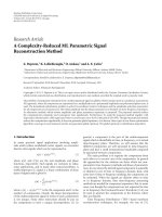
Figure 2: A 2-complex obtained by attaching three tori.
That is, K is obtained by attaching the tori T
1
and T
2
through the longitudinal closed
1-cell and, next, by attaching the longitudinal closed 1-cell of the torus T
3
into the meridional
closed 1-cell of the torus T
2
.
Each torus T
i
is imbedded into K so that
T
1
∩ T
2
α
1
α
2
, T
2
∩ T
3
α
3
β
2
, T
1
∩ T
3
T
1
∩ T
2
∩ T
3
e
0
, 2.4
where e
0
is the unique 0-cell of K, corresponding to 0-cells of T
1
, T
2
,andT
3
through
the identifications. The 2-dimensional CW complex K is illustrate, in Figure 2.
Henceforth, we write T
i
to denote the image of the original torus T
i
into the 2-
complexo K through the identifications above.
Certainly, there are homeomorphisms h
21
: T
2
→ T
1
and h
32
: T
3
→ T
2
with
h
21
|
T
1
∩T
2
identity map and h
32
|
T
2
∩T
3
identity map such that h
21
carries β
2
onto β
1
,and
h
32
carries β
3
onto α
2
. Thus, given a point x
3
∈ β
3
we have h
32
x
3
∈ α
1
T
1
∩ T
2
. We should
use this fact later.
Let
f
1
: T
1
→ T
2
be an arbitrary homeomorphism carrying longitude into longitude
and meridian into meridian. Define
f
2
f
1
◦ h
21
: T
2
→ T
2
and note that
f
2
x
f
1
x for
x ∈ T
1
∩ T
2
. Now, define
f
3
f
2
◦ h
32
: T
3
→ T
2
and note that
f
3
x
f
2
x for x ∈ T
2
∩ T
3
.
In particular,
f
1
e
0
f
2
e
0
f
3
e
0
.Thus,
f
1
,
f
2
,and
f
3
can be used to define a map
f : K → T
2
such that
f|
T
i
f
i
for i 1, 2, 3.
Let p
2
: T
2
→ T
2
be an arbitrary double covering. We can consider, e.g., the
longitudinal double covering p
2
zz
2
1
,z
2
for each z z
1
,z
2
∈ S
1
× S
1
∼
T
2
.
We define the map f : K → T
2
to be the composition f p
2
◦
f.
In order to use Proposition 2.3 to study the Nielsen root classes of f using the
information about
f, we need to prove that f
#
π
1
Kp
2
#
π
1
T
2
.Now,sincef
#
p
2
#
◦
f
#
,
it is sufficient to prove that
f
#
is an epimorphism. This is what we will do. Consider the
composition
f ◦ l : T
1
→ T
2
, where l : T
1
→ K is the obvious inclusion. This composition is
exactly the homeomorphism
f
1
, and therefore the induced homomorphism
f
#
◦ l
#
f
1
#
is
an isomorphism. It follows that
f
#
is an epimorphism. Therefore, we can use Proposition 2.3.
Let a fe
0
∈ T
2
,andletp
−1
2
a{a, a
} be the fiber of p
2
over a. If p
2
is the
longitudinal double covering, as above, then if a a
1
, a
2
, we have a
−a
1
, a
2
.
Clearly, the homomorphism
f
∗
: H
2
K → H
2
T
2
is surjective, with H
2
K ≈ Z
3
and
H
2
T
2
≈ Z. Hence, every map from K into T
2
homotopic to f is surjective. It follows that, for
every map g : K → T
2
homotopic to
f, we have g
−1
a
/
∅ and g
−1
a
/
∅.ByProposition 2.3,
Fixed Point Theory and Applications 7
f
−1
a and
f
−1
a
are Nielsen root classes of f, and both are essential classes. Therefore,
Nf2.
Now, since a fe
0
, either e
0
∈
f
−1
a or e
0
∈
f
−1
a
. Without loss of generality,
suppose that e
0
∈
f
−1
a. Then, by the definition of
f, we have
f
−1
a{e
0
}.Thus,oneof
the Nielsen root classes is unitary. Furthermore, since such class is essential, it follows that its
minimal cardinality is equal to one. Therefore, μ
C
f1.
In order to prove that μf3, note that since each restriction
f|
T
i
is a
homeomorphism and p
2
: T
2
→ T
2
is a double covering, for each map g homotopic
to f, the equation gxa must have at least two roots in each T
i
, i 1, 2, 3. By the
decomposition of K,thisimpliesthatμf ≥ 3. Now, let x
3
be a point in β
3
, x
3
/
e
0
.As
we have seen, h
32
x
3
∈ α
1
⊂ T
1
∩ T
2
.Writex
12
h
32
x
3
. By the definition of
f, we have
fx
12
fx
3
/
fe
0
. Denote y
0
fe
0
and y
1
fx
12
.
Let a ∈ T
2
be a point, and let p
−1
2
a{a, a} be the fiber of p
2
over a. Since T
2
is a
surface, there is a homeomorphism h : T
2
→ T
2
homotopic to the identity map such that
hy
0
a and hy
1
a
.Letq
2
: T
2
→ T
2
be the composition q
2
p
2
◦ h,andletϕ : K → T
2
be the composition ϕ q
2
◦
f. Then, ϕ is homotopic to f and ϕ
−1
a{e
0
,x
12
,x
3
}. Since
μf ≥ 3, this implies that μf3.
Moreover, it is very easy to see that μ
f 1, with the pair
f,
fe
0
providing μ
f .
Note that in this example, for every pair ϕ, a providing μfwhich is equal to 3,we
have necessarily ϕ
−1
a{e
0
,x
1
,x
2
} with either x
1
∈ α
1
and x
2
∈ β
3
or x
1
∈ β
1
and x
2
∈ β
2
.
For the same complex K of Example 2.5, we can construct a similar example with the
range of f being the Klein bottle. The arguments here are similar to the previous example,
and so we omit details.
Example 2.6. Let
p
2
: T
2
→ RP
2
#RP
2
be the orientable double covering. We will construct a
2-dimensional CW complex K and a map f : K → RP
2
#RP
2
having a lifting
f : K → T
2
through p
2
and satisfying the following:
i Nf2,
ii μ
C
f1,
iii μf3,
iv μ
f1.
We repeat the previous example replacing the double covering p
2
: T
2
→ T
2
by the
orientable double covering
p
2
: T
2
→ RP
2
#RP
2
. Also here, we have μ
f1, with the pair
f,
fe
0
providing μ
f.
Small adjustments in the construction of the latter two examples are sufficient to prove
the following theorem.
Theorem 2.7. Let K be the 2-dimensional CW complex of the previous two examples. For each positive
integer n, there are cellular maps f
n
: K → T
2
and g
n
: K → RP
2
RP
2
satisfying the following:
1 Nf
n
n, μ
C
f
n
1 and μf
n
2n − 1.
2 Ng
n
2n, μ
C
g
n
1 and μg
n
4n − 1.
8 Fixed Point Theory and Applications
Proof. In order to prove item 1,let
f : K → T
2
be as in Example 2.5.Letp
n
: T
2
→ T
2
be an n-fold covering which certainly exists; e.g., for each z ∈ T
2
considered as a pair z
z
1
,z
2
∈ S
1
× S
1
, we can define p
n
zz
n
1
,z
2
. Define f
n
p
n
◦
f : K → T
2
. Then, the same
arguments of Example 2.5 can be repeated to prove the desired result.
In order to prove item 2,let
f : K → T
2
be as in Example 2.6.Letp
n
: T
2
→ T
2
be
an n-fold covering e.g., as in the first item,andlet
p
2
: T
2
→ RP
2
#RP
2
be the orientable
double covering. Define q
2n
: T
2
→ RP
2
#RP
2
to be the composition q
2n
p
2
◦ p
n
. Then q
2n
is
a2n-fold covering. Define f
n
q
2n
◦
f : K → RP
2
#RP
2
. Now proceed with the arguments of
Example 2.6.
Observation 2.8. It is obvious that if m and n are different positive integers, then the maps
f
m
,f
n
and g
m
,g
n
satisfying the previous theorem are such that f
m
is not homotopic to f
n
and
g
m
is not homotopic to g
n
.
3. Roots of Liftings through Coverings
In the previous section, we saw several examples of maps from 2-dimensional CW complexes
into closed surfaces having lifting through some covering space and not having all Nielsen
root classes with minimal cardinality. In this section, we study the relationship between the
minimal number of roots of a map and the minimal number of roots of one of its liftings
through a covering space, when such lifting exists.
Throughout this section, M and N are topological n-manifolds either compact or
triangulable, and X denotes a compact, connected, locally path connected, and semilocally
simply connected spaces All these assumptions are true, for example, if X is a finite and
connected CW complex.
Lemma 3.1. Let p
k
: Y → Y be a k-fold covering, and let f : X → Y be a map having a lifting
f : X →
Y through p
k
.Leta ∈ Y be a point, and let p
−1
k
a{a
1
, ,a
k
} be the fiber of p
k
over a.
Then μf, a ≥
k
i1
μ
f,a
i
.
Proof. Let ϕ : X → Y be a map homotopic to f such that #ϕ
−1
aμf, a. Then, since p
k
is a covering, we may lift ϕ through p
k
to a map ϕ : X → Y homotopic to
f. It follows that
ϕ
−1
a∪
k
i1
ϕ
−1
a
i
, with this union being disjoint, and certainly #ϕ
−1
a
i
≥ μ
f,a
i
for all
1 ≤ i ≤ k. Therefore,
μ
f, a
#
k
i1
ϕ
−1
a
i
≥
k
i1
μ
f,a
i
. 3.1
Theorem 3.2. Let p
k
: M → N be a k-fold covering, and let f : X → N be a map having a lifting
f : X → M through p
k
.Thenμf ≥ kμ
f. Moreover, μf0 if and only if μ
f0.
Proof. Let a ∈ N be an arbitrary point, and let p
−1
k
a{a
1
, ,a
k
} be the fiber of p
k
over a.
Since M and N are manifolds, we have μfμf, a and μ
fμ
f,a
i
for all 1 ≤ i ≤ k.
Hence, by the previous lemma, μf ≥ kμ
f. It follows that μ
f0ifμf0. On the
other hand, suppose that μ
f0. Then N
f0andby8, Theorem 2.3, there is a map
Fixed Point Theory and Applications 9
g : X → M homotopic to
f such that dim gX ≤ n − 1, where n is the dimension of M
and N.Letϕ : X → N be the composition ϕ p
k
◦ ϕ. Then ϕ is homotopic to f and
dim ϕX ≤ n − 1. Therefore μf0.
Note that if in the previous theorem we suppose that k 1, then the covering p
k
:
M → N is a homeomorphism and μfμ
f.
In Examples 2.4, 2.5,and2.6 of the previous section, we presented maps f : K → N
from 2-dimensional CW complexes into closed surfaces here N is the projective plane, the
torus, and the Klein bottle, resp. for which we have
μ
f
≥ 3 > 2 2μ
f
. 3.2
This shows that there are maps f : K → N from 2-dimensional CW complexes into
closed surfaces having liftings
f : K → M through a double covering p
2
: M → N and
satisfying the strict inequality
μ
f
> 2μ
f
. 3.3
Moreover, Theorem 2.7 shows that there is a 2-dimensional CW complex K such that,
for each integer n>1, there is a map f
n
: K → T
2
and a map g
n
: K → RP
2
#RP
2
having
liftings
f
n
: K → T
2
through an n-fold covering p
n
: T
2
→ T
2
and g
n
: K → T
2
through a
2n-fold covering q
2n
: T
2
→ RP
2
#RP
2
, respectively, satisfying the relations μf
n
2n − 1 >
n nμ
f
n
and μg
n
4n − 1 < 2n 2nμg
n
.
The proofs of the latter two theorems can be used to create a necessary and sufficient
condition for the identity μfkμ
f to be true. We show this after the following lemma.
Lemma 3.3. Let p
k
: M → N be a k-fold covering, let a
1
, ,a
k
be different points of M, and let
a ∈ N be a point. Then, there is a k-fold covering q
k
: M → N isomorphic and homotopic to p
k
such
that q
−1
k
a{a
1
, ,a
k
}.
Proof. Let p
−1
k
a{b
1
, ,b
k
} be the fiber of p
k
over a. It can occur that some a
i
is equal to
some b
j
. In this case, up to reordering, we can assume that a
i
b
i
for 1 ≤ i ≤ r and a
i
/
b
i
for
i>r, for some 1 ≤ r ≤ k.Ifa
i
/
b
j
for any i, j, then we put r 0. If r k, then there is nothing
to prove. Then, we suppose that r
/
k. For each i r 1, ,k,letU
i
be an open subset of
M homeomorphic to an open n-ball, containing a
i
and b
i
and not containing any other point
a
j
and b
j
.Leth
i
: M → M be a homeomorphism homotopic to the identity map, being the
identity map outside U
i
and such that h
i
a
i
b
i
.Leth : M → M be the homeomorphism
h h
k
◦···◦h
r1
. Then h is homotopic to the identity map and ha
i
b
i
for each 1 ≤ i ≤ k.
Let q
k
: M → N be the composition q
k
p
k
◦ h. Then q
k
is a k-fold covering isomorphic and
homotopic to p
k
. Moreover, q
−1
k
a{a
1
, ,a
k
}.
Theorem 3.4. Let p
k
: M → N be a k-fold covering, and let f : X → N be a map having a lifting
f : X → M through p
k
.Thenμfkμ
f if and only if, for each pair ϕ, a providing μf,each
pair ϕ, a
i
provides μ
f,where ϕ is a lifting of ϕ homotopic to
f and p
−1
k
a{a
1
, ,a
k
}.
10 Fixed Point Theory and Applications
Proof. Let ϕ, a be a pair providing μf,letp
−1
k
a{a
1
, ,a
k
} be the fiber of p
k
over a,and
let ϕ be a lifting of ϕ homotopic to
f. Then ϕ
−1
a∪
k
i1
ϕ
−1
a
i
, with this union being disjoint.
Hence μf
k
i1
#ϕ
−1
a
i
.Now,#ϕ
−1
a
i
≥ μ
f for each 1 ≤ i ≤ k. Therefore, μfkμ
f
if and only if # ϕ
−1
a
i
μ
f for each 1 ≤ i ≤ k, that is, each pair ϕ, a
i
provides μ
f.
Theorem 3.5. Let p
k
: M → N be a k-fold covering, and let f : X → N be a map having a
lifting
f : X → M through p
k
.Thenμfkμ
f if and only if, given k different points of M,say
a
1
, ,a
k
, there is a map ϕ : X → M such that, for each 1 ≤ i ≤ k: the pair ϕ, a
i
provides μ
f.
Proof. Let ϕ, a be a pair providing μf,andletq
k
: M → N be a covering isomorphic and
homotopic to p
k
, such that q
−1
k
a{a
1
, ,a
k
},asinLemma 3.3.
Suppose that μfkμ
f.Let ϕ : X → M be a lifting of ϕ through q
k
homotopic to
f. Then, by the previous theorem, ϕ, a
i
provides μ
f for each 1 ≤ i ≤ k.
On the other hand, suppose that there is a map ϕ : X → M such that, for each 1 ≤ i ≤ k,
the pair ϕ, a
i
provides μ
f.Letϕ : X → N be the composition ϕ q
k
◦ ϕ. Then ϕ is a
lifting of ϕ through q
k
homotopic to
f and μf ≤ #ϕ
−1
a
k
i1
#ϕ
−1
a
i
kμ
f. But, by
Theorem 3.2, we have μf ≥ kμ
f. Therefore μfkμ
f.
Theorem 3.6. Let p
k
: M → N be a k-fold covering, and let f : X → N be a map having a lifting
f : X → M through p
k
.Thenμf >kμ
f if and only if, for every map ϕ : X → M homotopic to
f, there are at most k − 1 points in M whose preimage by ϕ has exactly μ
f points.
Proof. From Theorem 3.2, μ f
/
kμ
f if and only if μf >kμ
f. Thus, a trivial argument
shows that this theorem is equivalent to Theorem 3.5.
Example 3.7. Let f : K → N, p
2
: M → N and
f : K → M be the maps of Examples 2.4,
2.5,or2.6. Then, we have proved that μf ≥ 3 > 2 2μ
f. More precisely, in Examples
2.5 and 2.6 we have μf3. Therefore, by Theorem 3.6,if ϕ : K → M is a map providing
μ
fwhich is equal to 1, then there is a unique point of M whose preimage by ϕ is a single
point.
Now, we present a proposition showing equivalences between the vanishing of the
Nielsen numbers and the minimal number of roots of f and its liftings
f through a covering.
Proposition 3.8. Let p
k
: M → N be a k-fold covering, and let f : X → M be a map having a
lifting
f : X → M through p
k
. Then, the following statements are equivalent:
i Nf0,
ii N
f0,
iii μf0,
iv μ
f0.
Proof. First, we should remember that, by Theorem 3.2, iii⇔iv.Also,sinceNg ≤ μg
for every map g, it follows that iii⇒i and iv⇒ii. On the other hand, by 8, Theorem
2.1, we have that i⇒iii and ii⇒iv. This completes the proof.
Fixed Point Theory and Applications 11
Until now, we have studied only the cases in which a given map f has a lifting through
a finite fold covering. When f has a lifting through an infinite fold covering, the problem is
easily solved using the results of Gonc¸alves and Wong presented in 8.
Theorem 3.9. Let f : X → N be a map having a lifting
f : X → M through an infinite fold
covering p
∞
: M → N. Then the numbers Nf, N
f, μf and μ
f are all zero.
Proof. Certainly, the subgroup f
#
π
1
X has infinite index in the group π
1
N.Thus,by8,
Corollary 2.2, μf0andsoNf0. Now, it is easy to check that also μ
f0andso
N
f0.
4. Minimal Classes versus Roots of Liftings
In this section we present some results relating the problems of Sections 2 and 3.Westart
remembering and proving general results which will be used in here.
Also in this section, X is always a compact, connected, locally path connected and
semilocally simply connected space and M and N are topological n-manifolds either compact
or triangulable.
Let f : X → Y be a map with Y having the same properties of X. We denote the
Riedemeister number of f by Rf, which is defined to be the index of the subgroup f
#
π
1
X in
the group π
1
M. In symbols, Rf|π
1
M : f
#
π
1
X|. When Y is a topological manifold
not necessarily compact, it follows from 2 that Nf > 0 ⇒ NfRf < ∞.Thus,if
Rf∞, then Nf0.
Corollary 4.1. Let f : X → N be a map with Rfk,letp
k
: M → N be a k-fold covering and
let
f : X → M be a lifting of f through p
k
. Then the following statements are equivalent:
i Nf
/
0,
ii Nfk,
iii μf
/
0,
iv μ
f
/
0.
Proof. The equivalences i⇔iii⇔iv are proved in Proposition 3.8. The implication ii⇒i
is trivial. For a proof that i implies ii see 2.
Theorem 4.2. Let p
k
: M → N be a k-fold covering, and let f : X → N be a map having a lifting
f : X → M.IfRfk,thenμ
fμ
C
f.
Proof. If Nf0, then all μf, μ
f,andμ
C
f also are zero. In this case, there is nothing to
prove. Now, suppose that Nf
/
0. Then, by Corollary 4.1, Nfk and μ f and μ
f are
both nonzero. Thus, also μ
C
f
/
0. Let R be a Nielsen root class of f,andletH : f f
1
be a
homotopy starting at f and ending at f
1
. Moreover, let R
1
be the Nielsen root class of f
1
that
is H-related with R.Let
f
1
be a lifting of f
1
through p
k
homotopic to
f.ByProposition 2.3,
R
1
f
−1
1
a for some point a ∈ M over a specific point a of N. Thus, the cardinality #R
1
is
minimal if and only if the cardinality #
f
−1
1
a is minimal; that is, #R
1
μ
C
f if and only if
#
f
1
aμ
f.
12 Fixed Point Theory and Applications
Theorem 4.3. Let p
k
: M → N be a k-fold covering, and let f : X → N be a map having a lifting
f : X → M through p
k
.IfRfk, then the following statements are equivalent:
i μfμ
C
fNf,
ii μfkμ
f,
iii μfμ
fNf.
Proof. By the previous results, we have Nf0 ⇔ μf0 ⇔ μ
f0. Thus, if one
of these numbers are zero, then the three statements are automatically equivalent. Now, if
Nf
/
0, then NfRfk and, by Theorem 4.2, μ
fμ
C
f. This proves the desired
equivalences.
5. Maps into the Projective Plane
In this section, we use the capital letter K to denote finite and connected 2-dimensional CW
complexes, and we use M to denote closed surfaces.
In the next two lemmas, we consider the 2-sphere in the domain of f with cellular
decomposition S
2
e
0
∪ e
2
and the 2-sphere in the range of f with cellular decomposition
S
2
e
0
∗
∪ e
2
∗
.
Lemma 5.1. Let f : S
2
→ S
2
be a map with degree d
/
0, and let a ∈ S
2
be a point, a
/
e
0
∗
. Then,
there is a cellular map ϕ : S
2
→ S
2
such that f ϕ rel{e
0
} and #ϕ
−1
a1 #ϕ
−1
−a.
Proof. Without loss of generality, suppose that a is the north pole and so −a is the south pole.
There is a cellular map g : S
2
→ S
2
such that g f and #g
−1
a1 #g
−1
−a. In fact,
consider the domain sphere S
2
fragmented in |d| southern tracks by meridians m
1
, ,m
|d|
chosen so that e
0
is in m
1
.Letg : S
2
→ S
2
be a map defined so that each meridian m
i
,for
1 ≤ i ≤|d|, is carried homeomorphically onto a same distinguished meridian m of the range 2-
sphere containing e
0
∗
, and each of the |d| tracks covers once the sphere S
2
, always in the same
direction, which is chosen according to the orientation of S
2
,sothatg is a map of degree d.
Since f and g have the same degree, they are homotopic. Moreover, g
−1
a{b} and
g
−1
−a{−b}, where b is the north pole of the domain 2-sphere, and so −b is its south pole.
Therefore, we have #g
−1
a1 #g
−1
−a. What we cannot guarantee immediately is that
the homotopy between f and g is a homotopy relative to {e
0
}.
Now, if H : S
2
× I → S
2
is a homotopy starting at f and ending at g, then as in 9,
Lemma 3.1, we can slightly modify H in a small closed neighborhood V × I of e
0
× I,with
V homeomorphic to a closed 2-disc and not containing a and −a, to obtain a new homotopy
H : S
2
× I → S
2
, which is relative to e
0
.Letϕ : S
2
→ S
2
be the end of this new homotopy,
that is, ϕ
H·, 1. Since H and
H differ only on V × I and a and −a do not belong to V ,we
have ϕ
−1
a{b} and ϕ
−1
−a{−b}.
This concludes the proof of this lemma.
Lemma 5.2. Let f : S
2
→ S
2
be a map with zero degree and let κ
0
: S
2
→ S
2
be the constant map
at e
0
∗
.Thenf κ
0
rel{e
0
}. Moreover, if a ∈ S
2
, a
/
e
0
∗
,thenκ
0
−1
a∅ κ
0
−1
−a.
Proof. This is 9, Lemma 3.2. Also, it is an adaptation of the proof of the previous lemma.
Fixed Point Theory and Applications 13
Now, we insert an important definition about the type of maps which provides the
minimal number of roots of a given map.
Definition 5.3. Let f : K → M be a map. We say that f is of type ∇
2
if there is a pair ϕ, a
providing μf such that ϕ
−1
a ⊂ K \ K
1
. Moreover, we say that f is of type ∇
3
if in addition
we can choose the map ϕ being a cellular map.
Proposition 5.4. Every map f : K → M of type ∇
2
is also of the type ∇
3
.
Proof. Let ϕ : K → M be a map and let a ∈ M be a point such that ϕ, a provides μf
and ϕ
−1
a ⊂ K \ K
1
. We can assume that a is in the interior of the unique 2-cell of M. We
consider M with a minimal cellular decomposition. Let V be an open neighborhood of a in
M homeomorphic to an open 2-disc and such that the closure
V of V in M is contained in
M \ M
1
, where M
1
is the 1-skeleton of M.Letχ : D
2
→ M be the attaching map of the 2-cell
of M,andleth :
V → D
2
be a homeomorphism, where D
2
is the unitary closed 2-disc.
Certainly, there is a retraction r : M \ V → M
1
such that for each x ∈ ∂V we have
rxχ ◦ hx. Then, the maps r and χ ◦ h can be used to define a map g : M → M such
that g|
M\V
r and g|
V
χ ◦ h. Now, it is easy to see that g is cellular and homotopic to the
identity map id : M → M.
Let ψ : K → M be the composition ψ g ◦ ϕ and call a
ga. Then, ψ is a cellular
map homotopic to f and ψ
−1
a
ϕ
−1
a ⊂ K \ K
1
. This concludes the proof.
Proposition 5.5. Every map between closed surfaces is of type ∇
2
and so of type ∇
3
.
Proof. Let f : M → N be a map between closed surfaces. Suppose that n μf,andlet
ϕ, a be a pair providing μf.Letϕ
−1
a{x
1
, ,x
n
}. If each x
j
is in the interior of the
2-cell of M, then there is nothing to prove. Otherwise, let y
1
, ,y
n
be n different points of
M belonging to its 2-cell. There is a homeomorphism h : M → M homotopic to the identity
map id : M → M such that hy
j
x
j
for each 1 ≤ j ≤ n.Letψ : M → N be the composition
ψ ϕ ◦ h. Then ψ is homotopic to f and ψ
−1
a{y
1
, ,y
n
}⊂M \ M
1
.Now,weusethe
previous proposition to complete the proof.
Theorem 5.6. Let f : K → RP
2
be a map having a lifting
f : K → S
2
through the double covering
p
2
: S
2
→ RP
2
.If
f is of type ∇
2
,then2μ
fμfμ
C
fNf.
Proof. Since
f is of type ∇
2
, then
f is also of type ∇
3
,byProposition 5.4.Let ϕ : K → S
2
be a
cellular map, and let a ∈ S
2
e
0
∗
∪ e
2
∗
be a point different from e
0
∗
such that #ϕ
−1
aμ
f and
ϕ
−1
a ⊂ K \ K
1
.Lete
2
1
, ,e
2
m
be the 2-cells of K. For each 1 ≤ i ≤ m, we define the quotient
map
ω
i
: K
K
K \ e
2
i
, 5.1
which collapses the complement of the interior of the 2-cell e
2
i
to a point c
0
i
. The image ω
i
K
K/K \ e
2
i
is naturally homeomorphic to a 2-sphere S
2
i
which inherits from K a cellular
decomposition S
2
i
c
0
i
∪ c
2
i
, where the interior of the 2-cell c
2
i
corresponds homeomorphically
to the image by ω
i
of the interior of the 2-cell e
2
i
of the 2-complex K.
14 Fixed Point Theory and Applications
Since ϕ : K → S
2
is a cellular map, the 1-skeleton K
1
of K is carried by ϕ into the
0-cell e
0
∗
of S
2
. Moreover, K
1
is carried by ω
i
which is also a cellular map into the 0-cell c
0
i
of
the sphere S
2
i
, for all 1 ≤ i ≤ m. Then we can define, for each 1 ≤ i ≤ m, a unique cellular map
ϕ
i
: S
2
i
→ S
2
such that ϕ|
e
2
i
ϕ
i
◦ω
i
|
e
2
i
. In fact, for each x ω
i
x ∈ S
2
i
, we define ϕ
i
x ϕx.
Since ϕ is a cellular map, ϕ
i
is well defined and is also a cellular map. Moreover, for each
x ∈ e
2
i
, we have ϕxϕ
i
◦ ω
i
x.
Since ϕ
−1
a ⊂ K \ K
1
,theset ϕ
−1
a is in one-to-one correspondence with the set
∪
m
i1
ϕ
−1
i
a; in fact, we have ϕ
−1
a∪
m
i1
ϕ
i
◦ ω
i
−1
a. Now, by the proof of Theorem 4.1
of 9, for each 1 ≤ i ≤ m, either # ϕ
−1
i
a1or ϕ is homotopic to a constant map. Then,
by Lemmas 5.1 and 5.2, for each 1 ≤ i ≤ m, there is a cellular map ψ
i
: S
2
i
→ S
2
such that
ϕ
i
ψ
i
rel{c
0
i
} and #ψ
−1
i
a# ϕ
−1
i
a#ψ
−1
i
−a.LetH
i
: ϕ
i
ψ
i
rel{c
0
i
} be such homotopies,
1 ≤ i ≤ m.
For each x ∈ K, choose once and for all an index ix ∈{1, ,m} such that x ∈ e
ix
.
Then, define ψ : K → S
2
by ψx ψ
ix
ω
ix
x. This map is clearly well defined and
cellular. Moreover, the homotopies H
i
,1≤ i ≤ m, can be used to define a homotopy H
starting at ϕ and ending at ψ.
From this construction, we have #ψ
−1
aμ
f#ψ
−1
−a.ByTheorem 3.5, we have
that μf2μ
f. Now, it is obvious that Rf2. So, by Theorem 4.3, μfμ
C
fNf.
Theorem 5.6 is not true, in general, when the map f is not of the type ∇
2
. We present
an example to illustrate this fact.
Example 5.7. Let K S
2
1
∨ S
2
2
be the bouquet of two 2 spheres with minimal cellular
decomposition with one 0-cell e
0
and two 2-cells e
2
1
and e
2
2
.Let
f : K → S
2
be a map which,
restricted to each S
2
i
, i 1, 2, is homotopic to the identity map. Consider the sphere S
2
with
its minimal cellular decomposition S
2
e
0
∗
∪ e
2
∗
. Then, there is a cellular map ϕ : K → S
2
homotopic to
f such that ϕ
−1
e
0
∗
{e
0
}.Thus,thepair ϕ, e
0
∗
provides μ
f1, of course.
Now, it is obvious that ,for every map g homotopic to
f, the restrictions g|
S
2
i
, i 1, 2, are
surjective. Hence, for every such map g, the equation gxa has at least one root in each
S
2
i
, i 1, 2, whatever the point a ∈ S
2
. Therefore, if x
0
is a root of gxa belonging to the
interior of one of the 2 cells of K, then the equation gxa must have a second root, which
must belong to the closure of the other 2 cell of K. But in this case, #g
−1
a ≥ 2, and so the
pair g,a do not provide μ
f. This means that the map
f is not of type ∇
2
. Moreover, this
shows that if ϕ, a is a pair providing μ
f , then necessarily ϕ
−1
a{e
0
}. Thus, for every
map ϕ : K → S
2
homotopic to
f, there is at most one point in S
2
whose preimage by ϕ is
a set with μ
f points. Now, let p
2
: S
2
→ RP
2
be a double covering, and let f : K → RP
2
be the composition f p
2
◦
f. Then
f is a lifting of f through p
2
,and,byTheorem 3.6,we
have μf > 2μ
f. More precisely, μf3. Moreover, μ
C
f1, Nf2andμf
/
μ
C
fNf.
In the next theorem, Af denotes the absolute degree of the given map f see 10 or
11.
Theorem 5.8. Let f : M → RP
2
be a map inducing the trivial homomorphism on fundamental
groups. Then, μf0 if Af0 and μf2 if Af
/
0.
Fixed Point Theory and Applications 15
Proof. Since f
#
π
1
M is trivial, f has a lifting
f : M → S
2
through the universal double
covering p
2
: S
2
→ RP
2
.ByProposition 5.5,
f is of type ∇
2
. Hence, by Theorem 5.6, we have
μf2μ
f. Now, it is well known that μ
f0ifA
f0andμ
f1ifA
f
/
0. see,
e.g., 11 or 9 or 3. But, by the definition of absolute degree see 11, page 371 it is easy
to check that Af2A
f. This concludes the proof.
Theorem 5.8 is not true, in general, if the homomorphism f
#
: π
1
M → π
1
RP
2
is
not the trivial homomorphism. To illustrate this, let id : RP
2
→ RP
2
be the identity map.
It is obvious that this map induces the identity isomorphism on fundamental groups and
μid1.
In the next theorem, X is a compact, connected, locally path connected, and semilocally
simply connected space.
Theorem 5.9. Let f : X → RP
2
be a map. Then μfμ
C
fNf if at least one of the following
alternatives is true: < (i) f
#
π
1
X
/
0; (ii) X is a 2-dimensional CW complex, and f is of type ∇
2
.
Proof. Up to isomorphism, there are only two covering spaces for RP
2
, namely, the identity
covering p
1
: RP
2
→ RP
2
and the double covering p
2
: S
2
→ RP
2
. Suppose that i is true.
Then, f
#
π
1
Xπ
1
RP
2
≈ Z
2
,andp
1
is a covering corresponding to f
#
π
1
X. Thus, either
Nf0orNfRf1. Now, if Nf0, then also μf0byProposition 3.8.If
Nf1, then the result is obvious. Therefore, we have μfμ
C
fNf. If, on the other
hand, ii is true and i is false, then we use Theorem 5.6.
Example 5.7 shows that the assumptions in Theorem 5.9 are not superfluous.
Acknowledgments
The authors would like to express their thanks to Daciberg Lima Gonc¸alves for his
encouragement to the development of the project which led up to this article. This work
is partially sponsored by FAPESP - Grant 2007/05843-5. They would like to thank the referee
for his careful reading, comments, and suggestions which helped to improve the manuscript.
References
1 D. L. Gonc¸alves, “Coincidence theory,” in Handbook of Topological Fixed Point Theory,R.F.Brown,M.
Furi, L. G
´
orniewicz, and B. Jiang, Eds., pp. 3–42, Springer, Dordrecht, The Netherlands, 2005.
2 R. Brooks, “Nielsen root theory,” in Handbook of Topological Fixed Point Theory,R.F.Brown,M.Furi,L.
G
´
orniewicz, and B. Jiang, Eds., pp. 375–431, Springer, Dordrecht, The Netherlands, 2005.
3 D. L. Gonc¸alves and C. Aniz, “The minimizing of the Nielsen root classes,” Central European Journal of
Mathematics, vol. 2, no. 1, pp. 112–122, 2004.
4 J. Jezierski, “Nielsen number of a covering map,” Fixed Point Theory and Applications, vol. 2006, Article
ID 37807, 11 pages, 2006.
5 C. Aniz, Ra
´
ızesdefunc¸
˜
oes de um Complexo em uma Variedade, M.S. thesis, ICMC, Universidade de S
˜
ao
Paulo, S
˜
ao Carlos, Brazil, 2002.
6 L. Xiaosong, “On the root classes of a mapping,” Acta Mathematica Sinica, vol. 2, no. 3, pp. 199–206,
1986.
7 M. A. Armstrong, Basic Topology, Undergraduate Texts in Mathematics, Springer, New York, NY, USA,
1983.
8 D. L. Gonc¸alves and P. Wong, “Wecken property for roots,” Proceedings of the American Mathematical
Society, vol. 133, no. 9, pp. 2779–2782, 2005.
16 Fixed Point Theory and Applications
9 M. C. Fenille and O. M. Neto, “Roots of maps from 2-complexes into the 2-sphere,” preprint, 2009.
10 R. F. Brown and H. Schirmer, “Nielsen root theory and Hopf degree theory,” Pacific Journal of
Mathematics, vol. 198, no. 1, pp. 49–80, 2001.
11 D. B. A. Epstein, “The degree of a map,” Proceedings of the London Mathematical Society, vol. 16, no. 1,
pp. 369–383, 1966.