báo cáo hóa học:" Research Article Performance Evaluation of UML2-Modeled Embedded Streaming Applications with System-Level Simulation" pdf

Hindawi Publishing Corporation
EURASIP Journal on Embedded Systems
Volume 2009, Article ID 826296, 16 pages
doi:10.1155/2009/826296

Research Article
Performance Evaluation of UML2-Modeled Embedded Streaming
Applications with System-Level Simulation
Tero Arpinen, Erno Salminen, Timo D. Hă mă lă inen, and Marko Hă nnikă inen
a aa
a
a
Department of Computer Systems, Tampere University of Technology, P.O. Box 553, 33101 Tampere, Finland
Correspondence should be addressed to Tero Arpinen, tero.arpinen@tut.fi
Received 27 February 2009; Accepted 21 July 2009
Recommended by Bertrand Granado
This article presents an efficient method to capture abstract performance model of streaming data real-time embedded systems
(RTESs). Unified Modeling Language version 2 (UML2) is used for the performance modeling and as a front-end for a tool
framework that enables simulation-based performance evaluation and design-space exploration. The adopted application metamodel in UML resembles the Kahn Process Network (KPN) model and it is targeted at simulation-based performance evaluation.
The application workload modeling is done using UML2 activity diagrams, and platform is described with structural UML2
diagrams and model elements. These concepts are defined using a subset of the profile for Modeling and Analysis of Realtime and
Embedded (MARTE) systems from OMG and custom stereotype extensions. The goal of the performance modeling and simulation
is to achieve early estimates on task response times, processing element, memory, and on-chip network utilizations, among other
information that is used for design-space exploration. As a case study, a video codec application on multiple processors is modeled,
evaluated, and explored. In comparison to related work, this is the first proposal that defines transformation between UML activity
diagrams and streaming data application workload meta models and successfully adopts it for RTES performance evaluation.
Copyright © 2009 Tero Arpinen et al. This is an open access article distributed under the Creative Commons Attribution License,
which permits unrestricted use, distribution, and reproduction in any medium, provided the original work is properly cited.

1. Introduction
Multiprocessor System-on-Chip (SoC) offers high performance, yet energy-efficient, and programmable platform

for modern embedded devices. However, parallelism and
increasing complexity of applications necessitate efficient
and automated design methods. Model-driven development
(MDD) aims to shorten the design time using abstraction,
gradual refinement, and automated analysis with transformation of models. The key idea is to utilize models to
highlight certain aspects of the system (behavior, structure,
timing, power consumption models, etc.) without an implementation.
Unified Modeling Language version 2 (UML2) [1] is a
standard language for MDD. In embedded system domain,
its adoption is seen promising for several purposes: requirements specification, behavioral and architectural modeling,
test bench generation, and IP integration [2]. However, it
should be noted that UML2 has had also criticism on its
suitability in MDD [3, 4]. UML2 offers a rich set of diagrams
for modeling and also expansion and tailoring methods

to derive domain-specific languages. For example, several
UML profiles targeted at embedded system design have been
developed [5–7].
SoC complexity requires efficient performance evaluation and design-space exploration methods. These methods
are often utilized at the system level to make early design
decisions. Such decisions include, for instance, choosing
the number and type of processors, and determining the
mapping and scheduling of application tasks. Design-space
exploration seeks to find optimum solution for a given
application (domain) and boundary constraints. Design
space, that is, the number of possible system configurations,
is practically always so large that it becomes intractable not
only for manual design but also for brute force optimization.
Hence, efficient methods are needed, for example, optimization heuristics, tool frameworks, and models [8].
This article presents an efficient method to capture

abstract performance model of a streaming data real-time
embedded system (RTES). Figure 1 presents the overall
methodology used in this work. The goal of the performance
modeling and simulation is to achieve early estimates on


2

EURASIP Journal on Embedded Systems
Application
workload modeling
(UML2 activities)

Platform
performance modeling
(UML2 structural)

• Workload Application
functions

Platform
resources

Mapping
System-level simulation
(SystemC)

Design-space exploration
(models and simulation
results)

Execution
monitoring
(simulation results)

Figure 1: The methodology used in this work.

PE, memory, and on-chip network utilization, task response
times, among other information that is used for design-space
exploration. UML2 is used for performance model specification. The application workload modeling is carried out
using UML2 activity diagrams. Platform is described with
structural UML2 diagrams and model elements annotated
with performance values.
Our focus is on modeling streaming data applications.
It is characteristic to streaming applications that a long
sequence of data items flows through a stable set of computation steps (tasks) with only occasional control messaging
and branching. Each task waits for the data items, processes
them, and outputs the results to the next task. The adopted
application metamodel has been formulated based on this
assumption and it resembles Kahn Process Network (KPN)
[9] model.
A proprietary UML2 profile for capturing performance
characteristics of an application and platform is defined.
The profile definition is based on a well-defined metamodel
and reusing suitable modeling concepts from the profile for
Modeling and Analysis of Realtime and Embedded systems
(MARTE) [5]. MARTE is a standard profile promoted
by the Object Management Group (OMG) and it is a
promising extension for general-purpose embedded system
modeling. It has been intended to replace the UML Profile for

Schedulability, Performance and Time (SPT) [10]. MARTE
is methodology-independent and it offers a common set of
standard notations and semantics for a designer to choose
from while still allowing to add custom extensions. This
means that the profile defined in this article is a specialized
instance of the MARTE profile that is dedicated for our
performance evaluation methodology.
It should be noted that the performance models defined
in this work can be and have been used together with a
custom UML profile for embedded systems, called TUTProfile [7, 11]. However, this article illustrates the models using the concepts of MARTE because the adoption
of standards promotes commonly known notations and
semantics between designers and interoperability between
tools.
Further, the article presents how performance values
can be specified on UML models with expressions using
MARTE Value Specification Language (VSL). This allows
effective parameterization of system performance model

Functions on
platform resources

• Processin elements
• Communication elements
• Memory elements
• Binding application workloads
on platform elements
• Performance analysis
• Simulations

Figure 2: Design Y-chart.

representation according to application-specific variables
and reduces the amount of time consuming and error-prone
manual work.
The presented modeling methods are utilized in a
tool framework targeted at simulation-based design-space
exploration and performance evaluation. The exploration is
based on collecting performance statistics from simulation
to optimize the platform and mapping according to a
predefined cost-function.
An execution-monitoring tool provides visualization and
monitoring the system performance during the simulation.
As a case study, a video codec system is modeled with the
presented modeling methods and performance evaluation
and exploration is carried out using the tool framework.
The rest of the article is organized as follows. Section 2
analyses the methods and concepts used in RTES performance evaluation. Section 3 presents the metamodel utilized
in this work for system performance characterization. UML2
and MARTE for RTES modeling are discussed in Section 4.
Section 5 presents the UML2 specification of the utilized performance metamodel. Section 6 presents our performance
evaluation tool framework. The video codec case study is
covered in Section 7. After final discussion on our proposal
in Section 8, Section 9 concludes the article.

2. Analysis of Methods and Concepts Used in
RTES Performance Evaluation
In this section the methods and concepts used in RTES
performance evaluation are covered. This comprises an
introduction to design Y-chart in RTES performance evaluation, phases of a model-based RTES performance evaluation process, discussion on modeling language and tool
development, and a short introduction to RTES timing

analysis concepts. Finally, the related work on UML in RTES
performance evaluation is examined.
2.1. Design Y-Chart and RTES Modeling. Typical approach
for RTES performance evaluation follows the design Y-chart
[12] presented in Figure 2 by separating the application
description from underlying platform description. These two
are bound in the mapping phase. This means that communication and computation of application functionalities are
committed onto certain platform resources.
There are several possible abstraction levels for describing the application and platform for performance evaluation.


EURASIP Journal on Embedded Systems
One possibility is to utilize abstract specifications. This
means that application workload and performance of the
platform resources are represented symbolically without
needing detailed executable descriptions.
Application workload is a quantity which informs how
much capacity is required from the underlying platform
components to execute certain functionality. In model-based
performance evaluation the workloads can be estimated
based on, for example, standard specifications, prior experience from the application domain, or available processing
capacity. Legacy application components, on the other
hand, can be profiled and performance models of these
components can be evaluated together with the models of
components yet to be developed.
In addition to computational demands, communication
demands between application parts must be considered. In
practice, the communication is realized as data messages
transmitted between real-time operating system (RTOS)
threads or between processing elements over an on-chip

communication network. Shared buses and Network-onChip (NoC) links and routers perform scheduling for
transmitted data packets in an analogous way as PEs execute
and schedule computational tasks. Moreover, inter-PE communication can be alternatively performed using a shared
memory. The performance characteristics of memories as
well as their utilization play a major role in the overall system
performance. The impact of computation, communication,
and storage activities should all be considered in systemlevel analysis to enable successful performance evaluation of
a modern SoC.
2.2. Model-Based RTES Performance Evaluation Process.
RTES performance evaluation process must follow disciplined steps to be effective. From SoC designer’s perspective,
a generic performance evaluation process consists of the
following steps. Some of the concepts of this and the next
subsection have been reused and modified from the work in
[13]:
(1) selection of the evaluation techniques and tools,
(2) measuring, profiling, and estimating workload characteristics of application and determining platform
performance characteristics by benchmarking, estimation, and so forth,
(3) constructing system performance model,
(4) measuring, executing, or simulating system performance models,
(5) interpreting, validating, monitoring, and backannotating data received from previous step.
The selection of the evaluation techniques and tools is
the first and foremost step in the performance evaluation
process. This phase includes considering the requirements
of the performance analysis and availability of tools. It
determines the modeling methods used and the effort
required to perform the evaluation. It also determines the
abstraction level and accuracy used. All further steps in the
process are dependent on this step.

3

The second step is performed if the system performance
model requires initial data about application task workloads
or platform performance. This is based on profiling, specifications, or estimation. The application as well as platform
may be alternatively described using executable behavioral
models. In that case, such additional information may not
be needed as all performance data can be determined during
system model execution.
The actual system model is constructed in the third step
by a system architect according to defined metamodel and
model representation methods. Gathered initial performance
data is annotated to the system model. The annotation of
the profiling results can also be accelerated by combining the
profiling and back-annotation with automation tools such as
[14].
After system modeling, the actual analysis of the model
is carried out. This may involve several model transformations, for example, from UML to SystemC. The analysis
methods can be classified into dynamic and static methods
[8]. Dynamic methods are based on executing the system
model with simulations. Simulations can be categorized into
cycle-accurate and system-level simulations. Cycle-accurate
simulation means that the timing of system behavior is
defined by the precision of a single clock cycle. Cycleaccuracy guarantees that at any given clock cycle, the state
of the simulated system model is identical with the state
of the real system. System-level simulation uses higher
abstraction level. The system is represented at IP-block level
consisting coarse grained models of processing, memory,
and communication elements. Moreover, the application
functionality is presented by coarse-grained models such as
interacting tasks.
Static (or analytic) methods are typically used in early

design-space exploration to find different corner cases.
Analytical models cannot take into consideration sporadic
effects in the system behavior, such as aperiodic interrupts
or other aperiodic external events. Static models are suited
for performance evaluation when deterministic behavior of
the system is accurate enough for the analysis.
Static methods are faster and provide significantly larger
coverage of the design-space than dynamic methods. However, static methods are less accurate as they cannot take into
account dynamic performance aspects of a multiprocessor
system. Furthermore, dynamic methods are better suited
for spotting delayed task response times due to blocking of
shared resources.
Analysing, measuring, and executing the system performance models produces usually a massive amount of
data from the modeled system. The final step in the flow
is to select, interpret, and exploit the relevant data. The
selection and interpretation of the relevant data depends
on the purpose of the analysis. The purpose can be early
design-space exploration, for example. In that case, the flow
is usually iterative so that the results are used to optimize the
system models after which the analysis is performed again for
the modified models. In dynamic methods, an effective way
of analysing the system behavior is to visualize the results
of simulation in form of graphs. This helps the designer to
efficiently spot changes in system behavior over time.


4

EURASIP Journal on Embedded Systems

2.3. Modeling Language and Tool Development. SoC designers typically utilize predefined modeling languages and tools
to carry out the performance evaluation process. On the
other hand, language and tool developers have their own
steps to provide suitable evaluation techniques and tools for
SoC designers. In general they are as follows:
(1) formulation of metamodel,
(2) developing methods for model representation and
capturing,
(3) developing analysis tools according to selected modeling methods.
The formulation of the metamodel requires very similar
kind of consideration on the objectives of the performance
analysis as the selection of the techniques and tools by
SoC designers. The created metamodel determines the effort
required to perform the evaluation as well as the abstraction
level and accuracy used. In particular, it defines whether the
system performance model can be executed, simulated, or
statically analysed.
The second step is to define how the model is captured by
a designer. This phase includes the selection or definition of
the modeling language (such as UML, SystemC or a custom
domain-specific language). The selection of notations also
requires transformation rules defined between the elements
of the metamodel and the elements of the selected description language. In case of UML2, the metamodel concepts are
mapped to UML2 metaclasses, stereotyped model elements,
and diagrams.
We want to emphasize the importance of performing
these first two steps exactly in this order. The definition of
the metamodel should be performed independently from
the utilized modeling language and with full concentration
on the primary objectives of the analysis. The selection of

the modeling language should not alter the metamodel nor
bias the definition of it. Instead, the modeling language and
notations should be tailored for the selected metamodel, for
instance, by utilizing extension mechanisms of the UML2
or defining completely new domain-specific language. The
reason for this is that model notations contribute only to
presentational features. Model semantics truly determine
whether the model is usable for the analysis. Nevertheless,
presentational features determine the feasibility of the model
for a human designer.
The final step is the development of the tools. To provide
efficient evaluation techniques, the implementation of the
tools should follow the created metamodel and its original
objectives. This means that the original metamodel becomes
the foundation of the internal metamodel of the tools. The
system modeling language and tools are linked together with
model transformations. These transformations are used to
convert the notations of the system modeling language to the
format understood by the tools, while the semantics of the
model is maintained.
2.4. RTES Timing Analysis Concepts. A typical SoC contains heterogeneous processing elements executing complex
application tasks in parallel. The timing analysis of such a

system requires abstraction and parameterization of the key
concerns related to resulting performance.
Hansson et al. define concepts for RTES timing analysis
[15]. In the following, a short introduction to these concepts
is given.
Task execution time te is the time in which (in clock cycles
or absolute time) a set of sequential operations are executed

undisturbed on a processing element. It should be noted
that the term task is here considered more generally as a
sequence of operations or actions related to single-threaded
execution, communication, or data storing. The term thread
is used to denote typical schedulable object in an RTOS.
profiling the execution time does not consider background
activities in the system, such as RTOS thread pre-emptions,
interrupts, or delays for waiting a blocked shared resource.
The purpose of execution time is to determine how much
computing resources is required to execute the task. Task
response time tr , on the other hand, is the actual time it
takes from beginning to the end of the task in the system.
It accounts all interference from other system parts and
background activities.
Execution time and response time can be further classified into worst case (wc), best case (bc), and average case (ac)
times. Worst case execution time twce is the worst possible
time the task can take when not interfered by other system
activities. On the other hand, worst case response time twcr is
the worst possible time the task may take when considering
the worst case scenario in which other system parts and
activities interfere its execution. In multimedia applications
that require streaming data processing, the worst case and
average case response times are usually the ones needed to
be analysed. However, in some hard real-time systems, such
as a car air bag controller, also the best case response time
(tbcr ) may be as important as the twcr . Average case response
time is usually not so significant. Jitter is a measure for time
variability. For a single task, jitter in execution time can be
calculated as Δte = twce − tbce . Respectively, jitter in response
time can be calculated as Δtr = twce − tbcr .

It is assumed that the execution time is constant for a
given task-PE pair. It should be noted that in practice the
execution time of a function may vary depending on the
processed data, for example. For these kinds of functions
the constant task execution time assumption is not valid.
Instead, different execution times of such functions should
be modeled by selecting a suitable value to characterize it
(e.g., worst or average case) or by defining separate tasks
for different execution scenarios. As opposed to execution
time, response time varies dynamically depending on the
task’s surrounding system it is executed on. The response
time analysis must be repeated if
(1) mapping of application tasks is changed,
(2) new functionalities (tasks) are added to the application,
(3) underlying execution platform is modified,
(4) environment (stimuli from outside) changes.
In contrast, a single task execution time does not have
to be profiled again if the implementation of the task is not


EURASIP Journal on Embedded Systems
changed (e.g., due to optimization) assuming that the PE
on which the profiling was carried out is not changed. If
the PE executing is changed and the profiling uses absolute
time units, then a reprofiling is needed. However, this
can be avoided by utilizing PE-neutral parameters, such as
number of operation, to characterize the execution load
of the task. Other possibility is to represent processing
element performances using a relative speed factor as in
[16].

In multiprocessor SoC performance evaluation, simulating the profiled or estimated execution times (or number of
operations) of tasks on abstract HW resource models is an
effective way of observing combined effects of task execution
times, mapping, scheduling, and HW platform parameters
on resulting task response times, response time jitters, and
processing element utilizations.
Timing requirements of SoC functions are compared
against estimated, simulated, or measured response times.
It is typical that timing requirements are given as combined
response times of several individual tasks. This is naturally
completely dependent on the granularity used in identifying
individual tasks. For instance, a single WLAN data transmission task could be decomposed into data processing,
scheduling, and medium access tasks. Then examining if
the timing requirement of a single data transmission is met
requires examining the response times of the composite tasks
in an additive manner.
2.5. On UML in Simulation-Based RTES Performance Evaluation. Related work has several static and dynamic methods
for performance evaluation of parallel computer systems.
A comprehensive survey on methods and tools used for
design-space exploration is presented in [8]. Our focus is on
dynamic methods and some of the closest related research to
our work are examined in the following.
Erbas et al. [17] present a system-level modeling and simulation environment called Sesame, which aims at efficient
design space exploration of embedded multimedia system
architectures. For application, it uses KPN for modeling
the application performance with a high-level programming
language. The code of each Kahn process is instrumented
with annotations describing the application’s computational
actions, which allows to capture the computational behavior
of an application. The communication behavior of a process

is represented by reading from and writing to FIFO channels.
The architecture model simulates the performance consequences of the computation and communication events
generated by an application model. The timing of application
events are simulated by parameterizing each architecture
model component with a table of operation latencies. The
simulation provides performance estimates of the system
under study together with statistical information such as
utilization of architecture model components. Their performance metamodel and approach has several similarities
with ours. The biggest differences are in the abstraction level
of HW communication modeling and visualization of the
system models and performance results.
Balsamo and Marzolla [18] present how UML use case,
activity and deployment diagrams can be used to derive

5
performance models based on multichain and multiclass
Queuing Networks. The UML models are annotated according to the UML Profile for Schedulability, Performance and
Time Specification [10]. This approach has been developed
for SW architectures rather than for embedded systems. No
specific tool framework is presented.
Kreku et al. [19] propose a method for simulationbased RTES performance evaluation. The method is based
on capturing application workloads using UML2 statemachine descriptions. The platform model is constructed
from SystemC component models that are instantiated
from a library. Simulation is enabled with automatic C++
code generation from UML2 description, which makes the
application and platform models executable in a SystemC
simulator. Platform description provides dedicated abstract
services for application to project its computational and
communicational loads on HW resources. These functions
are invoked from actions of the state-machines. The utilization of UML2 state-machine enables efficiently capturing the

control structures of the application. This is a clear benefit in
comparison to plain data flow graphs. The platform services
can be used to represent data processing and memory
accesses. Their method is well suited for control-intensive
applications as UML state-machines are used as the basis
of modeling. Our method targets at modeling embedded
streaming data applications with less effort required in
modeling using UML activity diagrams.
Madl et al. [20] present how distributed real-time
embedded systems can be represented as discrete event
systems and propose an automated method for verification
of dense time properties of such systems. The model of
computation (MoC) is based on tasks connected with
channels. Tasks are mapped onto machines that represent
computational resources of embedded HW.
Our performance evaluation method is based on executable streaming data application workload model specified
as UML activity diagrams and abstract platform performance model specified in composite structure diagrams. In
comparison to related work, this is the first proposal that
defines transformation between UML activity diagrams and
streaming data application workload models and successfully
adopts it for embedded RTES performance evaluation.

3. Performance Metamodel for
Streaming Data Embedded Systems
The foundations of the performance metamodel defined in
this work is based on the earlier work on Model of Computation (MoC) for architecture exploration described in [21].
We introduce storage tasks, storage elements, and timing
constraints as new features. The metamodel definition is
given using mathematical equations and set theory. Another
alternative would be to utilize Meta Object Facility (MOF)

[22]. MOF is often used to define the metamodels from
which UML profiles are derived as the model elements and
notations of MOF are a subset of UML model elements.
Next, detailed formulation of the performance metamodel is
carried out.


6

EURASIP Journal on Embedded Systems

3.1. Application Performance Metamodel. Application A is
defined as a tuple
A = (T, Δ, E, TC),

(1)

where T is a set of tasks, Δ is a set of channels, E is a set
of external events (or timers), and TC is a set of timing
constraints. Tasks are further categorized to sets of execution
tasks Te and storage tasks Ts , so that
T = {Te ∪ Ts }.

(2)

Channels combine tasks and carry tokens between them. A
single channel δ ∈ Δ is defined as
δ = (τsrc , τend , Ebuf ),

(3)

where τsrc ∈ T is task that emits tokens to the channel, τend ∈
T task that consumes tokens, and Ebuf is the set of buffered
tokens in the channel. Tokens in channels represent the flow
of control as well as flow of data in the application. A token
carries certain amount of data from task to another. This has
two impacts. First, the load on the communication medium
for the time of the transfer. Second, the execution load
when the next task is triggered after reception. Latter enables
data amount-dependent dynamic variations in execution
of application tasks. Similar to traditional KPN model,
channels between tasks (or processes) are uni-directional,
unbounded FIFO buffers and tasks use a blocking read as a
synchronization mechanism.
A task τ ∈ T is defined as
τ = (S, ec, F, Δ! , Δ? ),

(4)

where S ∈ {Run, Ready, Wait, Free} is the state of the task,
ec ∈ {N+ ∪ {0}} is the execution counter that is incremented
by one each time the task is fired, and F is a set firing rules of
which definition depends on the type of the task. However Δ!
is the set of incoming channels to the task and Δ? is the set of
outgoing channels. Incoming channels of task τ are defined as
Δτ
!

= {δ ∈ Δ | τend = τ },

(5)

whereas outgoing channels have definition
Δτ = {δ ∈ Δ | τsrc = τ }.
?

(6)

Firing rule fc ∈ Fc for a computational task is a tuple
fc = (tc, Oint , Ofloat , Omem , Δout ),

tc = Δin , depend, Tec , φec ,

(8)

(9)

where Δin ⊂ Δτ is the set of required incoming transitions to
!
trigger the task τ and depend ∈ {Or, And} determines the
dependency type from incoming transitions. Tec is execution
count modulo period and φec is execution count modulo
phase. They can be used to restrict the firing of the task to
certain execution count values, so that the task is fired if
ec mod φec = 0 when ec < Tec ,
ec mod Tec + φec = 0

when ec ≥ Tec .

(10)

3.2. External Events and Constraints. External events model
the environment of the application feeding input data to the
task graph, such as packet reception from WLAN radio or
image reception from an embedded camera. External event
e ∈ E is a tuple
e = type, tper , δout ,

(11)

where type ∈ {Oneshot, Periodic} determines whether the
event is fired once or periodically. tper is the absolute time or
period when the event is triggered, and δout is the channel
where events are fed.
A path p is a finite sequence of consecutive tasks. Thus, if
n ∈ {N+ ∪ {0}} is the total number of tasks in the path, then
p is defined as n-tuple
p = (x1 , x2 , x3 , . . . , xn ),

∀x : x ∈ {T ∪ Δ}.

(12)

A timing constrain tc ∈ TC is defined
req

req

tc = p, twcr , tbcr ,

(13)

in which p is a consecutive path of tasks and channels and
req
req
twcr and tbcr are the required worst-case response time and
best case response time for the p to be completed after the
first element of p has been triggered.
3.3. Platform Performance Metamodel. The HW platform is
a tuple
PHW = (C, L),

(7)

where tc is a task trigger condition. Oint , Ofloat , and Omem
represent the computational complexity of the task in
terms of amounts of integer, floating point, and memory
operations required to be computed. Subset Δout ⊂ Δ?
determine the set of outgoing channels where tokens are
transmitted when the task is fired. Firing rule fs ∈ Fs for a
storage task is a tuple
fs = (tc, Ord , Owr , Δout ),

where Ord and Owr are the amounts of read and write operations associated to a single storage task. Correspondingly to
execution task, tc is task trigger condition and Δout ⊂ Δ?
is the set of outgoing channels. A task trigger condition is
defined as

(14)

in which C is a set of platform components and L is a set of
communication links connecting components. Components
are further divided into sets of processing elements PE,
storage elements SE, and to a single communication element
ce in such a manner that
C = (PE ∪ SE ∪ ce).

(15)

Links L connect processing and storage elements to the
communication element ce. The ce carries out the required
data exchange between PEs and SEs.


EURASIP Journal on Embedded Systems

e0

δ2

τe

τe4

δ3
δ1

τe1

m0

τe3

m1

τs0

δ4

m2

m3 m4

pe2

se0

Communication

ce

HW platform

pe1

Figure 3: Example performance model.

A processing element pe ∈ PE is defined as
pe = fop , Pint , Pfloat , Pmem ,

(16)

in which fop is the operating frequency, Pint , Pfloat , Pmem
describe the performance indices of the PE in terms of
executing integer, floating, and memory operations, respectively. If a task has operational complexity O (of some of the
three types) and the PE it is mapped on has corresponding
performance index P and frequency fop then task execution
time can be calculated with
te =

O
.
P · fop

(17)

Storage element se ∈ SE is defined as
se = fop , Prd , Pwr ,

(18)

in which Prd and Pwr are performance indices for reading
and writing from and to storage element. The time which it
takes to read or write to the storage is calculated in the same
manner as in (17).
The communication element ce has definition
ce = fop , Ptx ,

(19)

where Ptx is the performance index for transmitting data. If a
token carries n bits of data using the communication element
then the time of the transfer can be calculated as
n
.
ttx =
(20)
Ptx · fop
3.4. Metamodel for Functionality Mapping. The mapping M
binds application load characteristics (tasks and channels) to
platform resources. It is defined as
M = {M e ∪ M s },

where Me = (me1 , me2 , me3 , . . . , men ) is a set of mappings of execution tasks to processing elements, Ms =
(ms1 , ms2 , ms3 , . . . , msn ) mappings of storage tasks to storage
elements. In general, a mapping m ∈ M is defined as 2tuple (task, platform element). For instance, execution task
mapping is defined as
m = τe , pe ,

m5
Computation

pe0

δ5

Application

e1

δ0

τe0

7

(21)

τe ∈ Te ∧ pe ∈ PE.

(22)

Each task is mapped only onto one platform element
and several tasks can be mapped onto a single platform
element. Events are not mapped to any platform element.
The mapping of channels onto communication element is
not explicitly modeled. Instead, they are implicitly mapped
onto the single communication element that interconnects
processing and storage elements.
3.5. Example Model. Figure 3 visualizes the primary concepts
of our metamodel with a simple example. There are five
execution tasks τe0 –τe4 and a single storage task τs0 combined
together with six channels δ0 –δ5 . Two external events e0 and
e1 are feeding the task graph with tokens. Computation tasks
are mapped (m0 –m3 ) onto three PEs and the single storage
task is mapped (m4 ) onto the single storage element. All
channels are implicitly mapped onto the single communication element and all inter-PE transfers are conducted by it.

4. UML2 and the MARTE Profile
UML has been traditionally used for specifying softwareintensive systems but currently it is seen as a promising

language for developing embedded systems as well. Natively
UML2 lacks some of the key concepts that are crucial
for embedded systems such as quantifiable notion of time,
nonfunctional properties, embedded execution platform,
and mapping of functionality. However, the language has
extension mechanisms that can be used for tailoring the
language for desired domains. One of such mechanisms
is to use profiles that add custom semantics to be used
with the set of model elements offered by the language
itself. Profiles are defined with stereotype extensions, tag
definitions, and constraints. Stereotypes give new semantics
to existing UML2 metaclasses. Tagged values are attributes of
a stereotype that are used to further specify the stereotyped
model element. Constraints limit the meta -model by
defining how model elements can be used.
One model element can have multiple stereotypes.
Consequently it gets all the properties, tagged values, and
constraints of those stereotypes. For example, a PE may
have different stereotypes for defining its performance
characteristics and its power consumption characteristics.
The separation of concerns (one stereotype for one purpose)
when defining profiles is recommended to keep the set of
model elements concise for a designer.
4.1. Utilized MARTE Architecture. In this work, a subset of
the MARTE profile is used as the foundation for creating
our domain-specific modeling language for performance


8

EURASIP Journal on Embedded Systems

Annexes

Foundations
Alloc

NFPs

Design model

HRM

MARTE_model
library

VSL

Analysis model
Application workload
(custom extension)

Platform performance
(custom extension)

Figure 4: Utilized subprofiles of the MARTE profile and extensions for performance evaluation.

modeling. The concepts of the created performance evaluation metamodel are mapped to the stereotypes defined
by MARTE. Thereafter, custom stereotypes with associated
tag definitions for the rest of the metamodel concepts are

defined.
Figure 4 presents the subprofiles of MARTE that are
utilized in this work together with additional subprofiles for
our performance evaluation concepts. The complete profile
architecture of MARTE can be found in [5]. From MARTE
foundations, stereotypes of the profile for nonfunctional
properties (NFP) and allocation (Alloc) are used directly.
The NFP profile is used for defining different measurement
types for the custom stereotype extensions. Allocation subprofile contains suitable concepts for task mapping.
From MARTE design model, the HW resource modeling
(HRM) profile is adopted to identify and give semantics to
different types of HW elements. It should be noted that HRM
profile has dependencies in other profiles in the foundations,
such as general resource modeling (GRM) profile, but it is not
included to the figure, since the stereotypes from there are
not directly adopted.
The MARTE analysis model contains pre-defined packages that are dedicated for generic quantitative analysis
modeling (GQAM), schedulability analysis modeling (SAM),
and performance analysis modeling (PAM). MARTE profile
specification defines that this analysis model can be extended
for other domains as well, such as for power consumption.
We do not utilize the pre-defined analysis concepts but define
own extensions that implement the metamodel defined in
Section 3. This is because the MARTE analysis packages
have been defined according to their own metamodel that
differs from ours. Although there are some similarities
in the modeling concepts, we define dedicated stereotype
extensions to allow as straightforward way of capturing the
performance models as possible.

5. Performance Model Specification in UML2
The extension of modeling capabilities for our performance
metamodel is specified by refining the elements of UML and
MARTE with additional stereotypes. These stereotypes specify the performance characteristics of particular elements

to which they are applied to. The additional stereotypes
are designed so that they can be used with other profiles
similar to MARTE. The requirements for such profile is
that it supports embedded HW modeling and a functionality mapping mechanism. As mentioned, the additional
stereotypes have been successfully used also with the TUTProfile. The defined stereotypes are, however, dependent on
the nonfunctional property data types and measurement
units defined by MARTE nonfunctional property and model
library packages. These data types are used in tag definitions.
5.1. Application Workload Model Presentation. UML2 activity diagrams have been selected as the view for application
workload models. The reasons for this are
(i) activity diagrams are a natural view for presenting
control and data flow between functional elements of
the application,
(ii) activity diagrams have enough expression power to
present the application task network of the workload
model,
(iii) reuse of activity diagrams created for describing tasklevel behaviour becomes possible.
In the workload model, the basic activities are used as the
level of detail in activity diagrams. UML2 basic activity is
presented as a graph of actions and edges connecting them.
Here, actions correspond to tasks T and edges to channels Δ.
Basic activities allow modeling of control and data flow, but
explicit forks and joins of control, as well as decisions and
merges, are not supported [23]. Still, the expression power is
adequate for our workload model.

Figure 5 presents the stereotype extensions for the
application performance model. Workload of tasks T are
presented as action nodes. In practice, these actions refer to
certain UML2 behaviour, such as state-machine, activity, or
function that are mapped onto HW platform elements.
Stereotypes ExecutionWorkload and StorageWorkload are
applied to actions that represent execution tasks Te and storage tasks Ts . The tag definitions for these stereotypes define
other properties of the represented tasks, including trigger
conditions, computational workload indices, and sent data


EURASIP Journal on Embedded Systems

9
<<metaclass>>
Action

<<stereotype>>
ExecutionWorkload
[Action]

<<stereotype>>
StorageWorkload
[Action]
+tc: TriggerCondition [0..∗]
+rdOps: Integer [0..∗]
+wrOps: Integer [0..∗]
+outPorts: String [0..∗]
+sendAmount:
NFP_DataSize [0..∗]

+sendPropability: Real [0..∗]
<<enumeration>>
DependKind
AND
OR

<<enumeration>>
EventKind

<<stereotype>>
WorkloadEvent
[Action]

+tc : TriggerCondition [0..∗]
+intOps: Integer [0..∗]
+floatOps: Integer [0..∗]
+memOps: Integer [0..∗]
+outChannels: String [0..∗]
+sendAmount: NFP_DataSize [0..∗]
+sendPropability: Real [0..∗]
<<dataType>>
TriggerCondition

+time: NFP_Duration
+sendAmount: NFP_DataSize
+sendPropability: Real
+eventKind: EventKind

<<metaclass>>

<<metaclass>>
Activity

Action

+inChannels: String [0..∗]
+depend: DependKind
+ecModPhase: Integer
+ecModPeriod: Integer

<<stereotype>>
WorkloadModel
[Activity]

<<stereotype>>
ResponseTiming
[Action, Activity]
+WCRT: NFP_Duration
+BCRT: NFP_Duration

periodic
oneshot

Figure 5: Stereotype extensions for application workload model.

tokens. The index of tagged value lists represent an individual
trigger condition and its related actions (operations to be
calculated, data to be sent to the next tasks) when the trigger
condition is satisfied.
Action nodes are connected together using activity edges.

This notation is used in our model presentation to represent
a channel δ ∈ Δ between two tasks. The direction of the
data flow in the channel is the same as the direction of
the activity edge. The names of the channels are directly
referenced as strings in trigger condition as well as in tagged
values indicating outgoing channels.
An external event is presented as an action node stereotyped as WorkloadEvent. Such action has always a single
outgoing channel that carries tokens to the task network. The
top-level activity which defines a single complete workload
model of the system is stereotyped as WorkloadModel.
Timing constraints are defined by applying the stereotype
ResponseTiming for a single action or a complete activity and
defining the response timing requirements in terms of worst
and best case response times. The timing requirement for an
activity is defined as the time it takes to execute the activity
from its initial state to its exit state.
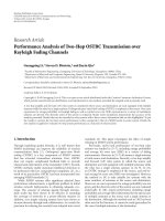
Figure 6 shows an example application workload model
—our case study—in an activity diagram. There are ten
execution tasks that are connected with edges that represent
channels between the tasks. Actions on the left column
(excluding the workload event) are tasks of the encoder,
whereas actions on the right column are tasks of the

decoder. Tagged values indicating integer operations and
send amounts are shown for each task. Other tagged values
have been left out from the figure for simplicity. The
trigger conditions for PreProcessing and VLCDecoding are
defined so that they execute the operations in a loop.
For example, PreProcessing task fires output tokens Xres ∗
Y res/MBPixelSize times to the channels c2 and c11 when

data arrives from the incoming channel c1. This amount
corresponds to the number of macroblocks in a single
frame. Consecutive processing of this task is triggered by
the incoming data token from the loop channel c11. The
number of loop iterations for a single frame is thus the
same as the number of macroblocks in one frame (Xres ∗
Y res/MBPixelSize). The trigger conditions for other tasks
are defined so that they process the operations and send
data to next process when a data token is arrived to their
incoming channel. Send probability for all tasks and trigger
conditions is 1.0. In this case sent data amounts are defined as
expressions depending on the macroblock size, bits per pixel
(BPP) value, and image resolution. The operation counts
are set as constant values fixed for the utilized macroblock
size. There is also a single periodically triggered workload
event, that feeds the application workload network. Global
parameters used in expressions are defined in upper right
corner of the figure.
5.2. Platform Performance Model Presentation. The platform is modeled with stereotyped UML2 classes and class


10

EURASIP Journal on Embedded Systems
//quantization parameter (1-32)
$qp = 16
// frame rate (frames/s)
$fr = 35
// image size
$Xres = 352

$Yres = 240
// bits per pixel
$BPP = 12
$MBPixelSize = 256

<<WorkloadEvent>>
VideoInput
{eventKind = periodic,
sendAmount = “1”,
sendPropability = “1.0”,
time = “1.0/fr”}
c1
<<ExecutionWorkload>>
PreProcessing
{intOps = 56764,
sendAmount = “MBPixelSize∗BPP/8”}
(Encoder::)

<<ExecutionWorkload>>
MBtoFrame
{intOps = 5440,
sendAmount = “MBPixelSize∗BPP/8”}
(Decoder::)

c11

c10

c2

<<ExecutionWorkload>>
MotionCompensation
{intOps = 4222,
sendAmount = “MBPixelSize∗BPP/8”}
(Decoder::)

<<ExecutionWorkload>>
MotionEstimation
{intOps = 29231,
sendAmount = “MBPixelSize∗BPP/8”}
(Encoder::)
c3

c9
<<ExecutionWorkload>>
IDCT
{intOps = 15184,
sendAmount = “MBPixelSize∗BPP/8”}
(Decoder::)

<<ExecutionWorkload>>
DCT
{intOps = 13571,
sendAmount = “MBPixelSize∗BPP/8”}
(Encoder::)
c4

c8

<<ExecutionWorkload>>

Quantization
{intOps = 9694,
sendAmount = “MBPixelSize∗BPP/8”}
(Encoder::)

<<ExecutionWorkload>>
Rescaling
{intOps = 4938,
sendAmount = “MBPixelSize∗BPP/8”}
(Decoder::)

c5
<<ExecutionWorkload>>
VLC
{intOps = 11889,
sendAmount = “(Xres∗Yres∗BPP/8)
/(qp∗3)”}
(Encoder::)

c7

c6

<<ExecutionWorkload>>
VLDecoding
{intOps = 61576,
sendAmount = “MBPixelSize∗BPP/8”}
(Decoder::)

c12

Figure 6: Example workload model in an activity diagram.

instances. Other alternative would be to use stereotyped
UML nodes and node instances. Nodes and devices in
deployment diagrams are the native way in UML to model
coarse grained HW architecture that serves as the target
to SW artifacts. Memory and communication resource
modeling are not natively supported by UML2. Therefore,
MARTE hardware resource modeling (HRM) package is
utilized to classify different types of HW elements.
MARTE hardware resource modeling package offers
several stereotypes for modeling embedded HW platform.
The complete hardware resource model is divided into

logical and physical views. Logical view defines HW resources
according to their functional properties whereas physical
view defines their physical properties, such as area and power.
The performance modeling does not require considering
physical properties, and thus, only stereotypes related to the
logical view are enough for our needs. Next, the stereotypes
utilized from MARTE HRM to categorize different HW
elements are discussed in detail.
HW ComputingResource is a generic MARTE stereotype
that is used to represent elements in the HW platform which
can execute application functionality. It can be specialized


EURASIP Journal on Embedded Systems

11

<<metaclass>>
Element

<<stereotype>>
PePerformance
[Element]
+intOpsPerCycle: Real
+floatOpsPerCycle: Real
+memOpsPerCycle: Real
+opFreq: NFP_Frequency

<<stereotype>>
MemPerformance
[Element]
+rdOpsPerCycle: Real
+wrOpsPerCycle: Real
+opFreq: NFP_Frequency

<<stereotype>>
CommPerformance
[Element]
+txOpsPerCycle: Real
+opFreq: NFP_Frequency

Figure 7: Stereotype extensions for HW platform performance.

<<hwProcessor>>
<<PePerformance>>

<<ep_allocated>>
cpu1: ARM9
{opFreq = “150 MHz”}

<<hwProcessor>>
<<PePerformance>>
<<ep_allocated>>
cpu2: ARM9
{opFreq = “120 MHz”}

<<hwProcessor>>
<<PePerformance>>
<<ep_allocated>>
cpu3: ARM9
{opFreq = “120 MHz”}

hibi_p

hibi_p1

hibi_p

hibi_p3

hibi_p

<<hwBus>>
bus: Hibi_segment

hibi_p2

Figure 8: Execution platform performance model.

to, for example, HW Processor to indicate its properties as a
programmable computing resource. This stereotype or any
of its inherited stereotypes is used to represent processing
element pe ∈ PE.
HW Memory is a generic MARTE stereotype for resources that are capable of storing data. This stereotype
and its inherited stereotypes, such as HW RAM, are used to
represent storage element se ∈ SE.
Finally, generic MARTE stereotype HW CommunicationResource and its inherited stereotypes, such as HW Bus,
are used to represent communication element ce.
The performance related characteristics are given with
three additional stereotypes presented in Figure 7. The
PePerformance is applied for a processing resource, MemPerformance for a memory resource, and CommPerformance for
a communication resource, respectively. The performance
characteristics are given for the elements with tagged values
of the stereotypes that define the performance indices and
operating frequency of the particular elements.
Figure 8 presents an example platform model in a UML
composite structure diagram with performance characteristics. In the figure, there are three instances of HW processors
(UML parts) connected to a single bus segment with UML

ports and connectors. The shown tagged values indicate the
operating frequency of the processors.
5.3. Mapping Model Presentation. MARTE allocation package is used to model the mapping of application tasks onto
platform resources. MARTE allocation mechanism allows
hybrid allocation in which application behavioral elements
are associated with structural platform resources. The hybrid
allocation is performed with two stereotypes ApplicationAllocationEnd and ExecutionPlatformAllocationEnd. In UML

diagrams they are written as app allocated and ep allocated
for conciseness. Application allocation end has a tagged
value that describes the platform resources to which the
particular application element is mapped. Execution platform allocation end identifies the platform resources onto
which application elements can be mapped. A dependency
stereotyped Allocated is used to bind application behaviour
elements onto platform elements.
An example mapping with the MARTE allocation mechanism is shown in Figure 9. In the figure, the tasks defined
in the workload model of Figure 6 are mapped onto HW
processors defined in the HW platform model of Figure 8.


12

EURASIP Journal on Embedded Systems

<<app_allocated>>
PreProcessing

<<app_allocated>>
MotionEstimation

<<app_allocated>>
DCT
<<Allocated>>

<<Allocated>>

<<app_allocated>>
VLDecoding

<<app_allocated>>
Quantization
<<app_allocated>>
VLC
<<Allocated>>
<<Allocated>>

<<Allocated>>

<<app_allocated>>
IDCT
<<app_allocated>>
Rescaling

<<app_allocated>>
MBtoFrame

<<app_allocated>>
MotionCompensation

<<Allocated>>
<<Allocated>>
<<Allocated>>

<<Allocated>>
<<Allocated>>
<<ep_allocated>>
cpu1: ARM9

<<ep_allocated>>
cpu2: ARM9

<<ep_allocated>>
cpu3: ARM9

Figure 9: Mapping with MARTE allocation mechanism.

5.4. Parameterizing Models with MARTE VSL Expressions.
The MARTE value specification language (VSL) has been
developed to specify the values of constraints, properties
and stereotype attributes particularly for nonfunctional
properties. It is an extension to the Value specification and
DataType concepts provided by UML. It can be used in any
UML-based specification for extending the base expression
infrastructure provided by UML. The VSL addresses how to
specify variables, constants, and expressions in textual form.
It also deals with time values and assertions as well as how
to specify composite values such as collection, interval, and
tuples in UML models.
In our approach the syntax of VSL is utilized to define
expressions on application workload models and platform
performance models. It is an efficient way for parameterizing
the workload models according to application-related values.
Top-right corner of Figure 6 shows an example of using
VSL syntax to parameterize application workload models
according to video quality metrics that are dependent on the
application. In the example, frame rate (fr) is set to 35 frames
per second and this constant variable is utilized to determine
the time period for the VideoInput workload event when

a single image is fed to the process network. Further, the
macroblock size in pixels (MBPixelSize) and image size (Xres
and Yres) are used to determine the data amounts transferred
between tasks.

6. Tool Framework for Model-Driven SoC
Performance Evaluation and Exploration
The presented performance evaluation models are used for
early analysis of data intensive embedded systems. Figure 10
presents the tool framework in which the models are applied.
6.1. Performance Model Capture and System-Level Simulation.
The flow begins from capturing the system performance
modeling in UML2 using the presented model elements and
profiles. This is followed by the model parsing phase in which
the models are transformed into XML system model (XSM)
[24, 25]. This is the corresponding XML presentation of the
UML2 performance models. The XSM is a common format
between tools to exchange information on the designed
system. The XSM can be modified by tools after its creation
during the design-space exploration iterations.

UML2 performance model

Model parser

Back-annotator

XML system model
SystemC simulation with
transaction generator

Performance results
Design-space
exploration tool

Execution
monitor

Figure 10: Tool framework for performance evaluation and
exploration.

After model creation the XSM file is fed to the simulator.
The simulator is divided into two parts: computation and
communication. The computation part is in practice realized
with a configurable transaction generator (TG) [21]. The
computation part simulates the execution and scheduling
of tasks on processing and memory elements. It also
feeds the underlying communication part with data tokens
transmitted between tasks which are mapped onto different
platform elements. The abstraction level of the computation
part is the same with the metamodel defined in Section 3.
Due to high abstraction level of the computation part,
the executed tasks do not contain any specific functionality,
but they only reserve the processing or memory element and
block it from other tasks for certain amount of time. For
example, for execution tasks this time is derived with (17).
The computation part (TG) is configured automatically
based on the abstract task, processing and storage resource
models defined in UML. The configuration is based on
generating corresponding SystemC code containing the same
tasks, processing and memory elements. This is done by

instantiating generic task and HW element SystemC components with parameters (operation counts, performance
indices, etc.) defined in UML the models.
The computation and communication parts are interfaced with Open Core Protocol (OCP) [26] TL2 compatible


EURASIP Journal on Embedded Systems
Table 1: Summary of collected and monitored performance
statistics.
Category
Application
specific

Application

Values
For example, frame rate, radio
throughput

Task
communication

Signals in/out, avg./tot.
communication cycles,
communication % of execution
time, intra/inter-PE
communication bytes and cycles,
communication cycles/byte

Task general
Mapping

Execution count, avg./tot.
execution cycles, execution % of
thread/service total, signal queue,
execution latency, response time
Task to thread/PE

PE

Utilization, inter-PE
communication bytes, avg./tot.
execution cycles

Network

Platform

Utilization, efficiency

interfaces. This means that the communication part can
be changed to any SystemC-based network model that
implements OCP TL2 compatible interfaces for interconnected elements. This allows simulation of low abstraction
level models of communication (such as NoCs) with high
abstraction level models of computation. Currently, the
earlier presented simple performance model for communication element is not used in our framework. Instead,
a more accurate SystemC defined TLM model for the
communication part is used in simulations.
6.2. Execution Monitoring. After simulation the simulator
tool produces a performance result file. It is a detailed
description of events of particular interest during simulation.

This file can be used as an input to Execution Monitor [27]
program that can be used to visualize the simulation in
a repeatable manner. The collected and monitored performance statistics are summarized in Table 1. The monitoring
of simulation is efficient in spotting trends, correlations, and
anomalities in system performance over time. In addition, it
is efficient in understanding dynamic effects such as varying
delays (jitter) and race conditions due to contention and
scheduling.
Performance bottlenecks can be detected by observing
the amount of tokens in signal queues and the utilization
of PEs. If the number of tokens in the incoming channel
of a task is increasing it is usually an indication of that task
being the bottleneck in a chain of several tasks. On the other
hand, a bottleneck can be located when a single processor
has a considerably higher utilization than other collaborating
processors.
In practice, the modeled response time requirements are
validated by observing the maximum response time of a
task in different execution scenarios. Meeting throughput
requirements can be also observed in a similar manner.

13
Figure 11 presents the control view of the execution
monitor tool. In the figure, the control view shows a system
consisting of ten tasks mapped onto three processors. Each
processor column consists of the current task mapping on
top and an optional graph on the bottom. The graph can
present, for example, processor utilization as in the figure.
6.3. Design-Space Exploration. After simulation and performance monitoring, the performance simulation results and
XSM are fed to the design-space exploration tool which

tries to optimize the platform parameters and task mapping
so that user-defined cost function is minimized. The cost
function can contain several nonfunctional properties such
as power, frequency, area, or response time of an individual
task. The design space exploration tool has several mapping
heuristics supported: simulated annealing, group migration,
hybrid of the previous two [28], optimal subset mapping
[29], genetic algorithm, and random. The design-space
exploration cycle continues by performing the simulation
after each remapping or modification in the execution
platform.
After the design-space exploration cycle ends, the optimized system description is again written to the XSM file.
The back-annotator tool is used to change the UML2 models
according to the results of the design-space exploration
(updated platform and mapping).
6.4. Governing the Tool Flow Execution. The execution of the
design flow is governed by a customizable Java-based tool
for configuring and executing SoC design flows. This tool
is called Koski Graphical User Interface. The idea of this tool
is that a user selects tools to the flow to be executed from
a library of tools. New tools can be imported to the library
in a plug-and-play fashion. Each tool includes a section of
XML which specifies the input and output tokens (files and
parameters) of that particular tool. Parameters of individual
tools can be set via the GUI. For example, the platform
constraints such as maximum and minimum number of PEs
and the cost function of the design-space exploration tool
are these kind of parameters. Due to its flexibility, this tool
has shown to be very effective in researching and evaluating
different methodologies and tool flow configurations.

7. Case Study: Performance Evaluation
and Exploration of a Video Codec on
Multiprocessor SoC
This section presents a case study that illustrates the applicability of the modeling methods and tool framework in
practice. The application is a video codec on a multiprocessor
platform. We used an approach in which new functionality
representing web client was modeled and added to an
existing video codec system in Figure 6 and the system
was simulated and optimized based on the monitored
information.
7.1. Profiling and Modeling. All the functions were modeled
by their workload and simulated in SystemC using TG. The


14

EURASIP Journal on Embedded Systems

100

Processor utilization

100

Processor utilization

100

75

75

50

50

50

25

25

25

0

0

Processor utilization

75

100 110 120 130 140 150 160 170 180 190

0
100 110 120 130 140 150 160 170 180 190

100 110 120 130 140 150 160 170 180 190

Figure 11: Control view in execution monitor.

workload model of the video codec was originally profiled
from real FPGA execution trace whereas the model of the
web client was only a single task which had an early estimate
of its behavior.
The performance requirement of the video codec was
set to 35 frames per second (FPS). Thus, an external
event representing the camera triggered at 35 Hz frequency.
The HW platform consisted of three processors connected
through a shared bus. The operating frequencies of the
processors were set to 150 MHz, 120 MHz, and 120 MHz.
The frequency of the bus was set to 100 MHz.
7.2. Simulating and Monitoring. When the original system
was simulated, it was observed that it met the FPS requirement. Next, functionality for the web client was added to
run in parallel with the video codec. The web client was
mapped to cpu1 (see Figure 11) because it was observed that
the utilization of cpu1 was the lowest in the original system.
Simulations indicated that the performance of the video
codec was decreased to 14 FPS. In addition, cpu1 became
fully utilized at all times whereas the utilizations of the other
two processors decreased. This indicated a clear bottleneck
on cpu1 as it was not able to forward processed data fast
enough to other processors. This could also be observed
from the signal queues of the tasks mapped onto cpu1. The
environment produced raw frames so fast that they started
accumulating at the cpu1.
Thereafter, a remapping of the application tasks was
performed since the workload of the processors was clearly
imbalanced. The mapping was done manually so that all the

encoder tasks were mapped to cpu1, the decoder tasks to
cpu2, and the web client functionality was isolated to cpu3.
During the simulation it was observed that this improved the
FPS to 22.
Because the manual mapping did not result in the
required performance, the next phase was automatic

exploration of the task mapping. The result mapping was
nonobvious because the tasks of the encoder and decoder
were distributed among all the processors. Hence, it is
unlikely that we had ended to it with manual mapping.
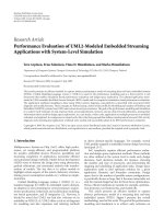
The system became more balanced and the video codec
performance increased to 30 FPS, but it did still not meet the
required 35 FPS. Cpu1 was still the bottleneck and the signal
queues of the tasks mapped to it kept increasing. However,
they were not increasing as fast as with the unoptimized
mapping, as presented in Figure 12. Figure 12(a) illustrates
the queue before the mapping exploration and Figure 12(b)
after the exploration. The signal queues are shown for the
time frame of 50 to 100 ms, and the scale of the y-axis is 0–
150 signals.
Finally, automated exploration was performed for the
operating frequencies of the processors. The result of the
exploration was that the frequency of cpu1 was increased
40 MHz to 190 MHz, and the frequencies of the other
two processors were increased 20 MHz to 140 MHz. The
simulation on this system model showed that the FPS
requirement should be met, and the tasks could process all
the signals which they received.

8. Discussion
In early performance evaluation, the key issue is the tradeoff
between accuracy and development time of the model. The
best accuracy is achieved from cycle-accurate simulations
or from actual implementation. However, constructing the
cycle-accurate model or integrating the system is very time
consuming in comparison to using system-level models
and simulations. Thus, utilization of abstract system-level
models allow the designer to explore the design space
more efficiently. The actual simulation time is also faster
in system-level simulations in comparison to cycle-accurate
simulations.


EURASIP Journal on Embedded Systems

15

VLC: Signal queue

150

VLC: Signal queue

150

125

125

100

100

75

75

50

50

25

25
0

0
50

55

60

65

70

75

80

85

90

95

(a) Before mapping exploration

50

55

60

65

70

75

80

85

90

95 100

(b) After mapping exploration

Figure 12: Signal queues for task VLC before and after mapping exploration.

In this work we concentrate on reducing the effort
in specifying and managing the performance models for
system-level simulations. This has been done by utilizing
graphical UML2 models. As a result, the degree of readability
of the models is improved in comparison to textual presentation. The case study showed that the system model is easy
to construct, interpret, and modify with the presented UML
model elements. The case study models were constructed
in few hours. Profiling and estimating operation counts for
workload tasks can be considered time-consuming and hard.
In our case, it was done by profiling similar application
executing on FPGA.
MARTE VSL was found useful for defining expressions. It
significantly simplified modifying the models with different
application-specific parameters in comparison to using
constant values.
In earlier study [30] the average error in frame-rate was
4.3%. This article uses the same metamodel. Hence, it can
be concluded that our method offers designer-friendly, rapid
yet rather accurate performance evaluation for RTES.

9. Conclusions and Future Work
This article presented an efficient method to model and
evaluate streaming data embedded system performance with
UML2 and system-level simulations. The modeling methods
were successfully utilized in a tool framework for early
performance evaluation and design-space exploration. The

case study showed that UML2, the presented modeling
methods, and the utilized performance evaluation tools
form a designer-friendly, rapid yet rather accurate way of
modeling and evaluating RTES performance before actual
implementation. Future work consists of taking account
the impact of SW platform in the RTES performance
metamodel. This includes the workload of SW platform
services (such as file access and memory allocation) as well
as scheduling of tasks with different policies.

References
[1] Object Management Group (OMG), “Unified Modeling Language (UML) Superstructure,” V2.1.2, November 2007.
[2] G. Martin and W. Mueller, Eds., UML for SOC Design,
Springer, 2005.
[3] K. Berkenkă tter, Using UML 2.0 in real-time development
o
a critical review,” in International Workshop on SVERTS:
Specification and Validation of UML Models for Real Time and
Embedded Systems, October 2003.
[4] R. B. France, S. Ghosh, T. Dinh-Trong, and A. Solberg,
“Model-driven development using UML 2.0: promises and
pitfalls,” IEEE Computer, vol. 39, no. 2, pp. 59–66, 2006.
[5] Object Management Group (OMG), “A UML profile for
MARTE, beta 1 specification,” August 2007.
[6] Object Management Group (OMG), “OMG systems modeling
language (SysML) specification,” September 2007.
[7] P. Kukkala, J. Riihimă ki, M. Hă nnikă inen, T. D. Hă mă lă inen,
a
a
a

a aa
and K. Kronlă f, UML 2.0 profile for embedded system
o
design,” in Proceedings of the Conference on Design, Automation
and Test in Europe (DATE ’05), vol. 2, pp. 710–715, March
2005.
[8] M. Gries, “Methods for evaluating and covering the design
space during early design development,” Integration, the VLSI
Journal, vol. 38, no. 2, pp. 131–183, 2004.
[9] G. Kahn, “The semantics of a simple language for parallel programming,” in Proceedings of the IFIP Congress on Information
Processing, August 1974.
[10] Object Management Group (OMG), “UML profile for schedulability, performance, and time specification (Version 1.1),”
January 2005.
[11] T. Arpinen, M. Setă lă , P. Kukkala, et al., “Modeling embedded
aa
Ssoftware platforms with a UML profile,” in Proceedings of
the Forum on Specification & Design Languages (FDL ’07),
Barcelona, Spain, April 2007.
[12] K. Keutzer, S. Malik, R. Newton, et al., “System-level design:
orthogonalization of concerns and platform-based design,”
IEEE Transactions on Computer-Aided Design, vol. 19, no. 12,
pp. 1523–1543, 2000.
[13] G. Kotsis, Workload modeling for parallel processing systems,
Ph.D. thesis, University of Vienna, Vienna, Austria, 1995.


16
[14] P. Kukkala, M. Hă nnikă inen, and T. D. Hă mă lă inen, Pera
a
a aa

formance modeling and reporting for the UML 2.0 design
of embedded systems,” in Proceedings of the International
Symposium on System-on-Chip, pp. 50–53, November 2005.
[15] H. Hansson, M. Nolin, and T. Nolte, “Real-time in embedded
systems,” in Embedded Systems Handbook, chapter 2, CRC
Press Taylor & Francis, 2004.
[16] F. Boutekkouk, S. Bilavarn, M. Auguin, and M. Benmohammed, “UML profile for estimating application worst
case execution time on system-on-chip,” in Proceedings of
the International Symposium on System-on-Chip, pp. 1–6,
November 2008.
[17] C. Erbas, A. D. Pimentel, M. Thompson, and S. Polstra,
“A framework for system-level modeling and simulation
of embedded systems architectures,” EURASIP Journal of
Embedded Systems, vol. 2007, Article ID 82123, 11 pages, 2007.
[18] S. Balsamo and M. Marzolla, “Performance evaluation of
UML software architectures with multiclass queueing network
models,” in Proceedings of the 5th International Workshop on
Software and Performance, (WOSP ’05), pp. 37–42, July 2005.
[19] J. Kreku, M. Hoppari, T. Kestilă , et al., Combining UML2
a
application and SystemC platform modelling for performance
evaluation of real-time embedded systems,” EURASIP Journal
on Embedded Systems, 2008.
[20] G. Madl, N. Dutt, and S. Abdelwahed, “Performance estimation of distributed real-time embedded systems by discrete
event simulations,” in Proceedings of the 7th ACM & IEEE
International Conference on Embedded Software (EMSOFT
’07), pp. 183–192, 2007.
[21] T. Kangas, Methods and implementations for automated system
on chip architecture exploration, Ph.D. thesis, Tampere University of Technology, 2006.
[22] Object Management Group (OMG), “Meta object facility

(MOF) specification (version 1.4),” April 2002.
[23] Object Management Group (OMG), “Unified modeling language (UML) superstructure specification,” V2.1.2, November
2007.
[24] T. Kangas, J. Salminen, E. Kuusilinna, et al., “UML-based
multi-processor SoC design framework,” ACM TECS, vol. 5,
no. 2, pp. 281–320, 2006.
[25] E. Salminen, C. Grecu, T. D. Hă mă lă inen, and A. Ivanov,
a aa
“Networkon- chip benchmarking specifications part I: application modeling and hardware description,” v1.0, OCP-IP,
April 2008.
[26] “Open core protocol international partnership (OCP-IP),”
OCP specification 2.2., May 2008, .
[27] K. Holma, T. Arpinen, E. Salminen, M. Hă nnikă inen, and T.
a
a
D. Hă mă lă inen, Real-time execution monitoring on multia aa
processor system-on-chip, in Proceedings of the International
Symposium on System-on-Chip (SOC ’08), pp. 16, November
2008.
a
a aa
[28] H. Orsila, T. Kangas, M. Hă nnikă inen, and T. D. Hă mă lă inen,
a
Hybrid algorithm for mapping static task graphs on multiprocessor SoCs,” in Proceedings of the International Symposium
on System-on-Chip, pp. 146–150, November 2005.
[29] H. Orsila, E. Salminen, M. Hă nnikă inen, and T. D.
a
a
Hă mă lă inen, Optimal subset mapping and convergence
a aa

evaluation of mapping algorithms for distributing task graphs
on multiprocessor SoC,” in Proceedings of the International
Symposium on System-on-Chip, November 2007.
[30] K. Holma, M. Setă lă , E. Salminen, M. Hă nnikă inen, and T.
aa
a
a
D. Hă mă lă inen, Evaluating the model accuracy in automated
a aa
design space exploration,” Microprosessors and Microsystems,
vol. 32, no. 5-6, pp. 321–329, 2008.

EURASIP Journal on Embedded Systems