báo cáo hóa học:" Research Article Limited Feedback Multiuser MIMO Techniques for Time-Correlated Channels" pot

Hindawi Publishing Corporation
EURASIP Journal on Advances in Signal Processing
Volume 2009, Article ID 104950, 21 pages
doi:10.1155/2009/104950
Research Article
Limited Feedback Multiuser MIMO Techniques for
Time-Correlated Channels
Eduardo Zacar
´
ıas B, Stefan Werner, and Risto Wichman
Department of Signal Processing and Acoustics, Helsinki University of Technology, P.O. Box 3000, 02015 Helsinki, Finland
Correspondence should be addressed to Eduardo Zacar
´
ıas B, fi
Received 1 December 2008; Revised 28 April 2009; Accepted 8 July 2009
Recommended by Nihar Jindal
This work presents limited feedback schemes for closed-loop multiple-input multiple-output systems using frequency division
duplex. The proposed methods employ compact feedback messages in order to (a) feed back and track a complete frequency-
flat channel matrix, to be used as input to multiuser multiplexing methods designed for full channel side information (CSI) at the
transmitter, and (b) enable the receiver to command the transmit weight adaptation, in order to maximize the link reliability under
strong intercell interference. Simulations show that the channel feedback accuracy provided by the proposed algorithms produces
a negligible bit error probability (BEP) performance loss in low mobility scenarios compared to the full CSI performance, and that
the proposed interference rejection techniques can effectively exploit an estimate of the interference statistics in order to enable
multiple-stream communications under the permanent presence of intercell interference signals.
Copyright © 2009 Eduardo Zacar
´
ıas B et al. This is an open access article distributed under the Creative Commons Attribution
License, which permits unrestricted use, distribution, and reproduction in any medium, provided the original work is properly
cited.
1. Introduction
Wireless communications with multiple antennas at trans-

mitter and receiver ends have the potential of offering high
data rates and spectral efficiency. On one hand, the data rates
can be increased by transmitting several parallel streams. On
the other, interference rejection techniques can be employed
to enhance the link reliability, enabling communications
under high interference levels. This can lead to an increase
in the spectral efficiency of the system, for example, by
tightening the reuse of the frequency spectrum. Similarly,
multiuser multiplexing techniques can enable several users
to share the same frequency resource, which also leads to a
higher spectral efficiency of the system.
In order to realize the afore-mentioned benefits of
MIMO systems in a computationally efficient manner, low
computational complexity linear detectors may be employed
that exploit full or partial CSI at the transmitter. The way
in which the CSI is acquired depends on the system under
consideration. For systems employing frequency division
duplex (FDD), which are of interest here, the use of a
feedback channel per user is necessary. Three main uses of
the feedback channel can be found in literature. The first
pertains the adaptation of the transmit antenna weights,
commanded by the receiver. For example, single-user closed-
loop eigenbeamforming systems deal with the right singular
vectors of a channel matrix, either by feeding back a
quantized version or recursively tracking it, see, for example,
[1–6]. This type of feedback has typically considered only
structured (e.g., orthonormal) matrices. The second use is
intended to provide the transmitter with an approximation
of the channel matrix estimated by the receiver, which is
then used as an input to multiuser multiplexing algorithms

such as [7–9]. This type of feedback deals with unstructured
matrices and has not received much attention in literature.
The third type of feedback content, which is not treated, is
the transmission of channel quality indicators (CQIs) for the
purposes of multiuser scheduling. Recently published work
in this area and related references can be found in [10].
This article is divided in the following two major
sections.
(1) Closed-loop MIMO communications under strong
interference conditions, which falls within the first category,
but is different from the eigenbeamforming problem, whose
scope is limited to the channel right singular vectors. In
the proposed methods, the receiver informs the transmitter
2 EURASIP Journal on Advances in Signal Processing
of the transmit weights that maximize the link reliability,
conditioned on an estimate of the statistics of the noise-
plus-interference signals. The general case of an arbitrary
number of data streams is considered, and a specialized low
computational complexity solution for the single stream case
is also provided. Furthermore, the algorithms can employ
either orthogonal or nonorthogonal transmit beams.
(2) Channel feedback algorithms that allow the reliable
tracking of a complete frequency-flat channel matrix, which
falls into the second category, and the goal is to provide the
input to multiuser MIMO solutions designed for full CSI. To
avoid excessive signaling of channel parameters, we propose
channel feedback methods based on the principles of partial
update. That is, only a small part of the channel matrix is
updated at each feedback instant. Moreover, a static channel
convergence analysis has been provided for the basic building

block of the channel feedback algorithms.
High data rate transmissions in closed loop MIMO
systems with limited feedback have been extensively studied,
see, for example, [1, 2, 5]. However, these solutions do not
assume any external interfering signals, and are therefore
not suitable for interference limited scenarios. In this work,
we propose algorithms for multiple stream transmission and
intercell interference cancellation, using a low rate feedback
channel and a linear receiver. This constitutes an extension
of the classical IRC receiver [11, 12] to closed-loop MIMO
systems, and differs from open-loop MIMO-IRC schemes
such as [13], where no CSI is used. In the proposed algo-
rithms, the receiver employs the feedback channel to instruct
the transmitter on how to recursively adapt the beamforming
weights in order to maximize the link reliability in the
presence of intercell interference. The proposed tracking
solution exploits both transmit and receive diversity, and a
short-term estimate of the interference-plus-noise statistics.
More specifically, the signal to interference-plus-noise ratios
(SINRs) are computed for each stream, as a function of the
transmit weights. These rates can then be used to compute
a link performance metric and the weights can be adapted
to optimize its value, with the feedback message conveying
the weight update information to the transmitter. For the
purpose of illustration, we use the total uncoded conditional
BEP of the user as a link quality metric. The resulting
algorithm can operate with any symbol constellation for
which the uncoded performance of the detector is known.
We stress that the formulation extends easily to other SINR
to BEP mappings, including channel coding or laboratory

measurements of actual receiver implementations. Further-
more, the proposed closed-loop MIMO-IRC algorithms can
operate on streams with equal transmit power and equal bit
load, giving a similar performance per stream. This can ease
the design of the adaptive modulation and channel coding
layer, when compared to a system using eigenbeamforming,
where the gains per stream are intrinsically different due to
the eigenvalue spread of the channel.
The closed-loop MIMO-IRC solutions presented can
be implemented on both orthogonal and nonorthogonal
transmit beams. This is a system design choice and will
be reflected in the way that the precoding (beamforming)
matrix will be updated, upon arrival of the feedback
messages. For example, an orthogonal beamforming matrix
can be updated based on increments to the real-valued
angles that parameterize the matrix, while a nonorthogonal
matrix can be updated via premultiplication with a matrix
exponential. Orthogonal transmit beams have the advantage
that the total transmit power is the sum of the individual
beam powers, as opposed to the nonorthogonal beams case,
where the total power varies with the nonorthogonality. This
eases the dynamic range requirements of the power amplifier,
compared to the usage of nonorthogonal beams. The use of
orthonormal matrix decompositions to feed back or track
the right singular vectors (eigenbeams) of a channel matrix
has been considered in [1, 3, 4, 6]. In contrast, the MIMO-
IRC algorithms presented here do not feed back the channel
eigenbeams, but rather inform the transmitter of the weights
that optimize the link performance metric, conditioned on
the current channel and the estimate of the interference plus

noise covariance matrix. For the particular case of a single
user with only one data stream (single beam, single user
system), a low computational complexity update arises as
an extension of [5], where the update is based on a single
complex-valued Givens rotor, which sequentially visits all the
coordinate planes associated with the optimal beamformer.
In the second part of this article, channel feedback
methods are presented, which allow reliable tracking of
the complete channel matrix of a user, employing low rate
feedback channels. The CSI so acquired can then serve as
input to any MU-MIMO multiplexing solution designed for
full CSI, for example, [7–9]. This type of CSI is different from
that considered in eigenbeamforming algorithms [1, 4, 5],
where the main idea is to exploit the orthonormal structure
of the right singular matrix of the channel, to enable an
efficient representation. The feedback of the unstructured
channel is based on a single-bit tracking of the real and
imaginary parts of every element of the complex-valued
channel matrix, where each scalar is tracked with the single-
bit tracking structure presented in [14]. Despite the simplic-
ity of such solution, reserving two feedback bits for each
channel coefficient may be prohibitive. To further reduce the
feedback requirements, we propose an alternative approach
basedonpartialupdates,whereonlyareducednumber
of channel matrix elements are updated on each update
instance. In particular, we consider a simple sequential
strategy where the update proceeds taking groups from a
circular list, which is shown to be sufficient in scenarios
with moderate antenna array sizes and low fading rates.
When the number of antennas or the fading rate increases,

however, a more sophisticated selection rule to determine
which elements of the tracked matrix will be updated is
required. Thus, a selective or ranked partial-update approach
sacrifices some feedback bits in order to signal which matrix
elements are the most urgent to update. These partial update
principles have been previously employed to decrease the
computational complexity in adaptive filters [15, 16], and
to enable good tracking performance in low-rate closed-
loop eigenbeamforming [17, 18]. A further insight into
the channel feedback problem is given in an accessory
study, where a link to the closed-loop eigenbeamforming
algorithms is made. Indeed, by vectorizing the channel
EURASIP Journal on Advances in Signal Processing 3
matrix and normalizing the resulting vector, any method to
track the dominant eigenbeam of a channel can be used,
while the norm of the vector is tracked with a single bit
tracking structure from [14]. These methods, however, do
not outperform the proposed partial update methods in the
considered simulation campaign.
This paper is organized as follows. Section 2 provides
a description of the system model under consideration.
Section 3 describes a particular link performance metric
used for linear receivers. This formulation will be used to
optimize the transmission weights for the case of single-
user MIMO-IRC communications in Section 4. The channel
feedback algorithms are described in Section 5, where both
a sequential and selective partial update strategy will be
applied to the recursive tracking of the whole channel
matrix of a user. A static channel convergence analysis
for the building block of the proposed channel feedback

algorithmsisgiveninSection 5.4. Simulations are provided
in Section 6 and conclusions are given in Section 7.The
appendix summarizes the different alternatives for tracking
matrices and vectors employed throughout this work.
2. System Model
The system under consideration is illustrated in Figure 1
and consists of a multiuser MIMO system with N
t
transmit
antennas, and N
u
slowly moving users. Each user has N
r
antennas and a feedback channel carrying binary messages
of length n
b
, b
i
∈{0,1}
n
b
×1
with frequency f
b
= f
x
/L,where
f
x
is the symbol frequency and L  1.

The transmitter employs a fixed overall amount of N
b
beams, with one data stream per beam. Each user is allocated
N
bi
out of the N
b
streams, and its beamforming weights and
symbols are represented by W
i
∈ C
N
t
×N
bi
and x
i
∈ C
N
bi
×1
,
respectively. We assume that the symbols of each stream have
an average power P
≡ E{|x|
2
}. The overall beamforming or
linear precoding matrix contains all the per-user matrices as
W
= [W

1
···W
N
u
] ∈ C
N
t
×N
b
,whereN
b
=

i
N
bi
. Similarly,
all the per-user symbols constitute the symbol vector x
=
[x
T
1
···x
T
N
u
]
T
∈ C
N

b
×1
.
The receiver output of user i at symbol period k is
y
i
(
k
)
= H
i
(
k
)
W
i
(
l
)
x
i
(
k
)
+ n
i
(
k
)
,

n
i
(
k
)
= H
i
(
k
)
⎛
⎝

m
/
=i
W
m
(
l
)
x
m
(
k
)
⎞
⎠
+ ν
i

(
k
)
+
N
I

m=1
u
mi
(
k
)
,
k
=
(
l
− 1
)
L + s, s = 0, 1, , L − 1, l = 1, 2, ,
(1)
where H
i
(k) is the channel matrix between the transmitter
and user i, n
i
(k) includes the Gaussian thermal noise ν
i
(k)

with E
{ν
i
(k)ν
i
(k)
†
}=σ
2
I, N
I
intercell interfering signals
u
mi
received by user i, and the intracell interference from the
beams belonging to the other n
u
− 1users,andl denotes the
update instant of the weights.
Let the noise-plus-interference covariance matrices Q
i
be
defined as
Q
i
(
k, l
)
≡ E


n
i
(
k
)
n
†
i
(
k
)

=
P

m
/
=i
H
i
(
k
)
W
m
(
l
)
W
†

m
(
l
)
H
†
i
(
k
)
+
N
I

q=1
E

u
qi
(
k
)
u
†
qi
(
k
)

+ σ

2
i
I.
(2)
As mentioned earlier, we assume that there are L symbol
periods, each representing an instance of (1), before the
feedback message is transmitted. The feedback message b can
convey information about the update of the transmit weights
(single user case), or about the CSI of each user (multiuser
case). The L symbol periods constitute a slot and the delay of
the feedback message is neglected. We model the interfering
signals as complex Gaussian signals, with a fading rate not
necessarily equal to that of the user.
We consider linear receivers Ω
i
∈ C
N
r
×N
b
i
,uponwhich
each user computes the following quantity for detection:
z
i
(
k
)
= Ω
†

i
(
k
)
y
i
,
= T
i
(
k, l
)
x
i
(
k
)
+ n

i
(
k
)
,
T
i
(
k, l
)
= Ω

†
i
(
k
)
H
i
(
k
)
W
i
(
l
)
,
n

i
(
k
)
= Ω
†
i
(
k
)
n
i

(
k
)
,
(3)
where the user i receives N
b
i
independent data streams,
T
i
(k, l)andn

i
(k) define an equivalent linear system, and each
user can compute its receiver Ω
i
independently.
The receiver matrix Ω
i
is in general a function of H
i
, W
i
,
and Q
i
. For the multiuser case, there is coupling between the
matrices Q
i

and W due to the intracell interference. This does
not occur in the single-user case, where Q is merely due to
intercell interference.
Conditioned on
{H
i
}
N
u
i=1
,andgivenW and the receive
filters
{Ω
i
}
N
u
i=1
, the SINR for each stream of user i is obtained
from (3)and(2)as
ρ
ip
:=



T
i,pp




2

q
/
= p



T
i,pq



2
+ ω
†
i,p
Q
i
ω
i,p
,
p
= 1, , N
bi
, i = 1, , N
u
,
(4)

where T
i,pq
is the element p, q of matrix T
i
givenin(3), Q
i
is defined in (2), ω
i,p
is the column p of Ω
i
, and the term
ω
†
i,p
Q
i
ω
i,p
is the expected power of the filtered noise, for the
stream p of user i.
In this paper, we will use the following receiver structure,
referred to hereafter as the MIMO-IRC receiver:
Ω
i
:= Q
−1
i
H
i
W

i
,
(5)
which generalizes the classical IRC receive diversity combiner
[11, 12]. This classical combining filter can be viewed as a
receiver for the particular case N
t
= N
b
= N
u
= 1.
4 EURASIP Journal on Advances in Signal Processing
+
+
1
N
t
W
y
i
1
u
1i
H
i
b
i
x
N

t
×N
b
N
r
× N
t
N
r
N
bi
User

i/N
u
Tx
Linear
Rx,
streams
External
interf.
W
≡[W
1
··· ]
···
···
···
W
N

u
ν
iN
r
ν
i1
u
n
I
i
Figure 1: System model. A fixed transmitter equipped with N
t
antennas and N
u
mobile users under intercell interfering signals. Each user
has a limited-capacity feedback channel.
For the MIMO-IRC receiver (5), the matrix T
i
reduces to
T
i
= Ω
†
i
H
i
W
i
= W
†

i
H
†
i
Q
−1
i
H
i
W
i
.
(6)
Similarly, the covariance matrix of the filtered noise becomes
E

n

i
n
†
i

=
Ω
†
i
Q
i
Ω

i
= W
†
i
H
†
i
Q
−1
i
H
i
W
i
= T
i
. (7)
Therefore, the SINRs (4)forstreamp under the IRC receiver
can be written as
ρ
IRC
ip
=
T
2
i,pp

q
/
= p




T
i,pq



2
+ T
i,pp
,
p
= 1, , N
bi
, i = 1, , N
u
.
(8)
These ratios can be used to define a link quality measure
as a function of the transmit weights, given knowledge of
the channel matrices and noise statistics. In the single user
case, the receiver can acquire knowledge of H and Q,and
use the feedback channel to command the adaptation of
W to optimize its interference rejection capabilities. In the
multiuser case, on the other hand, the receivers employ
channel feedback methods to convey their matrices H
i
to the
transmitter, which in turn uses the link performance metric

to jointly determine all the per-user transmit weights. The
use of an SINR to BEP mapping as a link performance metric
is described in the following section, and channel feedback
methods are described in Section 5.
3. Transmit Weight Optimization for
Link Reliability
Adapting the transmit weights is a central part of closed-loop
MIMO and closed-loop MU-MIMO systems. The weights
typically optimize a link quality measure, given the channel
conditions and noise statistics. For single user systems with
linear receivers, the N
b
dominant right singular vectors of H
are of interest if the noise is spatially white. Indeed, when the
precoder is restricted to be an orthonormal matrix, it can be
shown that the precoder formed by these vectors optimizes
the mutual information, the SNR of the weakest stream
under the ZF receiver, and the trace of the MSE matrix under
the linear MMSE receiver [19]. For MU-MIMO systems, the
weights must optimize the simultaneous transmission of the
N
u
users. For example, the sum-MMSE for all the users can
be solved iteratively by the transmitter, assuming that it has
knowledge of the channel matrices and the noise covariance
matrices [7].
When the disturbance signals are not spatially white,
however, the optimal MIMO precoder becomes a function
of both the channel matrix and the covariance of the noise
plus interference signals. Consider, for example, the mutual

information for independent Gaussian source symbols and
Gaussian noise with covariance Q,givenH,andafixedW:
I
(
W
| H
)
= log
2




Q + P HWW
†
H
†





Q
−1



. (9)
For spatially uncorrelated noise with Q
= I

N
r
, P equals
the transmit SNR divided by the number of streams, and
the mutual information reduces to log
2
|I + P W
†
H
†
HW|,
which is maximized by diagonalizing H
†
H. In any other case,
using only the channel information to choose the precoder
is suboptimal. Note that Q is only available to the receiver,
which must compute and feed back the optimal matrix
W, instead of the channel eigenbeams. Since the size of
the matrix being fed back is the same, a properly designed
feedback method has the potential of conveying the optimal
precoder, without additional feedback requirements.
In this work, we will consider the optimization of the
SINRs under the IRC receiver, as given in (8). For N
u
=
N
b
= 1, optimizing the instantaneous SINR minimizes the
expected uncoded BEP and maximizes the ergodic capacity.
The optimal precoding vector can be easily solved by the

receiver upon H, Q,andefficient tracking algorithms can be
used to signal the precoder adaptation through the feedback
channel. This is the subject of Section 4.1.
For the more general case of N
b
> 1, the statistics of each
SINR determine the performance of the associated stream.
However, a scalar function of the SINRs is needed as link
EURASIP Journal on Advances in Signal Processing 5
quality metric for transmit weight adaptation. In the single
user case, general-purpose stochastic search techniques are
used in conjunction with an update rule of the transmit
weights, to define a closed-loop IRC-MIMO system. This is
described in Section 4.2. For the MU-MIMO case, the weight
optimization provides the means to assess the performance
of the channel feedback methods presented in Section 5.
Simulation results are provided in Section 6,whichquantify
the performance loss incurred by the system when using the
output of the channel feedback algorithms, instead of the
true channel matrices H
i
.
The link quality measure considered in this article is
computed upon multiple SINRs as the average conditional
BEP, over all the streams. It is straightforward, however, to
use other metrics such as mutual information or a weighted
MSE. This is possible in the single user case, because the
feedback mechanism presented in Section 4.2 can be used
with any link quality measure.
Consider the SINRs per stream defined in (4)andamap-

ping P
ip
(·) between the SINR and the BEP, which represents
the uncoded performance of the detector, depending on the
symbol constellation employed on the data stream p by user
i. The total conditional BEP across the data streams is a
weighted sum of the BEP of the data streams of the user,
depending on the bit load per stream:
P
(
i
)

W | H
1
, ,H
N
u

=

p
b
ip

k
b
ik
P
ip


ρ
ip
b
ip

,
(10)
where b
ip
is the number of bits per symbol on stream
p of user i and P
ip
(·) can be any suitable SINR to BEP
mapping, including laboratory measurements. For the sake
of simplicity, we present simulation results based on the
AWGN BEP approximations for M-QAM and M-PSK given
in [20].
Furthermore, the total conditional BEP for the system,
that is, the BEP across the streams of all the users, is the
weighted sum of the individual BEP of the users
P

W | H
1
, ,H
N
u

=


i

p
b
ip

p,i
b
ip
P
(
i
)

W | H
1
, ,H
N
u

,
(11)
where the BEP of user i from (10) weighs in the total BEP
according to the ratio of its bit load to the total number of
bits of the system. The total BEP of the system is therefore
afunctionofW, when conditioned on the channel matrices
and assuming that the statistics of the interference-plus-noise
can be estimated. Note that orthogonal training sequences
would be required in the MU-MIMO case, for the receivers to

estimate their covariance matrices Q
i
and form the optimal
combiners.
4. Interference Tolerant Closed-Loop
MIMO Communications
This section describes novel closed-loop MIMO transmis-
sion schemes that enable single user communications in
the presence of strong intercell interfering signals. Based on
the SINRs of each data stream from (4) and a link quality
measure defined upon the SINRs (as discussed in Section 3),
the receiver commands the transmit weight adaptation
through the feedback channel. Assuming that the receiver
can acquire knowledge of H and Q, the link performance
metric can be treated as a function of the transmit weights W.
For the case of a single data stream, the single SINR is used
as metric, and the optimal weight vector can be computed
in a simple manner. This enables the use of an efficient low-
complexity tracking scheme to convey the optimal W to the
transmitter, and is described in Section 4.1.ForN
b
> 1,
on the other hand, the optimal W needstobecomputed
iteratively, and a generic stochastic perturbation technique
defines the update through the limited feedback channel.
Furthermore, two update rules are considered, reflecting
different orthogonality constraints for W. This is the subject
of Section 4.2.
The following sections deal with the particular case of
N

u
= 1, and we will drop the associated index i from matrices
T
i
, Q
i
, H
i
, Ω
i
.
4.1. Efficient Single Beam Algorithm Based on Jacobi Rotations.
The performance of the single data stream N
b
= 1is
determined by the statistics of the instantaneous SINR. In
this section, we discuss the weight vector that maximizes
the SINR under the IRC filter, and feedback mechanisms
to enable the tracking of the optimal precoder at the
transmitter.
Given the MIMO channel matrix H and the transmit
weights W
≡ w, the equivalent channel at the receiver is a
SIMO channel:
h
≡ Hw.
(12)
Using the IRC combiner from (5), matrix T in (3)collapses
to a scalar and the SINR gain becomes
1

P
ρ
opt
= h
†
Q
−1
h = w
†

H
†
Q
−1
H

w
, (13)
which is the SINR of the optimal SIMO combiner in [12].
However, (13) shows that (1) the optimal weight vector
w is an eigenvector associated to the dominant eigenvalue
of H
†
Q
−1
H, and (2) the dominant eigenvector of H
†
H
produces ρ
≤ ρ

opt
, with equality only if Q = σ
2
I. This implies
that to optimize the SINR, the feedback mechanism must
track the dominant eigenvector of H
†
Q
−1
H, rather than the
dominant channel eigenbeam.
Let the eigenvalue decomposition of Q be U
Q
Λ
Q
U
†
Q
.The
optimal SINR can be written as
ρ
opt
= P

U
†
Q
h

†

Λ
−1
Q

U
†
Q
h

=
P
N
r

m=1



(U
†
Q
h)
m



2
λ
Q,m
. (14)

In the SIMO case, the channel U
†
Q
h is Gaussian, conditioned
on Q. Furthermore, the joint statistics of the eigenvalues λ
Q,m
can be computed, and the expected BEP can be written as
an iterated integral of the conditional BEP, where the first
integral is taken over the channels and the second over the
6 EURASIP Journal on Advances in Signal Processing
interferers. This approach has been explored in [11], where
bounds for the symbol error probability are derived under
the assumption of independent elements of h. In the MIMO
case, however, the transformed channel U
†
Q
h = U
†
Q
Hw is
not a linear combination of independent Gaussian variables
because w is the dominant eigenvector of H
†
Q
−1
H. This
complicates the extension of the approach in [11] to the
MIMO case. Furthermore, the exact PDF of ρ
opt
is difficult

to obtain even in the SIMO case. To assess the best possible
performance, we will compute an empirical PDF based on
samples of users and interfering channels. This will be used
as a reference for the performance of the feedback algorithms
presented in what follows.
Assuming that both the channel matrix and the interfer-
ence covariance matrix have some temporal autocorrelation,
the dominant eigenvector of H
†
Q
−1
H can be tracked at the
transmitter with the use of the feedback channel. This can be
accomplished, for example, by using the D-JAC algorithm [5]
to track the dominant eigenvector of the modified channel
correlation matrix
R
= H
†
Q
−1
H.
(15)
The D-JAC algorithm [5]cantrackN eigenvectors of
a generic Hermitian matrix R
∈ C
M×M
, with an update
based on a single complex-valued Givens rotor. This rotor is
associated to a coordinate plane that is chosen sequentially

among all the MN
− N(N +1)/2 possible planes. In this
case, we have M
= N
t
, N = N
b
= 1 and, therefore, N
t
− 1
planes are considered. The combination of the IRC receiver
with the D-JAC update operating upon H
†
Q
−1
H for N
b
= 1
will be referred to as the IRC- D-JAC algorithm. Each plane
is updated by one rotor, where the indices (p, q) defining the
location of cosine and sine elements of the Givens rotor are
taken circularly from the list
{(2, 1), (N
t
,1)}.
The application of one rotor in plane (p, q)isdefinedas
W
(
l +1
)

= Φ
(
l +1
)
W
0
,
Φ
(
l +1
)
= Φ
(
l
)
J
p,q
(
l
)
Φ
(
0
)
= I,
(16)
where J
p,q
is the complex-valued Givens rotor or Jacobi
transformation in plane (p, q)[21], computed upon the

matrix R and the auxiliary matrix Φ(l)asin[5], l denotes
the update instant, and W
0
contains the first left column of
the identity matrix.
Alternatively, the use of vector codebooks can also be
considered. Assuming that the interferers are independent
of a spatially white user channel, we hypothesize that the
optimal weight vector is isotropically distributed on the
unit hypersphere, as in the case of spatially white noise.
Then one can use, for example, a Grassmanian codebook
[22] to feed back the optimal vector nonrecursively. On
the other hand, the multiple beam algorithm presented
in the following section can also be applied to the single
beam case. However, the IRC- D-JAC algorithm has lower
computational complexity and can achieve near-optimal
performance at low mobile speeds (cf. Section 6), and is
therefore preferred.
4.2. Multiple Beam Algorithm. Consider a single user with
N
b
> 1 data streams and the IRC combiner of (5). Because
no other users are present, there is no intracell interference,
and therefore no coupling between the matrices Q and W.
The SINR of stream p follows directly from (8)andequals
ρ
IRC
p
=
T

2
pp
T
pp
+

q
/
= p



T
pq



2
,
(17)
where the terms T
pq
represent interference between the
streams. It can be seen that making T
= W
†
H
†
Q
−1

HW diag-
onal produces SINRs equal to the eigenvalues of H
†
Q
−1
H.
While this can be accomplished efficiently by using the
D-JAC algorithm to track the N
b
dominant eigenvectors
of H
†
Q
−1
H, it results in an SINR spread as large as
the eigenvalue spread of H
†
Q
−1
H. The SINR spread is
performance detrimental if the symbol constellations of the
streams are fixed and identical. This can be compensated
by choosing fixed constellations with different bit loads,
upon the statistics of the eigenvalues of H
†
Q
−1
H. Alterna-
tively, adaptive constellation switching can be used, at the
expense of additional feedback overhead and computational

complexity. This motivates the use of a link quality metric
that can balance the stream performance while employing a
single, fixed symbol constellation for all the streams.
However, (6)and(17) determine how the matrix W can
influence the effective SINR of each data stream, and there-
fore a link performance metric such as the total conditional
uncoded BEP from (10) or the mutual information from
(9). The goal of the algorithms presented in this section
is to convey the optimal W to the transmitter through the
feedback channel.
In order to allow the tracking of the optimal beamform-
ing matrix based on short feedback messages, a stochastic
perturbation search is performed based on the current
knowledge of H, Q and the current beamforming weights
W. The receiver tests 2
n
b
stochastic perturbations about the
current W and chooses the one giving the best value of the
cost function of choice, for example, the BEP across streams
(10). Then the index of the chosen matrix is fed back to the
transmitter, which updates W in the same way as the receiver.
Two update formulas are considered, depending on whether
or not the transmit beams are restricted to be orthogonal. In
both cases, the candidate generation is controlled by a step
size parameter μ>0.
The update of a tall orthonormal matrix W is done
by adding increments to the angles that parameterize the
matrix through a cascade of complex-valued Givens rotors,
as defined in (A.1). This defines the IRC-SCGAS algorithm,

which can be considered an extension of the Stochastic
Complex Givens-based search over the Angle Space (SCGAS)
algorithm [6]. Let θ(l) contain 2N
t
N
b
−N
b
(N
b
+1) real-valued
angles associated to the current value of the beamforming
matrix W, that is, W(l)
= M(θ(l)) from (A.1). In this
case, 2
n
b
−1
perturbations k
n
are generated as i.i.d. zero-mean
real-valued Gaussian vectors and 2
n
b
candidate matrices are
generated as

A
2n−1
= M(θ(l)+μk

n
), A
2n
= M(θ(l) − μk
n
)

2
n
b
−1
n=1
.
(18)
EURASIP Journal on Advances in Signal Processing 7
Let m
∗
∈{1, ,2
n
b
} be the index of the candidate matrix
giving the best value for the cost function. The update
proceeds as
W
(
l +1
)
= A
m
∗

,
θ
(
l +1
)
= M
−1
(
W
(
l +1
))
,
(19)
where the updated parameters are kept within their nominal
ranges by using the inverse mapping M
−1
. Because the
mapping M(
·) only involves Givens rotors, the resulting W
matrix is guaranteed to be orthonormal without explicitly
enforcing the constraint. Alternatively, the candidates can
be built based on left multiplication with unitary matrices.
These matrices can be computed as cascades of complex-
valued Givens rotors. This type of update has been used
in the single-bit Incremental Givens Rotations Eigenbeam-
forming (IGREB) algorithm [6]. Furthermore, the unitary
matrices can also be built as matrix exponential of skew-
Hermitian matrices [21]. This has been exploited for single-
bit eigenbeamforming in [23].

The update of a nonorthogonal W will be done by left-
multiplication with nounitary matrix exponential (expm)
and is referred to as IRC-EXPM. The receiver generates 2
n
b
−1
matrices K
n
∈ C
N
t
×N
t
with i.i.d. zero-mean circular Gaussian
entries. The 2
n
b
candidate matrices are then built as
⎧
⎨
⎩
A
2n−1
=




N
b



e
μK
n
W(l)


2
F
e
μK
n
W
(
l
)
,
A
2n
=




N
b


e

−μK
n
W(l)


2
F
e
−μK
n
W(l)
⎫
⎬
⎭
2
n
b
−1
n=1
,
(20)
where the scaling restricts the squared Frobenius norm
to N
b
and constrains the average transmit power, and
e
(·)
is the matrix exponential [21]. Note that due to the
nonorthogonality of the transmit beams, a higher peak-
to-average power ratio (PAPR) of the transmitted signal is

observed, compared to the case of the orthogonal beams. Let
m
∗
be the index of the chosen matrix, as in the IRC-SCGAS
algorithm. The update is then W(l +1)
= A
m
∗
.
As mentioned earlier, the matrices W produced in the
IRC-EXPM algorithm are not constrained to have orthonor-
mal columns, as those produced by IRC-SCGAS are. This
can have an impact to the performance, because there are
more degrees of freedom associated to the nonorthogonal
beams, which allows the IRC-EXPM algorithm to find better
solutions to the optimization of the total BEP from (10).
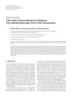
The performance difference is discussed in Section 6 and
illustrated in Figure 2.
4.3. Computational Complexity and Effect of the Fading
Rate. Recursive closed-loop MIMO algorithms can typically
achieve better tracking performance than the nonrecursive
solutions, over a range of low mobile speeds. The maxi-
mum speed up to which a recursive solution provides an
advantage is algorithm- and system-specific, and depends
on the convergence speed of the algorithm, the feedback
frequency, the fading rate of the channel, and also on
E
b
/N
0

(dB)
Average BER, 2 × 16QAM
IRC-SCGAS strong jammer
IRC-SCGAS noise dominated
IRC-EXPM strong jammer
IRC-EXPM noise dominated
Grassmanian CB 4
× 2 × 64
0510
10
−1
10
−2
10
−3
10
−4
10
−5
10
−6
15
Figure 2: MIMO-IRC algorithms in transmission of two data
streams, N
t
= 4, N
r
= 3, n
b
= 6 at 3 km/h. A strong jammer

situation with SNR at the receiver equal to that of the transmitter,
and one where the jammer has an SNR 30 dB below that of the user
(noise dominated scenario). Both orthogonal and nonorthogonal
transmit beams schemes are considered.
the operational SNR. Indeed, the errors associated to poor
tracking performance are less severe in low SNR conditions,
where noise and interference can partially mask the effects
of outdated transmit weights. Moreover, the optimal step
size also varies with the feedback rate and the mobile speed,
see, for example, [24] for an analysis of the performance of
signed stochastic gradient approximations in autoregressive
channel models. A performance comparison between the use
of static vector and matrix codebooks, and some recursive
eigenbeamforming solutions can be found, for example, in
[5, 17, 18].
Theuseofswitchedcodebooktechniquessuchas[2]or
hierarchical codebook structures such as the one described
in [25] could improve the performance of the systems
using static codebooks at low speeds. However, tuning the
associated adaptation parameters for different mobile speeds
can be time-consuming, and we have therefore restricted our
choice of alternatives to static codebook techniques.
Simulation results are provided in Section 6,which
illustrate the performance of the proposed algorithms under
a fixed feedback frequency, and as a function of the mobile
speed. In particular, it must be noted that the fading rate of
the gain matrix T in the equivalent system (3) is a function of
the relative motion speeds between transmitter and receiver,
and between the receiver and the interferers. It is expected
therefore that the performance degradation from increasing

the mobile speed is less severe if the relative motion between
the receiver and the interfering sources is slow. This can be
the case, for example, when a dominant interferer moves
8 EURASIP Journal on Advances in Signal Processing
roughly in the same direction of the receiver, with a similar
speed.
The single-beam algorithm IRC- D-JAC presented in
Section 4.1 offers a computational complexity reduction,
when compared to the cost of evaluating the optimal SINR
over a vector codebook of size 2
n
b
. Both algorithms require
computing R
= H
†
Q
−1
H. However, the codebook lookup
implies 2
n
b
evaluations of the quadratic form w
†
Rw,which
is O(N
2
t
), while the D-JAC has an update cost from (16), that
is, O(N

t
).
On the other hand, the multiple-beam algorithms
presented in Section 4.2 incur in a higher computational
complexity, when compared to the use of a fixed matrix
codebook. Both the codebook lookup and the stochastic
perturbations techniques require evaluating the cost func-
tion 2
n
b
times. However, generating the candidate matrices
from the current weights W is an additional cost associated
with the proposed algorithms. In the case of the IRC-
EXPM algorithm, this can be alleviated partially by using
precomputed matrix exponentials. In the case of the IRC-
SCGAS method, however, the cost of building the candidate
matrices from the perturbed angles cannot be avoided,
albeit the Givens rotations operations can be implemented
efficiently in hardware.
5. Limited Rate Channel Feedback
Methods for MU-MIMO
In this section, we consider recursive channel feedback
strategies for time correlated channels. These methods can
provide the transmitter with the user channel matrices
required by MU-MIMO solutions designed for full CSI, for
example, [7, 9, 26].
The proposed method is an alternative to predictive
vector quantization (PVQ) schemes like [27, 28], which
can have a high computational complexity due to vector
codebook lookup, codebook switching and the use of the

vector predictor. Furthermore, the associated codebooks
need to be trained for different mobility and channel
correlation assumptions. In contrast, we propose the use
of single-bit quantizers with adaptive step size, hereafter
referred to as “trackers,” to independently encode the real-
valued components of each channel element. This results in
a simplified design, which is shown to achieve good perfor-
mance in low mobility scenarios and moderate antenna array
sizes, with a low computational complexity (cf. Section 6).
Due to the limited-rate characteristic of the feedback
channel, the information about the trackers update must be
conveyed through messages of n
b
bits. This motivates the use
of partial updates, where a group of trackers is updated on
each slot. The ideas behind the tracker selection stem from
partial update adaptive filters [15, 16], and consist of both a
sequential partial update (e.g., round-robin update), and a
signal-dependent selective update, where a group of trackers
is selected for update, that gives the best improvement of a
given cost function. The single bit real-valued component
trackers (SBRVTs) consist of a memory device, which holds
the tracked value and the current value of the step size, and
a fixed rule for step size adaptation. The single-bit quantizers
are well-known components of linear and adaptive delta
modulation (ADM) signal representation techniques [29,
30], and the particular step size adaptation rule used here has
been considered earlier in variable step size LMS filters [14].
The SBRVT tracking structure and the assignment to
channel elements is described in the next section. Thereafter,

the round-robin and selective updates are formulated in
Sections 5.2 and 5.3, respectively. A convergence analysis
of the SBRVT in static channels is provided in Section 5.4,
where a bound of the expected convergence time is derived,
given the SBRVT parameters. Performance considerations
about the impact of the mobile speed are given in Section 5.5.
This section concludes with the formulation of an alternative
approach to the channel feedback problem, where a con-
nection to low feedback rate eigenbeamforming techniques
can be formed. The resulting methods are described in
Section 5.6.
5.1. Tracking Bas ed on Single-Bit Update for Real-Valued
Components. The proposed channel feedback algorithms use
atotalof2N
r
N
t
single-bit trackers, where each tracker fol-
lows a real-valued quantity defined as the real or imaginary
part of an element of the channel matrix. Depending on the
bit budget of n
b
bits and the update strategy, however, not
all the 2N
r
N
t
trackersmaybeupdatedonagivenfeedback
message. Let the real-valued components of the channel
coefficients be denoted by h

j
, j = 1 2N
t
N
r
and defined
as
h
j
=
⎧
⎨
⎩
Re
(
H
mn
)
j odd
Im
(
H
mn
)
j even
,
m
= 1+mod

j − 1

2

, N
r

,
n
= 1+

j − 1
2N
r

,
(21)
that is, the real and imaginary parts of H
mn
are listed
consecutively, and the enumeration proceeds along the rows
of H, from the leftmost to the rightmost column. A full
update will denote the feedback of 2N
r
N
t
bits, one for each
tracker. Depending on the antenna array sizes and fading
rates, a full update may not be necessary to enable good
tracking of H and partial updates can be considered, as
described in the following sections. We denote the tracked
value of h

j
as

h
j
.
The tracking function behind each

h
j
is defined as
follows. Let n
e
be the number of consecutive update bits with
the same sign that have occurred prior to the current update
instant. Similarly, let n
d
be the number of consecutive bits
with different sign. Additionally, the step size adaptation is
controlled by parameters Δ
min
, Δ
max
> 0 (bounds for the
step size Δ), α
u
> 1, 0 <α
d
< 1 (multiplicative factors
to vary the step size), and m

0
, m
1
, which are positive integers
controlling the responsiveness of the adaptation rule. Both
n
e
, n
d
are set to zero in the beginning, and the operation
proceeds as follows.
EURASIP Journal on Advances in Signal Processing 9
(1) Compute the current error
(l) = h(l) −

h(l),
with h(l) the true value of the channel component,
assumed known to the receiver.
(2) Examine the sign change counters: if sign[
(l)] equals
sign[
(l − 1)], increase n
e
by one and set n
d
to zero.
Otherwise, increase n
d
by one and set n
e

to zero.
(3) Apply the step size control: if n
e
≥ m
1
, then set Δ(l+1)
to max
{α
u
Δ(l), Δ
max
}. Otherwise, check if n
d
≥ m
0
.
If so, then set Δ(l +1)tomin
{α
d
Δ(n), Δ
min
}.
(4) Do the update: set

h(l+1)to

h(l)+sign[(l)]Δ(l +1).
Encode the binary decision sign[
(l)] in the feedback
message.

(5) Transmitter: upon receiving the feedback message,
extract the single bit associated to sign[
(n)].
(6) Transmitter: apply step size control for the transmit-
side step size Δ
tx
(l +1).
(7) Transmitter: reproduce the receive-side update by
setting

h
tx
(l +1)to

h
tx
(l) + sign[(l)]Δ
tx
(l +1).
As mentioned earlier, this tracking function is similar to
the continuously variable slope delta modulation techniques
from early speech digital transmission works [29, 30]. A
simplified version with Δ
min
= 0, Δ
max
=∞has been
used in [1] to track each of the angles parameterizing the
channel eigenbeams. We restrict our attention to the case
α

u
= 1/α
d
≡ α for simplicity. It will be shown in Section 5.4
that m
1
=α is a sufficient condition for convergence
in static channels. For tracking applications, however, the
parameters m
1
= m
0
= 1 can result in better performance
due to faster adaptation of the step size [14].
5.2. Sequential Update Channel Feedback. A simple partial-
update strategy updates groups of n
b
< 2N
r
N
t
trackers at
each update instance. No priority is given to any tracker, and
therefore all the trackers are visited sequentially in a circular
manner, n
b
trackers on each feedback message. Due to the
fixed update sequence, there is no need to include the indices
of the trackers to be updated, in the feedback message.
Let I represent the last tracker updated on the previous

slot. The update considers the n
b
trackers with indices
{1+(I + n)mod2N
r
N
t
}
n
b
−1
n
=0
. (22)
That is, the indices are visited circularly in groups of n
b
trackers, and the feedback message b contains the n
b
bits
destined to update the corresponding trackers.
Note that if n
b
is allowed to be larger than 2N
t
N
r
,
some trackers are visited more than once on a given update
instance, thus constituting a full update followed by a partial
update of n

b
− 2N
t
N
r
trackers. This resembles a step in data
reuse filtering [31], and can be necessary for fading rates
higher than those of pedestrian speeds (cf. Figure 3).
5.3. Ranked Partial-Update for SBRVT. As the dimensions
of the channel matrix grow, the selection rule for choosing
which trackers will be updated becomes important. Indeed,
due to the limited feedback characteristics of the system,
Empirical PDF
SBRVT 32 bits
SBRVT 40 bits
Givens, 6 rotors
Givens, 7 rotors
Givens, 8rotors
0
0.05
0.15
0.2
0
5
10
15
0.1
F
H − H
t


2
Figure 3: Tracking performance of channel feedback algorithms
for a system with N
t
= N
r
= 4 at 10 km/h. The partial update
alternative requires more than 40 bits to match the performance
obtained with 13 bits at 3 km/h (Figure 4). The Givens rotor-based
method for vectorized channels could improve the performance at
n
b
= 40 provided that 8 rotor angles can be encoded reliably. This
requires using (40
− 2)/16 ≈ 2.38 bits per angle, but the encoding
method is still an open problem.
a round-robin partial update may miss the trackers in the
most urgent need for update, which will translate to a poor
tracking performance. In this section, we describe a selective
partial-update method that can ameliorate this effect. Such
an approach employs part of the feedback message to
signal a group of trackers that should be updated next,
while the rest of the message contains the update bits for
the selected trackers. This ranked partial update strategy
has been applied before to closed-loop eigenbeamforming
algorithms in [17, 18] and is somewhat similar to the
antenna selection (AS) strategy for transmit diversity, albeit
AS requires only selecting which antennas are employed,
and does not transmit any information associated with the

selected antennas.
Consider a set
{c
n
∈{0, 1}
2N
t
N
r
×1
}
N
g
n=1
of binary vectors
with Hamming weight N
tr
representing N
g
different groups
of N
tr
trackers signaled for update. If a given vector c
m
is
chosen, then the trackers h
j
with index corresponding to the
nonzero entries of c
m

are to be updated. In order to ensure
that every tracker can be updated, the binary addition

n
c
n
must be a vector containing only ones.
The receiver tests each tracker group c
n
and ranks them
according to the total tracking error in the group, defined as
e
n
=
2N
t
N
r

m=1

h
m
−

h
m

2
δ


1, c
n,m

, n = 1, , N
g
,
(23)
where c
n,m
is the element m of c
n
,

h
m
is the current value
of the tracker associated to h
m
,andδ(·, ·) is one if both
arguments are equal, and zero otherwise.
10 EURASIP Journal on Advances in Signal Processing
Empirical probability density function
Perfect ranking reference
SBRVT 13 bits
Ranked SBRVT: 5 + 8 bits
0.02 0.04 0.06 0.08 0.1
0
10
20

30
40
F
H − H
t

2
Figure 4: Tracking performance of channel feedback algorithms
for a system with N
t
= N
r
= 4, n
b
= 13 at 3 km/h. The gain
from reserving 5 bits for signaling the elements selected for update
is shown. The reference for “perfect selection” has a very high
equivalent feedback requirement of n
b
= 24 + 8 = 32 bits.
The group with the largest error is then selected for
update. The feedback message contains n
b
bits, out of which
log
2
(N
g
) bits signal the chosen group, and the remaining
N

tr
bits contain the update information for each selected
tracker. This algorithm will be referred to as the ranked
single-bit per real-valued component tracking method (R-
SBRVT).
The choice of n
b
, N
tr
, N
g
such that n
b
= N
tr
+ log
2
N
g

is system-dependent and reflects a tradeoff between the
signaling overhead and the benefit of the ranked update. A
perfect ranking of the N
tr
most urgent trackers, on the other
hand, can result in an excessive overhead and is in general not
efficient. Such a scheme requires
log
2
(

2N
r
N
t
N
tr
)+N
tr
bits, and
it can be outperformed by the sequential algorithm operating
at the same feedback rate.
The problem of choosing the N
g
groups resembles a
vector quantization problem over a binary space of dimen-
sion 2N
r
N
t
. A thorough treatment of the problem is beyond
the scope of this article, and we have limited ourselves to
finding some groups of indices providing good performance,
throughnumericalsearchproceduresoversetsofN
g
binary
vectors of size 2N
r
N
t
with a “large” minimum Hamming

distance among them. As an example, Figure 4 shows the
benefit of the selective update in a system with n
b
= 13, N
t
=
4, N
r
= 4, where 5 bits are used to signal out one of N
g
= 32
binary vectors of Hamming weight 8, each representing a
group of trackers that can be updated.
5.4. Convergence of SBRVT in Static Channels. In this
section, we analyze the convergence properties of the SBRVT
mechanism described in Section 5.1. First, we model the
output of the tracker in response to a fixed input h,drawn
from a known distribution F
h
(·). Let

h(n) be the output of
the algorithm at update instant n. We say that the algorithm
converges to Δ
min
if there exists an integer v
t
> 0 such that
Δ(n)
= Δ

min
,foralln>v
t
. Without loss of generality, we
assume that h>0, and therefore the algorithm traces a
monotonically increasing curve until it surpasses the value
of h. The following three-branch function models the rise of
the algorithm output under a stream of positive input bits,
which is related to the aforementioned first segment of

h(·):
f
(
n
)
=
⎧
⎪
⎪
⎪
⎪
⎪
⎪
⎪
⎪
⎪
⎨
⎪
⎪
⎪

⎪
⎪
⎪
⎪
⎪
⎪
⎩
nΔ
min
, n ≤ m
1
,
m
1
Δ
min
+

1 −α
n−m
1
+1
1 −α
−1

Δ
min
, m
1
<n ≤m

1
+p,
f

m
1
+ p

+ Δ
max

n − p −m
1

, m
1
+ p<n,
p
=

ln

Δ
max
Δ
min

1
ln
(

α
)

.
(24)
We characterize the learning curve

h(·)byt monotonic
segments and t vertices, where a vertex is a pair v,

h(v)
defined as
sign


h
(
v − 1
)
−

h
(
v
)

=
sign



h
(
v +1
)
−

h
(
v
)

. (25)
In other words, the curve increases monotonically up to
the first vertex, after which the sign of the error changes
between vertices, up to vertex v
t
, after which the error
is bounded by Δ
min
. In the following, propositions will
summarize the results of the analysis. The proofs will be given
in Appendix B.
The following stablishes a sufficient condition for conver-
gence, assuming m
0
= 1.
Proposition 1. Given a static channel h,asufficient condition
for the SBRVT algor ithm to reach a vertex v
t
such that Δ(n>

v
t
) = Δ
min
is m
1
≤α, m
0
= 1,whereα ≡ α
u
= 1/α
d
.
Assuming the sufficient condition for convergence m
1
≤

α, m
0
= 1, the location of the first vertex can be computed
as follows.
Proposition 2. Given a static channel h and the conditions
m
1
≤α, m
0
= 1, the SBRVT algorithm reaches the first
vertex at the update time v
1
given by

v
1
=
⎧
⎪
⎪
⎪
⎪
⎪
⎪
⎪
⎪
⎪
⎪
⎪
⎪
⎨
⎪
⎪
⎪
⎪
⎪
⎪
⎪
⎪
⎪
⎪
⎪
⎪
⎩


h
Δ
min

, h ≤ m
1
Δ
min
,
m
1
+

ln

h −m
1
Δ
min
Δ
min
+1

×
(
α
− 1
)
+1


1
ln
(
α
)

, m
1
Δ
min
<h < f
(
Z
)
m
1
+ p +

h − f

m
1
+ p

Δ
max

, f
(

Z
)
<h,
(26)
EURASIP Journal on Advances in Signal Processing 11
where Z denotes m
1
+ p andwherethefunction f (·) and the
number p are given in (24).
Now, the number of vertices and their locations can be
determined. This gives the convergence time.
Proposition 3. The number of vertices t such that Δ(n>v
t
) =
Δ
min
is
t
=
⎧
⎪
⎪
⎪
⎪
⎪
⎨
⎪
⎪
⎪
⎪

⎪
⎩
1, h ≤ m
1
Δ
min
,
v
1
− m
1
, m
1
Δ
min
<h< f

m
1
+ p

,

ln

Δ
max
Δ
min


1
ln
(
α
)

, f

m
1
+ p

<h.
(27)
Furthermore, the vertices and their associated outputs are
v
i
=v
i−1
+

r
i−1
s

, r
i
=





r
i−1
−

r
i−1
s

s




, i=2, , t
r
1
:= f
(
v
1
)
− h, s = max

Δ
0
α
i−1
, Δ

min

,

h
(
v
i
)
= h +
(
−1
)
i+1
r
i
,
Δ
0
=
⎧
⎪
⎪
⎪
⎪
⎨
⎪
⎪
⎪
⎪

⎩
Δ
min
, h ≤ m
1
Δ
min
,
Δ
min
α
v
1
−m
1
, m
1
Δ
min
<h< f

m
1
+ p

,
Δ
max
, f


m
1
+ p

<h,
(28)
w ith v
1
computed from (26) and f (·), p defined in (24).
To conclude the analysis in static channels, we give an
upper-bound for the convergence time, and the expected
value of this bound, assuming that the cumulative distribu-
tion function (CDF) is known.
Proposition 4. The convergence time is upper-bounded by
N(h)
= 1+v
t
≤ 1+v
1
+α(t −1). Given a symmetric PDF of
h with CDF F
h
(·), the expected value of the convergence time
bound is given by

∞
−∞
N
(
x

)
f
h
(
x
)
dx
≤ 2
m
1

i=1
(
i +1
)
{F
h
[
iΔ
min
]
− F
h
[
(
i
− 1
)
Δ
min

]
}
+2
p

i=1
[
i
(
m
1
+1
)
+1
]
×

F
h

g
2
(
i
)

− F
h

g

2
(
i
− 1
)

+2

p +1

(
m
1
+1
)
+1

×

F
h

f

m
1
+ p

−
F

h

g
2

p

+2
∞

i=1

i + m
1

p +1

+ p +1

×

F
h

g
3
(
i
)


− F
h

g
3
(
i
− 1
)

,
g
2
(
i
)
= m
1
Δ
min
+
Δ
min
e
(i+1) log(α)
− αΔ
min
α −1
,
g

3
(
i
)
= iΔ
max
+ f

m
1
+ p

,
(29)
w ith the auxiliary function and number f (
·), p defined in
(24).
Note that the infinite summation term can be safely
truncated at a value i
max
such that F
h
[g
3
(i
max
)] ≈ 1.
Numerical examples of the expected convergence time are
given in Section 6.3.
5.5. Performance Of SBRVT in Time-Varying Channels.

When the channel component h is time-varying, the track-
ing error h(l)
−

h(l) becomes a random variable, and one
can attempt to compute its variance. One approach has
been proposed in [32], where the average error power from
tracking a linear segment h(n)
= nξ is averaged over the PDF
of the slope ξ. In particular, for Gaussian channels the slope
ξ is also Gaussian, and its variance can be computed from the
autocorrelation function, which in turn can be related to the
maximum Doppler frequency experienced by the receiver.
The study in [32] employed a simulations-based function
giving the average noise power for a given slope. Further-
more, the algorithm considered there was a discrete adaptive
delta modulation scheme, where the possible values of the
step size are a finite number of multiples of Δ
min
. On the
other hand, the slope approach of [32]canbeextendedto
the SBRVT case by using the formulation of the previous
section. Indeed, one can use the learning curve

h(n) =
f (n ≤ v
1
) to compute the average error in a linear segment.
However, the error so computed depends strongly on the
value assumed as initial step size, which in turn depends on

the state of the SBRVT previous to the entering the linear
segment. Thus, one needs to compute an expected initial step
size, and subsequently use it to average the error power over
the PDF of ξ. This calculation is complicated and beyond
the scope of this paper. We therefore restrict ourselves to
studying the performance of the sequential SBRVT-based
channel feedback method of Section 5.2, assuming that the
average error is known as a function of the mobile speed.
Let
e(v) be the average tracking error of the SBRVT
algorithm, for mobile speed v. The total average error for
i.i.d. variables h
i
is defined as
E
tot
=
2N
r
N
t

i=1
E


h
i
−


h
i

2

(30)
If using n
b
= 2N
t
N
r
feedback bits, every tracker is
updated on every slot, and each tracker has an update
frequency equal to the feedback frequency. More generally,
each tracker experiences an effective speed
v = 2N
r
N
t
v/n
b
,
and the total error is
E
tot
= 2N
t
N
r

e
(
v
)
, v = v
2N
t
N
r
n
b
.
(31)
This formula gives a rough prediction of the perfor-
mance, as shown in Figure 5.
12 EURASIP Journal on Advances in Signal Processing
Speed (km/h)
Av e ragesquared error
SBRVT reference
Simulation, 16 feedback bits
Simulation, 8 feedback bits
Prediction from (31), 8 feedback bits
10 20 30 50 60 70
0
0.5
1
1.5
2
2.5
3

3.5
40
Prediction from (31), 16 feedback bits
Figure 5: Performance of sequential channel feedback algorithm
for Nt
= 4, NR = 2 , as predicted from a single tracker simulations
with parameters Δ
min
= 0.001, Δ
max
= 0.6, m
0
= m
1
= 1, α = 1.1.
5.6. Methods B ased on Normalized Column Vectors. One of
the main considerations when comparing the feedback of the
whole matrix H with existing works in eigenbeamforming is
that the matrix H has no structure, its power is arbitrary, and
the columns are in general not orthogonal. In this section,
however, we show that both problems can be related.
Let

h = vec(H)/H
F
and n

h
=H
2

F
,wherevec(·)
converts the matrix argument to a single column vector
by stacking the columns vertically. Let n

h
befedbackto
the transmitter by using a single-bit tracking structure [14],
as any of the real-valued components h
j
of the previous
sections. It only remains to define how to track and feed back

h ∈ C
N
t
N
r
×1
, so that the transmitter can build its own version
of H,namely,H
t
.
We consider two alternatives for tracking

h,namely,(1)
build R
=

h


h
†
and use any closed-loop eigenbeamforming
algorithm to follow the dominant eigenvector, which is
trivially

h,and(2)treat

h as the N
b
= 1 case of the
matrix W and feed it back as in the IRC-EXPM algorithm
of Section 4.2,withcostfunction
||

h −

h
t
||
2
,where

h
t
is the
tracked version of

h.

Some eigenbeamforming algorithms like [5, 6]exploit
a phase ambiguity in the eigenbeams. This comes from the
fact that if v is an eigenvector of R,soise
jθ
v,whereθ is
an arbitrary angle. When using these algorithms, therefore,
a phase correction is required at the transmitter in order to
track

h. This angle can be tracked through a single bit tracker
and is computed as −arg(

h
†

h
t
).
As the product N
r
N
t
increases, the computational com-
plexity associated to updating

h by premultiplying with
matrix exponential also grows. Furthermore, the conver-
gence speed of a solution based on the D-JAC algorithm [5]
decreases with larger vector sizes, because the contribution of
each rotor to the overall change in the vector (after update)

becomes smaller. One possibility to escalate the algorithm
with the antenna array size or the fading rate is to increase
the number of coordinate planes per update to r>1rotors,
that is, to apply (16) r times per update. This, however,
poses a vector quantization problem, since all the 2r angles
associated to the rotors must be fed back to the transmitter.
The potential of this technique is illustrated in Figure 3,
where the updates proceed using unquantized rotor angles,
which constitutes the performance bound of the tracking
method.
6. Simulations
The simulation scenario consists of a transmitter with N
t
= 4
transmit antennas, and users moving at 3 km/h with a carrier
frequency of 2.1 [GHz], in spatially white Rayleigh fading
channels. Each slot contains L
= 160 symbols and has a
length of 1/1500 [s]. The interfering signals will be modeled
as Gaussian SIMO interferers, with a fading rate that is either
the same as that of the user, or is fixed at 3 km/h. A strong
jamming situation is considered, where a single interfering
signal arrives at the receiver with a signal-to-noise ratio equal
to that of the transmitter. It is assumed that each receiver
knows its channel matrix H
i
perfectly.
Whenever there is need to evaluate a conditional bit error
probability (BEP), we use the two-terms approximations
developed in [20] for M-QAM and M-PSK constellations.

The Gaussian Q function involved in the BEP expressions
can be evaluated with good accuracy with the approximation
[33].
6.1. Inter ference Tolerant Single User Communications. In
ordertoprovideafaircomparisonbetweenfeedbackmeth-
ods, and restrict the effect of the channel variations to limited
accuracy or limited convergence speed issues, we abstract
from the covariance matrix estimation problem. Therefore,
the algorithms will use a “near-perfect” estimate of Q(k, l),
given by

Q
i
(
k, l
)
= σ
2
i
I + u
1i
(
lL
)
u
†
1i
(
lL
)

.
(32)
In other words, the true covariance is computed at the
beginning of the slot l, and used throughout the L symbol
periods.
Figure 6 shows the average BER of the single beam
system, where 16QAM symbols are used, n
b
= 6 and the
mobile speeds are 3 km/h. It can be seen that the IRC-
DJAC reaches near-optimal performance. In comparison, the
eigenbeamforming (EBF) system employing an IRC receiver
suffers a penalty of several dB, because the interference
statistics are not considered for weight adaptation. Moreover,
the transmission without the IRC receiver is not feasible.
The empirical PDF of SINR achieved by IRC-DJAC is shown
in Figure 7 and compared to the SINR of the combination
EBF/IRC. The BER for the Grassmanian codebook of size 64
EURASIP Journal on Advances in Signal Processing 13
BEP, 16QAM
IRC-SCGAS μ = 0.15
IRC-DJAC 3 + 3
EBF + IRC
EBF + MF
EBF, no interference
Optimal SINR
Grassmanian CB
E
b
/N

0
(dB)
0510
15
10
−2
10
−4
10
−6
Single user, single beam system
Permanent interfering signal
Figure 6: MIMO-IRC algorithms under permanent intercell inter-
fering signal. Single beam system with N
t
= 4,N
r
= 2,n
b
= 6,
mobile and interfering signals at 3 km/h.
SINR (dB)
Empirical PDF
EBF/IRC
IRC-DJAC
IRC-DJAC
EBF/IRC
IRC-DJAC
EBF-IRC
10 15

20
25
30
5
0
0.05
0.1
0.15
Figure 7: Empirical PDF of SINR in N
t
= 4, N
r
= 2 single beam
system under a strong interfering signal, for E
b
/N
0
values of 0, 8,
16 dB and 4 bits per channel use. The IRC-DJAC uses 6 feedback
bits per slot. Its performance is compared to an unquantized
eigenbeamformer, used in conjunction with an IRC receiver. The
relative speeds Tx-Rx are identical to the relative speed interferer-
Rx, and equal to 3 km/h.
is also shown in Figure 6,whereadifference of about 1 dB to
the optimum is observed, at BER levels of 0.001.
The BER performance as function of the mobile speed is
given in Figure 8. As discussed in Section 4.3, if the relative
speed between the interferer and the receiver is small, then
some slowness is retained, which yields a better tracking
performance, compared to the case when the relative motion

Tx-Rx relative speed
IRC-MIMO single beam, 6 feedback bits
0dB,CB
6 dB, CB
10 dB, CB
6 dB, IRC-DJAC
0dB,IRC-DJAC
10 dB, IRC-DJAC
020304010
Average BER, 16QAM
10
−2
10
−1
10
−3
10
−4
Figure 8: Impact of the mobile speeds on the performance of the
single beam IRC-MIMO algorithm, using 6 feedback bits per slot.
Solid curves represent scenarios where the relative speeds Tx-Rx are
identical to the relative speed interferer-Rx. Dashed curves represent
scenarios where the interferer-Rx relative speed is fixed at 3 km/h.
between interferer and receiver is comparable to that between
the transmitter and the receiver. It can be observed that the
recursive techniques provide a performance advantage over
the range 3–30 or 3–20 km/h, depending on the SNR.
On the other hand, when two parallel streams are used,
a third receive antenna is necessary to cope with a single
interferer. In general, the IRC algorithm requires diversity

in order to cancel interference, so the requirement will be
N
r
>N
b
.
Figure 2 shows the performance of the IRC-SCGAS and
IRC-EXPM algorithms with two beams and 2
× 16QAM
constellations. The performance of the fully jammed (the
interferer has the same transmit power to noise power as
the user) is shown to be feasible, and a loss of 4 dB at
BEP 0.01 is observed, compared to the noise dominated
scenario. Based on the results of Figure 2, it is clear that the
transmission without the IRC receiver would be unfeasible.
The nonorthogonal beams provided by the IRC-EXPM
algorithm are shown to outperform the orthogonal beam
configuration, and the Grassmanian codebook of size 64
from [19] performs comparatively poorly. To be fair, this
codebook is meant for precoding in uncorrelated MIMO
channels under the assumption of spatially white noise, and
therefore the result presented here does not reflect negatively
upon the codebook methodology.
Figure 9 shows the trade-off between the number of
feedback bits for the IRC-SCGAS algorithm and its BEP
performance. It can be seen that the algorithm is able
to exploit additional receive diversity to further boost the
performance.
The distributions of the instantaneous rates log
2

(1 + ρ
i
)
are shown in Figure 10, for the limited mobility scenario of
3 km/h for both transmitter-receiver and interferer-receiver
channels. It can be seen that both streams have identical
statistics. The average of the instantaneous rate log
2
(1 + ρ)
is shown in Figure 11 for both streams.
14 EURASIP Journal on Advances in Signal Processing
E
b
/N
0
(dB)
Average BER, 2 × 16QAM
10
−1
10
−2
10
−3
10
−4
10
−5
MIMO IRC, two streams
Feedback bits per slot v/s performance
n

bψ
= 1
n
bψ
= 2
n
bψ
= 4
n
bψ
= 6
2
4
6
8 10 12 14 16
Figure 9: MIMO-IRC algorithms with two data streams and
orthonormal transmit beams. The tradeoff between feedback bits
per slot and uncoded average BER performance is shown for a
system with N
t
= N
r
= 4.
log (1 + ρ)
Empirical CDF
EBF/IRC
IRC-expm
0468 10
0
0.2

0.4
0.6
0.8
1
2
Figure 10: Empirical distribution of the instantaneous rates
log
2
(1+ρ
i
) for two data streams and a permanent interferer, at E
b
/N
0
values of 2, 8 and 14 dB. The IRC-EXPM uses n
b
= 6 feedback bits
and step size 0.05. The EBF/IRC system employs the unquantized
eigenbeams and an IRC receiver, but it does not take into account
the interference statistics. Both beams have the same statistics.
The sensitivity of the IRC-EXPM algorithm to the step
size parameter μ is illustrated in Figure 12, and it is shown
to depend on the SNR conditions. Finally, the performance
degradation as a function of the speed is given in Figure 13.
This degradation is also SNR-dependent, with smaller losses
at lower SNR.
6.2. Effect of the Channel Feedback Accuracy in Multiuser
Multiplexing. Figure 14 shows the performance of the BEP-
based solution with orthonormal precoders based on the
Average instantaneous rate

Stream 1
Stream 2
246
10
12
4
4.5
5
5.5
6
6.5
7
7.5
8 14
E
b
/N
0
(dB)
Figure 11: Ergodic capacity of each data stream for the IRC-Expm
algorithm using 6 feedback bits per slot. The relative speeds Tx-Rx
are identical to the relative speed interferer-Rx, and equal to 3 km/h.
The step size is 0.05.
Convergence step
BER performance of IRC-expm, 2 beams
4 dB
8 dB
12 dB
0.1 0.20.050
0.15

BER, 2 × 16QAM
10
−1
10
−2
10
−3
10
−4
Figure 12: Impact of the convergence step on the performance of
the IRC-EXPM algorithm with 2 data streams and a permanent
interferer. Both Tx-Rx and interferer-Rx speeds assumed 3 km/h.
parameterization of tall matrices (A.1). In order to update W,
the transmitter minimizes the BEP (11) by iterating over the
angle space with the random walk with direction exploitation
technique [34]. The well-known block diagonalization (BD)
technique [9] has also been considered. The BD uses a
factorized W: one factor eliminates the interference between
users, and the other implements eigenbeamforming on the
modified channel. For the BEP-based solution, it is assumed
that the transmitter broadcasts the optimal combiners. Alter-
natively, orthogonal training sequences could be used for
EURASIP Journal on Advances in Signal Processing 15
Speed (km/h)
4 dB
8 dB
12 dB
4 dB Interf-Rx 3 km/h
8 dB Interf-Rx 3 km/h
12 dB Interf-Rx 3 km/h

0
5
10 252015
30
BER, 2 × 16QAM
10
−1
10
−2
10
−3
10
−4
Figure 13: Impact of the mobile speeds on the performance of
the IRC-EXPM algorithm with two data streams and a permanent
interferer. The relative speed interferer-receiver equals the abcissa
value, unless otherwise stated.
estimation. The performance loss due to accuracy limitation
of the channel feedback algorithms is shown to be small for
the uncoded BEP range up to 0.01. It can be also observed
that the impact of the inaccuracy of the channel feedback
algorithms is more relevant when operating at very low BEP
levels such as 0.0001. On the other hand, the minimum
BEP solution achieves a performance gain of about 2dB,
compared to the BD scheme. This advantage comes from
lifting the restriction of nulling the interference among
users, which is a common approach in other MU-MIMO
techniques, for example, [7].
6.3. Numerical Examples for the Analysis in Static Channels.
In this section, we apply the analysis given in Section 5.4,to

study the effect of the different parameters on the expected
convergence time. We assume a zero-mean Gaussian distri-
bution of h with variance 1/2, such as that of the real-valued
components of the Rayleigh channel.
6.3.1. Fixing Δ
min
. We fix the minimum step size to satisfy
an expected value of the relative maximum residual error
Δ
min
/|h|. By discarding channel samples such that |h| <h
min
,
the expected error is approximately
0.5E

Δ
min
|h|

≈

∞
h
min
Δ
min
x
f
h

(
x
)
dx
=
Δ
min
2
√
π
Γ

0, h
2
min

, (33)
where Γ(
·, ·) is the incomplete Gamma function. This gives
Δ
min
as
Δ
min
=
√
π
Γ

0, h

2
min


desired average error

.
(34)
10
−2
10
−4
(Tx power/total bit load)/average noise power (dB)
Overall BEP (2 ×16QAM)
Multiuser MIMO, effect of channel feedback
BD, perfect CSI
BD, SBRVT
IRC-orth, perfect CSI
IRC-orth SBRVT
BD, Expm
IRC-orth Expm
−5
0
5
10
Figure 14: Effect of the channel feedback algorithms in multiuser
MIMO with N
t
= 4andtwouserswithN
r

= 2 each, both moving
at 3 km/h and employing a single data stream with symbols from
a 16QAM constellation. Two multiuser multiplexing solutions are
considered: BD refers to block diagonalization [9], and “IRC-orth”
minimizes the total conditional BEP from (11) with orthonormal
beams. The average uncoded BER of both is shown, when using
different types of CSI: perfect, SBRVT from Section 5.2 and a
normalized vector-based method from Section 5.6 with incremental
rotations based on matrix exponentials.
For example, using h
min
= 10
−32
, the required values
of Δ
min
for1,5,and10%areapproximatelyΔ
min
=
0.00025, 0.00125,0.0025.
6.3.2. Influence of Δ
max
and α. Assuming m
0
= 1andm
1
=

α, the expected convergence time is a function of Δ
max

, α.
The expected upper-bound can be computed in closed form
from (29), where F
h
(x) = 0.5(1 + erf(x)) is the CDF of
the zero-mean Gaussian variable with variance 1/2. The
integrand for the expectation is in general not smooth for
the exact convergence time v
t
+ 1, as shown in Figure 15.
Figure 16 shows the different expected values of the
convergence time bound, as a function of Δ
max
and α.It
can be seen that the choice of α is the most critical of the
two. On the other hand, the sample average of the exact
convergence time v
t
+1computedfrom(28) for each sample
h is shown in Figure 17. By comparing Figures 16 and 17,we
can see that the average of the exact convergence time is more
sensitive to Δ
max
than the expected value of the bound. The
best Δ
max
from both figures is Δ
max
= 0.17. Using this value,
the convergence time as a function of α can be considered. As

shown in Figure 18, both the bound and the exact formula
give an optimal value of α
= 3, for the current choice of
Δ
min
, F
h
. It can be observed that both curves exhibit local
minima at α
= 2, 3.
In order to verify the validity of the exact convergence
time 1 + v
t
computed from (28), the histogram of the con-
vergence time is shown in Figure 19, where both convergence
16 EURASIP Journal on Advances in Signal Processing
Static channel PDF
∗
convergence time
h
00.51
2
4
6
8
10
12
14
16
1.5

Figure 15: Integrands for the expected convergence time calcula-
tion, in Gaussian-distributed static channels: using the bound (
◦),
and using the exact convergence time (+).
Expected value of convergence time bound
1.5 2 2.5
3
3.5
20
25
30
35
40
45
α
Figure 16: Expected value of the convergence time bound from
(29), for Δ
max
∈ [0.05, 0.5] and Δ
min
= 0.00025, under convergence
condition m
1
=α and m
0
= 1.
times from (28) and from the actual algorithm run have been
plotted. Additionally, the histogram for the bound of the
convergence time, as given in Proposition 4. Furthermore,
to quantify the tightness of the bound, the histogram of the

difference between the bound and the true convergence time
is shown in Figure 20.
6.4. Performance of the Channel Feedback Algorithms. The
accuracy of the channel feedback algorithms can be studied
by defining the error between the true channel matrix H and
the fed back channel matrix, H
t
as
 :=H −H
t

2
F
. (35)
The error can be characterized statistically for a given
scenario. For example, Figure 21 shows the empirical prob-
ability density function (PDF) of the errors for algorithms
Av e rageconvergence time
2 2.5 3 3.5
22
24
26
28
30
32
34
α
Figure 17: Average value of the exact convergence time computed
by 1 + v
t

from (28), over 10
5
channel realizations. Curves are shown
for different values of Δ
max
∈ [0.05, 0.5] and Δ
min
= 0.00025, under
convergence condition m
1
=α and m
0
= 1.
Convergence time
Bound
Exact
1.5 2 2.5 3 3.5
25
30
35
40
45
50
55
α
Figure 18: Average value of the convergence time, for Δ
max
= 0.17
and Δ
min

= 0.00025, under convergence condition m
1
=α and
m
0
= 1. The expected value of the bound is computed according to
Proposition 4, and the exact time is computed from (28), averaged
over 10
5
channel realizations.
operating at n
b
= 7forN
t
= 4, N
r
= 2. It is shown that
a the sequential partial-update S-SBRVT outperforms the
methods based on vectorized channels from Section 5.6 (pre-
multiplication with matrix exponential and single Givens
rotor update). Given the small number of bits in the feedback
message, there is no gain to be achieved from the ranked
partial update concept. On the other hand, the impact
of
 to the BEP performance is shown in Figure 14,for
MU-MIMO solutions computed upon the output of S-
SBRVT and a vectorized channel with matrix exponential
premultiplication. The BEP performance due to the channel
EURASIP Journal on Advances in Signal Processing 17
Convergence time

Frequency
Predicted avg. is 21.94
Algorithm run. avg. is 21.94
Bound. avg. is 26.77
0
10
20
30
50
0
0.05
0.1
0.15
0.2
40
Figure 19: Convergence times from 10
5
Gaussian channel realiza-
tions. Δ
min
= 0.00025, Δ
max
= 0.17, α = 3, m
1
= 3, m
0
= 1.
The predicted convergence time 1 + v
t
from (28) is compared to

the true convergence time determined from running the algorithm.
Additionally, the bound for the convergence time 1 + v
1
+ α(t −1)
from Proposition 4 is also shown.
Histogram
Convergence time
0
2
4
6
8 10
12
0
0.5
1
1.5
2
2.5
Figure 20: Differences between the exact convergence time and
its upper bound, from Gaussian channel realizations. The average
difference is 4.479.
feedback methods is small in both cases, for levels of uncoded
BEP down to 0.01 (1%).
The use of predictive vector quantization (PVQ) [27]
can also be considered. However, choosing the classification
criteria for codebook selection and determining the optimal
number of codebooks complicates the design. We have
restricted ourselves to the use of a third order predictor,
concatenated with a scalar quantization scheme, which

quantizes each real-valued component with 2 bits, thus
requiring 2N
r
N
t
bits. The resulting error statistics are shown
Empirical probability density function
Single Givens rotor
Expm premultiplication
SBRVT
0
0.12
0
10
20
30
40
0.02 0.04 0.06 0.08 0.1
F
H − H
t

2
Figure 21: Tracking performance of channel feedback algorithms
for a system with N
t
= 4, N
r
= 2, n
b

= 7at3km/h.Thesequential
partial-update (SBRVT) outperforms the alternative methods based
on norm-one vectorized channels. This scenario is not suitable for
ranked partial update, due to the stringent feedback bit budget.
Empirical PDF
PVQ USQ
SBRVT
12345
×10
−3
0
100
200
300
400
500
600
700
F
H − H
t

2
Figure 22: Empirical PDF of the total squared error, in N
t
=
4, N
r
= 2 spatially uncorrelated MIMO channel, with mobile speed
of 3 km/h and 32 feedback bits per slot. The performance of a

third order predictor for the vectorized channel is shown, when the
prediction error is quantized component-wise with 2 bits per real-
valued variable (“USQ” stands for uniform scalar quantization).
in Figure 22 for a system with N
t
= 4, N
r
= 2 and speed
of 3 km/h, where the sequential SBRVT algorithm operating
at the same feedback rate gives comparative performance.
Because the performance of the PVQ would surely improve
if the proper codebooks and selection rules are implemented,
we make no claim as to the relative merits, although we note
that the complexity associated with the predictor is rather
18 EURASIP Journal on Advances in Signal Processing
high for vectors of size 16, compared to that of the sequential
SBRVT tracking.
The benefit of the channel feedback with ranked partial
update is illustrated in Figure 4, where a larger receive array
with N
r
= 4 antennas is used. A total budget of n
b
= 13 bits
can be used for ranked partial update: 5 bits denote an octet
selected from a set of 32 possibilities designed off-line, and
the remaining 8 bits carry the corresponding updates for the
chosen single-bit trackers. The benefit comes as an improved
tracking performance: a faster decaying tail of the PDF of


and a general shift to the left of the probability mass, for  >
0.025.
When the mobile speed increases to 10 km/h, the channel
tracking becomes more challenging. Figure 3 shows that even
updating all the trackers on each update is not enough to
have error levels comparable to the performance obtained at
3 km/h. Therefore, to improve performance, some trackers
need to be updated twice. This is clear when comparing the
performance of the S-SBRVT at 32 and 40 bits per update.
On the other hand, by using several Givens rotors (16)per
update, the performance can be improved. The performance
bounds of this approach are shown in Figure 3,where
the rotor angles are used in unquantized form. The joint
encoding of the angles can be viewed a vector quantization
problem. Considering that 2 bits are used for norm and
overall phase tracking (see Section 5.6), then a budget of
(n
b
−2)/(2r) bits per angle would be available, where r is the
number of rotors per update. Thus, n
b
= 40, 32 give 2.38 and
1.38 bits per angle, and have the potential of outperforming
the S-SBRVT algorithm at the same feedback rate. However,
the joint coding of the angles is still an open problem. One
difficulty is that relatively large angles are required to adapt
to sudden variations of the channel, while smaller angles are
required to adapt to smaller fluctuations.
7. Conclusion
This paper studied the use of feedback channels in MIMO-

systems, for the purposes of (a) enabling MIMO communi-
cations that are robust to strong intercell interference signals,
through the use of transmit diversity-assisted IRC receivers
and (b) recursive tracking of the complete channel matrix of
a user, intended as input to multiuser multiplexing solutions
designed for full CSI.
The MIMO-IRC algorithms are shown to enable reli-
able communications in the presence of strong jamming
signals, where they outperform a classical IRC receiver in
conjunction with a closed-loop eigenbeamforming solution.
Moreover, the performance of the proposed recursive tech-
niques has been compared to that of systems employing static
Grassmanian codebooks, and are shown to give performance
advantages in low mobility scenarios.
The channel feedback algorithms have been designed
based on a combination of adaptive delta modulation and
partial update filtering concepts. A convergence analysis
for static channels has been provided. The performance of
the channel feedback algorithms in time-varying channels
has been assessed by simulations, where the impact on
the uncoded BEP of the system is studied, and compared
to the case of perfect CSI. It is shown for the selected
system configuration, that the channel feedback algorithms
are accurate enough to provide a small impact on the
uncoded BEP of the system. Additionally, the total channel
tracking error has been statistically characterized through
an empirical probability density function in several system
configurations. It is shown that the selective partial-update
channel feedback can enhance the tracking performance,
compared to the strictly sequential partial-update.

Appendices
A. Summary of Update Styles for
Ve cto rs a nd Ma tr i ces
This section summarizes different update formulas used in
tracking vectors and matrices, that are used throughout this
paper. The tracking of vectors and matrices will be done by
either (a) update of a real-valued vector of parameters that
can be mapped to a vector or matrix, or (b) premultiplication
by a square matrix. When premultiplying with a unitary
matrix, the norm and orthogonality properties of the
tracked vector or matrix are preserved. On the other hand,
premultiplying with nonunitary matrices is used to track
matrices not constrained to have orthogonal columns. This
requires a further scaling step for normalization.
A.1. Update Based on Parameterization of Vectors and
Matrices. Matrix and vector decompositions exist, which
map real-valued parameter vectors into complex-valued
matrices [21]. The parameterization-based recursion builds
the updated matrix from the updated parameters. Choosing
an appropriate parameterization then guarantees that the
constraints on the matrix are satisfied, for example, the norm
or orthogonality of a tracked vector or matrix.
Mappings based on a cascade of Givens rotors [35]have
been used in different communications applications [1, 6,
36, 37]. Here, we consider the mapping employed in [6, 36],
summarized in what follows.
A real-valued vector θ
∈ R
n
p

×1
containing n
p
= 2MN −
N(N+1) can be mapped to a tall matrix A ∈ C
M×N
through a
cascade of MN
−N(N +1)/2 complex Givens rotors G
mn
(·, ·)
as follows:
A
= M
(
θ
)
=
⎡
⎣
1

n=N
M

m=n+1
G
mn
(
θ

2r−1
, θ
2r
)
⎤
⎦
†
A
0
,
r
= M − m +1+
(
n
− 1
)(
2M −n
)
2
,
(A.1)
where A
0
contains the N leftmost columns of the identity
of size M and we have intentionally left out N parameters
from the full parameterization (see, e.g., [6] for details),
which are used in unit-modulus complex-valued scalings on
each of the N columns. This is to exploit the fact that the
performance of a system employing a beamforming matrix
W

= M(θ) is invariant to such scalings. On the other hand, if
EURASIP Journal on Advances in Signal Processing 19
this parameterization is used for the tracking of a unit-norm-
vectorized channel as in Section 5.6, then the scaling needs to
be considered separately.
It should be noted that this mapping is different from
that employed in [1] for quantization and tracking of the
channel’s eigenbeams. Both mappings use cascades of rotors,
but the rotors themselves are different: complex-valued and
real-valued Givens rotors are employed by [1, 6], respectively.
A.2. Update Based on Matrix Premultiplication. Premultipli-
cation by a square matrix can be used as the update of choice
for connected matrix manifolds, where a matrix B can be
obtained from a matrix A by a square matrix Φ in the form
B
= ΦA. When A, B are restricted to be tall orthonormal
matrices, then the matrix Φ is a unitary matrix, which can be
parameterized in terms of real-valued parameters.
The choice of mapping to build the unitary matrix
includes a cascade of complex-valued Givens rotors and the
matrix exponential of an skew-Hermitian matrix [21]. If
the columns of A, B are allowed to be nonorthogonal, then
Φ needs not be unitary, and it can be built as the matrix
exponential of an unstructured matrix. However, a scaling
step is necessary to normalize the average transmit power,
when dealing with beamforming matrices. For vectors, the
L2-norm is used. This constrains the transmit power in single
beam systems. For matrices, on the other hand, the Frobenius
norm controls the average transmit power of the multiple
streams. This instantaneous output power will however

fluctuate due to the possible nonorthogonality between the
transmit beams. In contrast, this effect is not present when
using unitary matrices. However, lifting the orthogonality
condition allows more degrees of freedom for numerical
search procedures in Section 4.2,whichcanhaveanimpact
to the BEP performance, as seen in Section 6.
Assuming that both A, B are tall, full-rank matrices, the
update from A to B is given by
B

= e
C
A, B =

A
F
B


F
B

,
(A.2)
where the matrix e
C
is the matrix exponential of C,whichis
a complex-valued square matrix of size equal to the number
of rows of A, and will be chosen from a stochastic gradient
approximation in the IRC-EXPM algorithm presented in

Section 4.2.
B. Proofs of Propositions for Analysis of SBRVT
Proof of Proposition 1. Consider a vertex v
0
and its corre-
sponding step size Δ(v
0
). Since m
0
= 1, the step size
reduction rule is applied at the update v
0
+ 1, giving Δ(v
0
+
1)
= Δ(v
0
)/α. Note that |h −

h(v
0
)|≤Δ(v
0
) and therefore
the next sign change occurs within
Δ(v
0
)/(Δ(v
0

)/α)=α
updates, provided that the step size is not increased before
the sign change. Applying the argument to the next vertex, it
is clear that m
1
≤α guarantees the existence of a sequence
of vertices v
i
such that the step size at update v
i
+1isgivenby
Δ(v
0
)/α
i
. Consequently, a vertex v
t
exists such that Δ(v
t
)/α <
Δ
min
and the steady state Δ(n>v
t
) = Δ
min
follows.
Proof of Proposition 2. The first vertex of the learning curve
marks the first crossing of h. This can happen in one of
three situations: (1) the step size is at its initial value Δ

min
,
(2) the step size can be written as Δ
min
α
i
for some integer i
such that Δ
min
α
i
< Δ
max
, or (3) the step size has saturated to
Δ
max
. This is summarized by stating that

h(n ≤ v
1
) = f (n),
with f (
·)definedin(24). The second branch results from
the geometric sum Δ
min
α + Δ
min
α
2
+ ··· and the integer p

is the number of times that the step size can be increased,
before the upper bound Δ
max
is enforced explicitly, that is,
Δ
min
α
p+1
≥ Δ
max
. By inverting f (·), the Proposition follows.
Note that the second branch exists (p>0) only if Δ
max
>
Δ
min
α, and we will restrict our attention to these cases for
simplicity.
Proof of Proposition 3. If h lies within the first branch of f (·),
then the first vertex occurs before the step size is increased
for the first time, and therefore there can be only one vertex.
For the second branch, the step size does not saturate to Δ
max
by definition. Therefore, the values of the decreasing step
sizes are the same as in the sequence of increasing step sizes.
Since in this branch the step size is increased on every update,
it follows that the number of increases and the number of
decreases is v
1
− m

1
. In the last branch, the step size has
been forced to the maximum value Δ
max
. In order to reach
Δ
min
it has to be divided by αp +1timeswith p given in
(24) or equivalently
log
α
(Δ
max
/Δ
min
) times. The locations
of the vertices are determined recursively by computing how
many steps are required given the current value of the step
size, in order to generate another crossing of h.Thedifference
|h −

h(v
i−1
)| and the reduced step size Δ(v
i−1
)/α are used to
compute the vertex v
i
, where the error of the first vertex is
computed by direct evaluation upon computing v

1
and the
associated step size is Δ
0
= Δ(v
1
).
Proof of Proposition 4. With the condition m
1
=α from
Proposition 1, the location of the vertices is constrained to
v
i>2
− v
i−1
≤α, and therefore the last vertex location is
upper-bounded as v
t
≤ v
1
+(t −1)m
1
. The convergence time
is by definition Δ(n>
= N) = Δ
min
, which gives N = v
t
+1≤
1+v

1
+α(t−1), where the first vertex v
1
is determined from
(26).
By inserting the number of vertices t from Proposition 3,
the convergence time bound depends on the channel real-
ization h through the location of the first vertex only, which
is given by (26). The expectation integral can be computed
over the three branches of v
1
by further recognizing that v
1
behaves as a staircase-like function of h. This implies that the
integral is a sum of the integral of the PDF, weighted by the
value of the bound within the stair, that is, a sum of terms
of the form N
i
[F
h
(e
ir
) − F
h
(e
il
)] where N
i
is the bound of
the convergence time as computed from v

1
and e
il
, e
ir
are
the left and right edges of the stair i. Note that the value of
v
1
increases by one with each stair, but the converge time
is given by v
1
+(t − 1)m
1
with t computed differently for
each for each branch, as in (27). Furthermore, the amount of
stairs and their edges can be computed explicitly. In the first
branch,
h/Δ
min
 generates m
1
stairs of width Δ
min
, and the
minimum amount of steps is two, since we assume that the
20 EURASIP Journal on Advances in Signal Processing
first step has no information about the previous bit. For the
second branch, the edges are not uniformly spaced, but can
be computed by solving for h such that the term under

·in
the expression for v
1
is an integer. Thus, from (26)wehave

ln

h −m
1
Δ
min
Δ
min
+1

(
α
− 1
)
+1

1
ln
(
α
)

=
i
,(B.3)

which gives stair edges g
2
(i) as given in the proposition.
Note that h
= m
1
Δ
min
gives i = 1, hence the term i +1
in g
2
(·). Additionally, the last stair must have its right edge
at the border of the second branch. Thus we can compute
the integer associated to the last right edge before the branch
end by evaluating the floor term at h
= f (m
1
+ p). After
simplifying, this integer is p + 1, and the value of the integral
for the last stair is added separately using left edge g
2
[p]and
right edge f (m
1
+ p). Note that we assume that the second
branch has at least one stair, that is, p>0
↔ Δ
max
>αΔ
min

.
In the third branch, the number of vertices is constant and
the edges are spaced by Δ
max
. One can define a number of
stairs after which the integral is to be truncated, for example,
such that the last right edge is larger than several standard
deviations of the channel PDF.
References
[1]J.C.RohandB.D.Rao,“Efficient feedback methods for
MIMO channels based on parameterization,” IEEE Transac-
tions on Wireless Communications, vol. 6, no. 1, pp. 282–292,
2007.
[2] B. Mondal and R. W. Heath Jr., “Channel adaptive quantiza-
tion for limited feedback MIMO beamforming systems,” IEEE
Transactions on Signal Processing, vol. 54, no. 12, pp. 4717–
4729, 2006.
[3] N. Dharamdial and R. S. Adve, “Efficient feedback for
precoder design in single- and multi-user MIMO systems,” in
Proceedings of the 39th Conference on Information Sciences and
Systems (CISS ’05), Baltimore, Md, USA, March 2005.
[4] M. A. Sadrabadi, A. K. Khandani, and F. Lahouti, “A new
method of channel feedback quantization for high data
rate MIMO systems,” in Proceedings of the IEEE Global
Telecommunications Conference (GLOBECOM ’04), vol. 1, pp.
91–95, Dallas, Tex, USA, December 2004.
[5] E. Zacar
´
ıas B, S. Werner, and R. Wichman, “Distributed Jacobi
eigen-beamforming for closed-loop MIMO systems,” IEEE

Communications Letters, vol. 10, no. 12, pp. 825–827, 2006.
[6] E. Zacar
´
ıas B, S. Werner, and R. Wichman, “Adaptive transmit
eigenbeamforming with stochastic unitary plane rotations in
MIMO systems with linear receivers,” in Proceedings of the
International Zurich Seminar on Digital Communications,pp.
42–45, Zurich, Switzerland, February 2006.
[7] B. Bandemer, M. Haardt, and S. Visuri, “Linear MMSE multi-
user MIMO downlink precoding for users with multiple
antennas,” in Proceedings of the IEEE International Sympo-
sium on Personal, Indoor and Mobile Radio Communications
(PIMRC ’06), Helsinki, Finland, September 2006.
[8] A. Mezghani, M. Joham, R. Hunger, and W. Utschick,
“Transceiver design for multi-user MIMO systems,” in Pro-
ceedings of the International ITG Workshop on Smart Antennas,
Ulm, Germany, March 2006.
[9]Q.H.Spencer,A.L.Swindlehurst,andM.Haardt,“Zero-
forcing methods for downlink spatial multiplexing in mul-
tiuser MIMO channels,” IEEE Transactions on Signal Process-
ing, vol. 52, no. 2, pp. 461–471, 2004.
[10] Y J. Choi and S. Bahk, “Partial channel feedback schemes
maximizing overall efficiency in wireless networks,” IEEE
Transactions on Wireless Communications,vol.7,no.4,pp.
1306–1314, 2008.
[11] M. Chiani, M. Z. Win, A. Zanella, R. K. Mallik, and J. H. Win-
ters, “Bounds and approximations for optimum combining of
signals in the presence of multiple cochannel interferers and
thermal noise,” IEEE Transactions on Communications, vol. 51,
no. 2, pp. 296–307, 2003.

[12] J. H. Winters, “Optimum combining in digital mobile radio
with cochannel interference,” IEEE Transactions on Vehicular
Technology, vol. 33, no. 3, pp. 144–155, 1984.
[13] G. Klang and B. Ottersten, “Space-time interference rejection
cancellation in transmit diversity systems,” in Proceedings
of the IEEE International Symposium on Wireless Personal
Multimedia Communications (WPMC ’02), October 2002.
[14] R. W. Harris, D. M. Chabries, and F. A. Bishop, “A variable step
(VS) adaptive filter algorithm,” IEEE Transactions on Acoustics,
Speech, and Signal Processing, vol. 34, no. 2, pp. 309–316, 1986.
[15] T. Aboulnasr and K. Mayyas, “Selective coefficient update
of gradient-based adaptive algorithms,” in Proceedings of the
IEEE International Conference on Acoustics, Speech, and Signal
Processing (ICASSP ’97), vol. 3, pp. 1929–1932, Munich,
Germany, April 1997.
[16] S. Werner, M. L. R. de Campos, and P. S. R. Diniz, “Partial-
update NLMS algorithms with data-selective updating,” IEEE
Transactions on Signal Processing, vol. 52, no. 4, pp. 938–949,
2004.
[17] E. Zacar
´
ıas B, S. Werner, and R. Wichman, “Partial update
adaptive transmit beamforming with limited feedback,” in
Proceedings of the IEEE International Conference on Acoustics,
Speech, and Signal Processing (ICASSP ’06), vol. 4, pp. 721–724,
Toulouse, France, May 2006.
[18] E. Zacar
´
ıas B, S. Werner, and R. Wichman, “Enhanced partial
update beamforming for closed loop MIMO systems,” in

Proceedings of the IEEE International Symposium on Personal,
Indoor and Mobile Radio Communications (PIMRC ’06),
Helsinki, Finland, September 2006.
[19] D. J. Love and R. W. Heath Jr., “Limited feedback unitary
precoding for spatial multiplexing systems,” IEEE Transactions
on Information Theory, vol. 51, no. 8, pp. 2967–2976, 2005.
[20] J. Lu, K. B. Letaief, J. C I. Chuang, and M. Liou, “M-PSK and
M-QAM BER computation using signal-space concepts,” IEEE
Transactions on Communications, vol. 47, no. 2, pp. 181–184,
1999.
[21] G. H. Golub and C. F. Van Loan, Matrix Computations,The
Johns Hopkins University Press, Baltimore, Md, USA, 2nd
edition, 1989.
[22] D. J. Love, R. W. Heath Jr., and T. Strohmer, “Grassmannian
beamforming for multiple-input multiple-output wireless
systems,” IEEE Transactions on Information Theory, vol. 49, no.
10, pp. 2735–2747, 2003.
[23] J. Yang and D. B. Williams, “MIMO transmission subspace
tracking with low rate feedback,” in Proceedings of the IEEE
International Conference on Acoustics, Speech, and Signal
Processing (ICASSP ’05), vol. 3, pp. 405–408, Philadelphia, Pa,
USA, March 2005.
[24] B. C. Banister and J. R. Zeidler, “Feedback assisted stochastic
gradient adaptation of multiantenna transmission,” IEEE
EURASIP Journal on Advances in Signal Processing 21
Transactions on Wireless Communications,vol.4,no.3,pp.
1121–1135, 2005.
[25] J. H. Kim, W. Zirwas, and M. Haardt, “Efficient feedback via
subspace-based channel quantization for distributed cooper-
ative antenna systems with temporally correlated channels,”

EURASIP Journal on Advances in Signal Processing, vol. 2008,
Article ID 847296, 13 pages, 2008.
[26] A. Mezghani, R. Hunger, M. Joham, and W. Utschick,
“Iterative THP transceiver optimization for multi-user MIMO
systems based on weighted sum-MSE minimization,” in
Proceedings of the IEEE Workshop on Signal Processing Advances
in Wireless Communications (SPAWC ’06), pp. 1–5, July 2006.
[27] V. Cuperman and A. Gersho, “Vector predictive coding of
speech at 16 kbits/s,” IEEE Transactions on Communications,
vol. 33, no. 7, pp. 685–696, 1985.
[28] K. M. Holt and D. L. Neuhoff, “Coding by selective prediction:
a new scheme for predictive vector quantization,” in Proceed-
ings of the IEEE International Conference on Image Processing
(ICIP ’02), vol. 2, pp. 657–660, 2002.
[29] J. Greefkes and K. Riemens, “Code modulation with digitally
controlled companding for speech transmission,” Philips
Technical Review, pp. 335–353, 1970.
[30] N. S. Jayant, “Digital coding of speech waveforms: PCM,
DPCM, and DM quantizers,” Proceedings of the IEEE, vol. 62,
no. 5, pp. 611–632, 1974.
[31] R. Nitzberg, “Application of the normalized LMS algorithm to
MSLC,” IEEE Transactions on Aerospace and Elect ronic Systems,
vol. 21, no. 1, pp. 79–91, 1985.
[32] S. Tazaki, H. Osawa, and Y. Shigematsu, “A useful analytical
method for discrete adaptive delta modulation,” IEEE Trans-
actions on Communications, vol. 25, no. 2, pp. 193–199, 1977.
[33] N. Kingsbury, “Approximation formulae for the Gaussian
error integral, Q(x),” Connexions Project, 2005, http://cnx
.org/content/m11067/latest.
[34] S. Rao, Optimization: Theory and Applications, Halsted Press,

New York, NY, USA, 2nd edition, 1984.
[35] W. Givens, “Computation of plane unitary rotations trans-
forming a general matrix to triangular form,” Journal of the
Society for Industrial and Applied Mathematics, vol. 6, no. 1,
pp. 26–50, 1958.
[36] D. Agrawal, T. J. Richardson, and R. L. Urbanke, “Packings
in complex Grassmannian space and their use as multiple-
antenna signal constellations,” Tech. Rep., Bell Laboratories,
Lucent Technologies, 1999,
.com/people/a/agrawal/mac.shtml.
[37] W. Utschick, “Tracking of signal subspace projectors,” IEEE
Transactions on Signal Processing, vol. 50, no. 4, pp. 769–778,
2002.