báo cáo hóa học:" Research Article Intercluster Connection in Cognitive Wireless Mesh Networks Based on Intelligent Network Coding" docx

Hindawi Publishing Corporation
EURASIP Journal on Advances in Signal Processing
Volume 2009, Article ID 141097, 11 pages
doi:10.1155/2009/141097
Research Article
Intercluster Connection in Cognitive Wireless Mesh Networks
Based on Intelligent Network Coding
Xianfu Chen,
1, 2
Zhifeng Zhao,
1, 2
Tao Jiang,
3
David Grace,
3
and Honggang Zhang
1, 2
1
Key Laboratory of Integrate Information Network Technology, Zhejiang University, Zheda Road 38, 310027 Hangzhou, China
2
Department of Information Science and Electronic Engineering, Zhejiang University, Zheda Road 38, 310027 Hangzhou, China
3
Communication Research Group, Department of Electronics, University of York, York YO10 5DD, UK
Correspondence should be addressed to Zhifeng Zhao,
Received 10 July 2009; Accepted 12 August 2009
Recommended by K. Subbalakshmi
Cognitive wireless mesh networks have great flexibility to improve spectrum resource utilization, within which secondary users
(SUs) can opportunistically access the authorized frequency bands while being complying with the interference constraint as well
as the QoS (Quality-of-Service) requirement of primary users (PUs). In this paper, we consider intercluster connection between
the neighboring clusters under the framework of cognitive wireless mesh networks. Corresponding to the collocated clusters, data
flow which includes the exchanging of control channel messages usually needs four time slots in traditional relaying schemes since

all involved nodes operate in half-duplex mode, resulting in significant bandwidth efficiency loss. The situation is even worse
at the gateway node connecting the two colocated clusters. A novel scheme based on network coding is proposed in this paper,
which needs only two time slots to exchange the same amount of information mentioned above. Our simulation shows that the
network coding-based intercluster connection has the advantage of higher bandwidth efficiency compared with the traditional
strategy. Furthermore, how to choose an optimal relaying transmission power level at the gateway node in an environment of
coexisting primary and secondary users is discussed. We present intelligent approaches based on reinforcement learning to solve
the problem. Theoretical analysis and simulation results both show that the intelligent approaches can achieve optimal throughput
for the intercluster relaying in the long run.
Copyright © 2009 Xianfu Chen et al. This is an open access article distributed under the Creative Commons Attribution License,
which permits unrestricted use, distribution, and reproduction in any medium, provided the original work is properly cited.
1. Introduction
Wireless mesh networks (WMNs) are experiencing rapid
growth around the world. The limited spectrum resource and
conventional allocation methods are resulting increasingly in
over-crowding as the demand for wireless communications
increases. On the other hand, it already has been observed
that most of the authorized spectrum is significantly under-
utilized due to the traditional static spectrum allocation [1].
Cognitive radio (CR) is a promising wireless communication
paradigm proposed to improve the inefficient spectrum
usage [2, 3]. It is suitable for opportunistic access to various
licensed or unlicensed spectrum bands, making it specifically
applicable to the heavy spectrum access requirements seen
in a dynamic wireless mesh networking environment. The
research on CR has already penetrated into different types of
wireless networking scenarios, covering almost every aspect
in wireless communications [4–8].
In this paper, we focus on the cognitive wireless
mesh networking framework, named as CogMesh which is
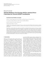
described in [4] with more details. As illustrated in Figure 1,

CogMesh is a self-organized and self-configured hierarchical
network architecture combining the cognitive radio access-
ing technologies with the distributed mesh structure. It
provides an integrated service platform over a wide range
of converged heterogeneous networks, which will enable
opportunistic spectrum access in various licensed and unli-
censed frequency bands. Basically, the CogMesh networking
configuration is restricted by the activity of primary users,
depending on the locally perceived spectrum availability
and the spatial-temporal variations of the primary users’
behavior. This fundamental feature inherently leads to the
natural partitioning of the network architecture. The wireless
network will be partitioned into clusters within which the
involved secondary users agree on one or more common
control channels for networking configuration based on the
2 EURASIP Journal on Advances in Signal Processing
Unlicensed band
Operator B
(CR user)
Operator A
(CR user)
Intra-network spectrum sharing
Operator A
(primary user)
Operator A
(primary user)
Primary user
Spectrum band
CR network
with infrastructure

CR Ad-Hoc network
without infrastructure
Cognitive mesh
Licensed band I
Licensed band II
Inter-network spectrum sharing
CR user
Coexistence with active CR
Figure 1: Cognitive wireless mesh neteworking (CogMesh) scenarios.
locally varying spectrum availability. The clusters themselves
can be reconfigured subject to the presence of the primary
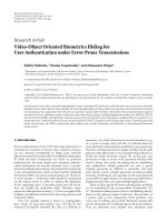
users. Accordingly, the CogMesh network is built by intercon-
necting a number of clusters through various gateway nodes,
as shown in Figure 2. The gateway nodes will transfer data
which includes control channel messages between any two
possible neighboring clusters.
There are two typical cases for intercluster connection:
the two neighbor clusters are overlapping or nonoverlapping.
In the first case, the gateway node is one-hop neighbor of the
two corresponding clusterheads. As depicted in Figure 2,A
and B are clusterheads of cluster A and cluster B, respectively.
C is selected as the gateway node, interconnecting the two
clusters. When the clusterhead A has information (e.g.,
control channel message) sent to the clusterhead B, it firstly
sends the information to node C. Then node C relays it to
the cluster head B. In the reverse path, the cluster head B
sends the information (e.g. control channel message) to node
C, and node C relays it to the clusterhead A. In the second
case, if the two clusters are nonoverlapping but there are
nodes belonging to the two clusters that can hear each other,

they are chosen as the gateway node to interconnect the two
clusters. Because the coordination of the two gateway nodes
needs one more hop, the information exchange in this case is
a little more complex but still follows the same principle and
procedures.
This paper studies the first case and the relevant results
can be easily extended to the second case. We model such
intercluster connection as a two-way relaying channel model
[9]. In the basic scenario, there are two clusterhead A and
B (i.e., two source stations) exchanging the data, including
the control channel message, through the gateway node C
(i.e., relaying). The direct link between A and B is impossible
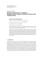
because they are too far away from each other. The traditional
approach, discussed in the previous paragraph, uses a time-
division multirelaying scheme which usually needs four time
slots to complete a round of message exchange (Figure 3(a)).
Recently, network coding, which was first introduced by
Ahlswede et al. [10], has inspired intensive research activities
Cluster A
Cluster B
Cluster D
A
B
D
E
G
C
F
Clusterhead
Gateway node

Ordinary node
Figure 2: Cluster-based network formation in CogMesh.
in the context of wired and wireless networks [11–13].
Network coding can offer network throughput improvement
for two-way communication flows [11, 12].
Moreover, by applying the idea of network coding,
the authors in [11] have proposed a method to reduce
the number of required time-slots from four to three for
internode data exchange. In this method (Figure 3(b)), A
first sends the message X
A
to C during time slot 1, and C
decodes X
A
. During time slot 2, B sends the message X
B
to
C, and C decodes X
B
. In time-slot 3, C broadcasts to A and
B a new message X
C
which consists of bits obtained by bit-
wise exclusive-or (XOR) operations over X
A
and X
B
. Since A
knows X
A

, A can recover its desired message X
B
by decoding
X
C
and then obtaining X
B
as X
A
⊕ X
C
. Similarly, B can
recover X
A
. The principle of network coding has been further
investigated in [12], within which the proposed scheme is
EURASIP Journal on Advances in Signal Processing 3
A
A
A
A
C
C
C
C
B
B
B
B
X

A
X
A
X
B
X
B
(a) Traditional method
A
A
A
C
C
C
B
B
B
X
A
X
B
X
A
XORX
B
X
A
XORX
B
(b) XOR-based network coding

A
A
C
C
B
B
X
A
X
B
X
A
+X
B
X
A
+X
B
(c) ANC-based network coding
Figure 3: Intercluster connection in CogMesh.
named as analogue network coding (ANC). In comparison,
this scheme lets A and B send signals simultaneously in the
first time slot. Then after amplifying, the gateway node C
broadcasts a scaled signal in the second time slot to both A
and B (see Figure 3(c)).
In our paper, we take advantage of the ANC-based net-
work coding scheme for enhancing the data flows across the
neighbor clusters. The obvious advantage of network coding
is that it effectively utilizes the broadcasting nature of wireless
communications to fulfill the data exchange in two time slots.

Generally, the aforementioned network coding approaches
are mainly carried out in interference-free wireline and
wireless networking scenarios. However, due to the PUs’
presence in the context of CogMesh networks, the data flows
including the control channel message exchange between
any two neighboring clusters. This should not violate the
interference and QoS constraints of the locally coexisting
PUs, which gives rise to the unique reason to implement the
network coding scheme and will be specifically dealt with in
the following section of this paper.
A large amount of research work on cognitive radio-
enabled dynamic spectrum access has been mainly concen-
trated on addressing two major technical issues. The first
issue is the detection of spectrum opportunities (“spectrum
holes”) that can be used by the secondary users for trans-
mission. The second one is to develop resource allocation
solutions for efficient usage of the detected “spectrum holes”
for the secondary users while realizing peaceful spectrum
sharing with the primary users. In this paper, another
subject will be addressed as the third challenge. In parallel
with the aforementioned ANC-based approach, we pay
special attention to the interaction of cognitive wireless user
(i.e., gateway node) with its local wireless environment via
a learning processes. We focus on developing intelligent
solutions that can be employed by the gateway node to
improve its relaying performance in the CogMesh framework.
In particular, we aim at exploring how to efficiently predict
the future value function impact of these solutions and then
determine its transmission power level and the associated
relaying strategy over time, based on information about

the current spectrum opportunities, the transmit power
and channel characteristics, and the interaction with the
clustering environment.
Accordingly, unlike the previous work on spectrum
sensing and resource management, our main concern is
how users can predict, adapt to and learn from their
wireless communication environment and optimize the
associated transmission strategies given networking “dynam-
ics” experienced during the multiple-round interactions.
Corresponding to the colocated multiple clusters in the
CogMesh framework, we apply advanced learning techniques
to the gateway node to improve its relaying performance
for effectively increasing the data flows including the control
channel message exchange under various dynamic wireless
environmental constraints, resulting from variations in the
behavior of the wireless sources, such as the stochastic
behavior of the primary users.
Experiencing repeated interaction, the gateway node can
obtain partial historic information of the outcome of the
data flows, from which the estimation of the impact on the
expected future rewards can be performed using different
types of interactive learning. In this paper, we focus on
reinforcement learning because this allows the gateway node
to improve its strategy based only on the knowledge of
its own past received payoffs. Our proposed best response
learning policies are inspired from the Dynamic Program-
ming (DP) and ε-greedy learning for the single agent
interacting with environment. Unlike the aforementioned
two learning policies, the proposed best response learning
explicitly considers the interaction and coupling between the

environment and the gateway node. By applying the best
response learning policies, the gateway node can strategically
predict the impact of current actions on future performance
and then optimally make its decision.
Our work in this paper mainly includes two parts. The
first part gives detailed theoretical analysis about Traditional
Intercluster Connection (TIC) and Network Coding-based
Intercluster Connection (NCIC) in CogMesh. In the second
part of our work, we present reinforcement learning-
based policies for the gateway node selecting appropriate
4 EURASIP Journal on Advances in Signal Processing
Cluster A Cluster B
AB
h
A
h
B
g
C
PT
PR
PT: primary transmitter PR: primary receiver
Figure 4: Two-way relay channel of cognitive users coexisting with
PU.
transmission power level. An intelligent gateway node learns
from interactions with the environment on how to behave
in order to achieve the goal of optimal relaying throughput
in the long run. Accordingly, our contribution is mainly in
three aspects. First, we investigate the intercluster connection
within the framework of CogMesh. Secondly, network coding

is applied to enhance the connection between the neigh-
boring clusters. Thirdly, by further applying reinforcement
learning to select transmission power level at the gateway
node, we get optimal relaying throughput in an interference-
restricted environment. This paper is organized as follows.
Section 2 discusses the traditional and network coding-based
intercluster connection. In Section 3, how to get policies of
selecting transmission power level based on reinforcement
learning are presented. Simulations and results are provided
in Section 4. The conclusion is given in Section 5.
2. Intercluster Connection in CogMesh
As shown in Figure 4, we consider a typical scenario which
has one specific PU link and two neighboring clusters. By
applying opportunistic spectrum access techniques, the PU
and SUs may share the same frequency band W. There are
two intercluster communication flows, A
→ B and B → A,
respectively. The gateway node C performs Amplifying-and-
Forwarding (AF) operation in CogMesh inordertorelay
the data flows across the two neighboring clusters. All SU
nodes are half-duplex within each cluster. X
U
[k] is the signal
transmitted from the secondary user U
∈{A, B, C} in time
slot k. If only one node U
∈{A, B, C} is transmitting, the
received signal at node V
∈{A, B, C}/U in time slot k is
Y

V
[
k
]
= h
UV
X
U
[
k
]
+ g
V
X
P
[
k
]
+ Z
V
[
k
]
,(1)
where g
V
is the channel coefficient between the primary
transmitter (PT) and the secondary receivers V. Z
V
[k] is the

additive white Gaussian noise (AWGN) with zero mean and
variance N
0
. The transmitted signal X
U
[k] has zero mean and
a variance P
U
,andX
P
[k] denotes the transmitted signal from
the PT with zero mean and variance P
p
.h
UV
is the channel
coefficient between U and V, and for analytical simplicity,
h
UV
is assumed to be flat and symmetric in the local cluster
area, which implies
h
AC
= h
CA
= h
A
, h
BC
= h

CB
= h
B
,(2)
If A and B transmit simultaneously, C receives
Y
C
[
k
]
= h
A
X
A
[
k
]
+ h
B
X
B
[
k
]
+ g
C
X
p
[
k

]
+ Z
C
[
k
]
. (3)
Furthermore, the channel coefficientisdenotedby f
U
here, between the secondary user U and the primary receiver
(PR). g is the channel coefficient between PT and PR.In
order to find the routing-rate, we assume that the time-
invariant channels and their coefficients are perfectly known
by all SUs.
In this paper, we are particularly interested in how to
improve the relaying performance of the gateway node and
to increase the routing-rate during the data flow exchange by
exploring the network coding scheme.
Definition 1. During L time slot (ts), A receives b
A
bits
reliably from B and B receives b
B
bits reliably from A, then
the routing-rate is given by
R
=
(
b
A

+ b
B
)
L
[
bits/ts
]
. (4)
In order to ensure the feasibility of data relaying, the
collocated clusters have to follow the following constraints.
(1) Mean-squared error (MSE) constraint. The inter-
ference caused by SUs to PU should not exceed a
certain threshold. The MSE derived by memory-
less estimation of the primary signal at the primary
receiver should be less than or equal to a predefined
value T, which also represents the acceptable QoS
level required by the primary user as indicated in
reference [8].
(2) Maximum transmit power constraint. The transmit
power of an SU should not exceed P. In this paper,
for the sake of simplicity, we assume the following.
(a) The maximum transmit power is same for all SUs,
that is, P
U
≤ P. It is easy to extend the discussion to the case
where P is user dependent.
(b) The clusterheads A and B can transmit with the
maximum transmit power P without violating constraint
(1). Since in this paper we place our emphasis on the gateway
node’s performance, this assumption is especially suitable for

the targeted scenario that PUs appear in the overlap area
of two clusters. PUs are nearer to the gateway node than
the clusterheads such that the transmission power of the
gateway node is constrained by (1) and (a) in (2) while the
two clusterheads can transmit with the maximally permitted
power and still maintain constraint (1) at the same time.
Our future work will discuss other scenarios where the
transmission power of the clusterheads and the gateway node
needs to fully satisfy both (1) and (2).
From now on, we compare the Network Coding-based
Intercluster Connection with the Traditional Intercluster
Connection. The theoretical analysis of the achievable
routing-rates is given in details as follows.
2.1. Traditional Intercluster Connection. As mentioned
above, the clusterhead A transmits in time slot k to the
EURASIP Journal on Advances in Signal Processing 5
gateway node C at first. Then C relays the received signal by
an amplifying factor β
1
under the constraints (1) and (2).
In this case, the optimal amplifying factor for increasing the
relaying throughput can be obtained as
max
P
C
β
1
:=

P

C
h
2
A
P + g
2
C
P
P
+ N
0
s.t.C1:
P
P

f
2
C
P
C
+ N
0

g
2
P
P
+ f
2
C

P
C
+ N
0
≤ T,
C2:P
C
≤ P,
(5)
that is
β
1
= min
⎛
⎝




T

g
2
P
P
+ N
0

−P
P

N
0

h
2
A
P + g
2
C
P
P
+ N
0

(
P
P
−T
)
f
2
C
,

P
h
2
A
P + g
2

C
P
P
+ N
0

,
(6)
where the detailed derivation of (5) is given in the appendix.
Clusterhead B receives a scaled signal in next time slot k +1:
Y
B
[
k +1
]
= h
B
β
1

h
A
X
A
[
k
]
+ g
C
X

P
[
k
]
+ Z
C
[
k
]

+ g
B
X
P
[
k +1
]
+ Z
B
[
k +1
]
.
(7)
Therefore B can receive
b
1,B
= W log
2


1+
h
2
B
h
2
A
Pβ
2
1
h
2
B

g
2
C
P
P
+ N
0

β
2
1
+ g
2
B
P
P

+ N
0

. (8)
Similarly, clusterhead A receives
b
1,A
= W log
2

1+
h
2
A
h
2
B
Pβ
2
2
h
2
A

g
2
C
P
P
+ N

0

β
2
2
+ g
2
A
P
P
+ N
0

,(9)
where
β
2
= min
⎛
⎝




T

g
2
P
P

+ N
0

−
P
P
N
0

h
2
B
P + g
2
C
P
P
+ N
0

(
P
P
−T
)
f
2
C
,


P
h
2
B
P + g
2
C
P
P
+ N
0

.
(10)
Since the total duration is 4 time slots, then the routing-
rate for the Traditional Intercluster Connection is
R
1
=

b
1,A
+ b
1,B

4
. (11)
2.2. Network Coding-Based Intercluster Connection. The clus-
terheads A and B simultaneously transmit in time slot k. C
receives Y

C
[k] and the variance of it is denoted by
σ
2
C
=

h
2
A
+ h
2
B

P + g
2
C
P
P
+ N
0
. (12)
Then following the same optimization approach as
above, the gateway node C can relay Y
C
[k]byanoptimal
amplifying factor α:
α
=


P
C
σ
2
C
(13)
in complying with the constraints (1) and (2), that is,
α
= min
⎛
⎝




T

g
2
P
P
+ N
0

−P
P
N
0
σ
2

C
(
P
P
−T
)
f
2
C
,

P
σ
2
C
⎞
⎠
, (14)
and broadcast it to the clusterheads A and B at the same time.
A receives in the next time slot k +1
Y
A
[
k +1
]
= h
A
αY
C
[

k
]
+ g
A
X
P
[
k +1
]
+ Z
A
[
k +1
]
. (15)
Since A knows its own transmitted signal, it can subtract the
back-propagating-self-interference h
2
A
αX
A
[k] and obtain

Y
A
[
k +1
]
= αh
A

h
B
X
B
[
k
]
+ αh
A
g
C
X
P
[
k
]
+ αh
A
Z
C
[
k
]
+ g
A
X
P
[
k +1
]

+ Z
A
[
k +1
]
,
(16)
which implies that A can receive
b
2,A
= W log
2

1+
h
2
A
h
2
B
Pα
2
h
2
A

g
2
C
P

P
+ N
0

α
2
+ g
2
A
P
P
+ N
0

(17)
Similarly, B receives
b
2,B
= W log
2

1+
h
2
B
h
2
A
Pα
2

h
2
B

g
2
C
P
P
+ N
0

α
2
+ g
2
B
P
P
+ N
0

. (18)
The total duration is 2 time slots in this scheme, so the
achieved routing-rate is
R
2
=

b

2,A
+ b
2,B

2
. (19)
3. Intercluster Relaying Based on
Reinforcement Learning
Reinforcement learning has been successfully used in cogni-
tive radio network for channel assignment and is shown to be
computationally simple and efficient. The signal amplifica-
tion at the gateway node in a dynamic CogMesh environment
can be viewed as a reinforcement learning problem [14]. In
this section, we briefly explain the reinforcement learning
agent in the Network Coding based Intercluster Connection,
and then we present an intelligent approach based on
reinforcement learning to solve the signal amplification
problem.
3.1. Preliminaries of Reinforcement Learning and Problem
Formulation. Hereinafter, we briefly introduce the concept
of reinforcement learning. Inspired by psychological theory,
reinforcement learning is a subarea of machine learning
concerned with how an agent takes actions in an environment
in order to maximize a numerical reward [14]. The dynamic
environment evaluates every action selected by the agent and
a reward is sent back to the agent accordingly. The next
action is chosen by the result of learning. The agent is not
told which actions to take, but instead must discover which
actions yield the most reward by trying them. Reinforcement
6 EURASIP Journal on Advances in Signal Processing

learning algorithms are designed to find a policy that maps
states of the environment to the best act ions of an agent.
The environment is typically formulated as a finite-state
Markov decision process (MDP). Formally, a particular
reinforcement learning model consists of [15]
(A) a set of environment states STATE,
(B) a set of actions ACTION,
(C) a set of scalar rewards in
R.
Regarding the intercluster connection, a reinforcement
learning agent (gateway node) learns from its interaction
with the environment on how to behave in order to achieve
the goal of maximum relaying throughput. We consider the
PU’s transmit power as the environment state, the selection
of transmission power level for data relaying at the gateway
node as the agent’s action, and the achieved routing-rate as
the reward gained by the gateway node.
The agent and environment interact in a sequence of
discrete message exchange rounds, t
= 0, 1, 2, At each
round t, the agent senses the environment state, s
t
∈ STATE,
where STATE is the set of PU’s transmit powers; the agent
selects an action a
t
∈ ACTION(s
t
), where ACTION(s
t

)is
the set of actions available in state s
t
. Corresponding to the
CogMesh environment, we specify M appropriate transmit
power levels: P
1
<P
2
···<P
M
,hereP
M
≤ P
P
. s
t
= i denotes
that the PU’s transmit power is P
i
,atroundt, then STATE
= {1, 2, , M}. And we specify N transmission power levels:
P
C1
<P
C2
< ···<P
CN
,hereP
CN

≤ P. a
t
= j denotes that
the transmission power level of the gateway node is P
cj
at
round t, then ACTION
={1, 2, ,N}. At the next round,
in part as a consequence of its action, the agent achieve
b
t+1
=
⎧
⎪
⎪
⎪
⎪
⎪
⎪
⎪
⎪
⎪
⎪
⎪
⎪
⎪
⎪
⎪
⎪
⎪

⎨
⎪
⎪
⎪
⎪
⎪
⎪
⎪
⎪
⎪
⎪
⎪
⎪
⎪
⎪
⎪
⎪
⎪
⎩
W log
2

1+
h
2
A
h
2
B
PP

Ca
t
h
2
A

g
2
C
P
s
t+1
+ N
0

P
Ca
t
+ A

+W log
2

1+
h
2
A
h
2
B

PP
Ca
t
h
2
B

g
2
C
P
s
t+1
+ N
0

P
Ca
t
+ B

if
P
s
t+1

f
2
C
P

Ca
t
+ N
0

g
2
P
s
t+1
+ f
2
C
P
Ca
t
+ N
0
≤ T,
0, else,
(20)
where A denotes that ((h
2
A
+h
2
B
)P + g
2
C

P
s
t+1
+N
0
)(g
2
A
P
s
t+1
+N
0
)
and B denotes that ((h
2
A
+ h
2
B
)P + g
2
C
P
s
t+1
+ N
0
)(g
2

B
P
s
t+1
+ N
0
),
finds itself in a new environment state, s
t+1
.Ateachround
t, the agent’s policy π
t
(s, a) is the probability that a
t
= a if
s
t
= s.
Formally, the value of a state s under a policy π is defined
as
V
π
(
s
)
= E
π
⎧
⎨
⎩

∞

k=0
γ
k
b
t+k+1
| s
t
= s
⎫
⎬
⎭
, (21)
where E
π
{} denotes the expected value given that the agent
follows policy π,andγ is a parameter called the discount rate,
0
≤ γ ≤ 1. Similarly, we define the value of taking action a
in state s under a policy π,denotedQ
π
(s, a) as the expected
return starting from s, taking the action a, and thereafter
following policy π:
Q
π
(
s, a
)

= E
π
⎧
⎨
⎩
∞

k=0
γ
k
b
t+k+1
| s
t
= s, a
t
= a
⎫
⎬
⎭
. (22)
For any policy π and any state s, the following condition
holds between the value of s and the value of its possible
successor state:
V
π
(
s
)
=


a
π
(
s, a
)

s

Pr
ss


B
s

+ γV
π
(
s

)

, (23)
where Pr
ss

= Pr{s
t+1
= s


| s
t
= s} is the transition
probability and B
s

= E{b
t+1
| s
t
= s, a
t
= a, s
t+1
= s

} is
the expected value of next received bits.
Solving the task of selecting an appropriate transmission
power level means, roughly, finding a policy that achieves
maximum relaying throughput over the long run. A policy
π

is defined to be better than or equal to a policy π if its
expected return is greater than or equal to that of π for all
states. In other words, π

≥ π if and only if V
π


(s) ≥ V
π
(s)
for all s
∈ STATE. There is always at least one policy that is
better than or equal to all other policies, which is an optimal
policy. Although there may be more than one, we denote all
the optimal policies by π
∗
. They share the same state-value
function, called the optimal state-value function, denoted by
V
∗
,anddefinedas
V
∗
(
s
)
= max
π
V
π
(
s
)
, (24)
for all s
∈ STATE. Optimal policies also share the same

optimal action-value function, denoted by Q
∗
,anddefined
as
Q
∗
(
s, a
)
= max
π
Q
π
(
s, a
)
, (25)
for all s
∈ STATE and a ∈ ACTION(s). For the state-action
pair (s, a), this function gives the expected return for taking
action a in state s and thereafter following an optimal policy.
3.2. Relaying Signal Amplification Based on
Reinforcement Learning
3.2.1. Dynamic Programming (DP). The reason to compute
the value function for a policy is to help find better policies.
Suppose that we have determined the value function V
π
for
an arbitrary deterministic policy π. For some state s we would
like to know whether or not it is better to choose an action

a
/
=π(s). The criterion is whether this is greater than or less
than V
π
(s). If it is greater, that is, if it is better to select action
a once in state s and thereafter follow π than it always follows
π, then we would expect that it is better to select a once in s,
and that the new policy π

would be a better one.
Since policy π has been improved to yield a better
policy π

, we can then obtain V
π

and improve it again to
produce a better policy, π

. We can th us obt ai n a se quenc e of
monotonically improving policies and value functions [14]:
π
0
E
→ V
π
0
I
→ π

1
E
→ V
π
1
I
→ π
2
E
→ ···
I
→ π
∗
E
→ V
π
∗
,
(26)
EURASIP Journal on Advances in Signal Processing 7
Initialization
t
= 0,V(s) ∈ R, π(s) ∈ ACTION(s)
for all s
∈ STATE
Repeat
Δ
← 0
For each s
∈ STATE

v
← V(s)
For each a
∈ ACTION
Q(s, a)
←

s

Pr
ss
[b
t+1
+ γV(s

)]
π(s)
← arg max
a

s

Pr
ss

[b
t+1
+ γV(s

)]

V(s)
← max
a

s

Pr
ss

[b
t+1
+ γV(s

)]
Δ
← max(Δ, |v − V(s)|)
t
= t +1
Until Δ <θ(a small positive number)
Algorithm 1: Selection of transmission power level based on DP.
where
E
→ denotes a policy evaluation and
I
→ denotes a policy
improvement. This process must converge to an optimal
policy and optimal value function in a finite number of
iterations, because a finite MDP has only a finite number
of policies. This way of finding an optimal policy is called
dynamic programming. A complete algorithm is given; see

Algorithm 1.
3.2.2. ε-Greedy Policy. The ε-greedy policy chooses an action
that has maximal estimated action value most of the
time. However, they will randomly select an action with
probability ε. That is, all nongreedy actions are given the
minimal probability of selection, ε/
|ACTION(s)|, and the
remaining probability, 1
− ε + ε/|ACTION(s)|,isgivento
the greedy action [14]. Let π

be the intelligent policy, then
Q
π
(
s, π

(
s
))
=

a
π

(
s, a
)
Q
π

(
s, a
)
=
ε
|ACTION
(
s
)
|

a
Q
π
(
s, a
)
+
(
1
−ε
)
max
a
Q
π
(
s, a
)
.

(27)
The algorithm is given, see Algorithm 2.
4. Numerical Results
In this section, we present simulation-based experiments
for testing the intercluster connection in Figure 4. First, we
compare the performances of TIC (Traditional Intercluster
Connection) and NCIC (Network Coding based Intercluster
Connection). Secondly, we quantify the performance of
our proposed learning algorithms. We assume that the
channel coefficients are perfectly known to all nodes in the
simulation. The channel coefficients are given by
g
ij
=

d
−n
ij
, (28)
where d
ij
is the physical distance between nodes i and j,and
n is the path loss exponent. In the simulation, the path loss
exponent is assumed to be 4. Rewriting C1in(5)as
T
≥

1
P
P

+
g
2
f
2
C
P
C
+ N
0

−1
, (29)
we derive
T
≥ T
0
:=

1
P
P
+
g
2
N
0

−1
. (30)

Since even without any channel output, the MSE in esti-
mating the primary transmitted signal is at most P
P
, that
is, T<P
P
.IfT ≥ P
P
, the SU transmission is no longer
constrained by the PU. Therefore, in simulation, the value
assigned to T must satisfy
T
0
≤ T<P
P
. (31)
4.1. Performance Comparison between TIC and NCIC. In this
subsection, we study the performance of TIC and NCIC.
We assume that the frequency bandwidth W
= 1MHz, the
transmission power of PU P
P
= 30 dBm, the variance of
AWG N N
0
= 1 dBm, and Binary Frequency Shift Keying
(BFSK) and Binary Phase Shift Keying (BPSK) are chosen
as the modulation schemes. We use following metrics to
compare NCIC with TIC:
(i) Bit Error Rate (BER): the percentage of erroneous bits

in relayed packets.
(ii) Routing-Rate: this is the total relayed bits during each
time slot.
Figure 5 depicts the BERs of TIC and NCIC with different
modulation schemes (BPSK and BFSK) versus the transmit
power of the gateway node. It can be observed that the BER
performance of NCIC is worse than that of TIC. Figure 6
shows the routing-rates of TIC and NCIC whereas NCIC
outperforms TIC. Interestingly, the curves in two figures
approach constant values no matter how the transmit power
at the gateway node increases; for example, the error floors
takes place in Figure 6. This is because the interference
caused by SUs to PUs increases as the gateway node raises
its transmission power such that the MSE constraint by PUs
dominates finally, which restricts the available transmission
power level of the gateway node.
As illustrated in Figures 5 and 6, in regard to improving
the data relaying throughput across the neighboring clusters,
NCIC performs substantially well over TIC. Therefore, NCIC
is more suitable than TIC, since the relaying throughput is
taken more seriously during the data flowing procedure.
On the other hand, concerning the initial cluster setting-
up stage for CogMesh networking formation, especially if we
want to guarantee reliability for the critical control channel
message exchange, TIC is preferable because it provides
robust message exchange in the interference-deteriorated
channel even though it losses the routing-rate to some extent.
4.2. Impact of Dynamic Environment on Learning Policies. We
present numerical results to compare the performances of the
8 EURASIP Journal on Advances in Signal Processing

Initialize, for all s ∈ STATE, a ∈ ACTION(s):
N
← 0, γ ← an arbitrary between 0 and 1
Q(s, a)
← arbitrary
b(s, a)
← empty list
π
←arbitrary
Repeat forever:
(a) N
← N +1
(b) Generate an episode using π
(c) For each pair s, a appearing in the episode:
b
N
=
⎧
⎪
⎪
⎪
⎪
⎪
⎪
⎪
⎪
⎪
⎪
⎪
⎪

⎪
⎪
⎪
⎪
⎪
⎨
⎪
⎪
⎪
⎪
⎪
⎪
⎪
⎪
⎪
⎪
⎪
⎪
⎪
⎪
⎪
⎪
⎪
⎩
W log
2

1+
h
2

A
h
2
B
PP
Ca
h
2
A
(g
2
C
P
s
+ N
0
)P
Ca
+((h
2
A
+ h
2
B
)P + g
2
C
P
s
+ N

0
)(g
2
A
P
s
+ N
0
)

+W log
2

1+
h
2
A
h
2
B
PP
Ca
t
h
2
B
(g
2
C
P

s
+ N
0
)P
Ca
+((h
2
A
+ h
2
B
)P + g
2
C
P
s
+ N
0
)(g
2
B
P
s
+ N
0
)

if
P
s

( f
2
C
P
Ca
+ N
0
)
g
2
P
s
+ f
2
C
P
Ca
+ N
0
≤ T
0, else
for the first occurrence of s, a
Q(s, a)
← Q(s, a)+γ
N−1
b
N
(d) For each s in the episode
a
∗

← arg max
a
Q(s, a)
For all a
∈ ACTION(s):
π(s, a)
←
⎧
⎪
⎪
⎪
⎨
⎪
⎪
⎪
⎩
1 −ε +
ε
|ACTION(s)|
,ifa = a
∗
ε
|ACTION(s)|
if a
/
=a
∗
Algorithm 2: Selection of transmission power level based on ε-greedy policy.
10
−4

10
−3
10
−2
10
−1
10
0
BER
0 5 10 15 20 25 30
Pc (dBm)
TIC: BFSK
NCIC: BFSK
TIC: BPSK
NCIC: BPSK
Figure 5: BER versus P
c
.
intelligent relaying signal amplification based on DP and ε-
greedy policies. During the whole simulation processes, we
specify 3 transmission power levels of PU: 20 dBm, 25 dBm,
30 dBm, with the corresponding state set STATE
={1, 2, 3},
0
0.5
1
1.5
2
2.5
3

3.5
4
4.5
Routing rate (Mbits/ts)
0 5 10 15 20 25 30
Pc (dBm)
TIC: T
= 0.02
NCIC: T
= 0.02
TIC: T
= 0.01
NCIC: T
= 0.01
Figure 6: System throughput versus P
c
.
and specify 20 transmission power of the gateway node:
11 dBm, 12 dB, 13 dBm, , 30 dBm, with the corresponding
action set ACTION
={1, 2, ,20}. The other parameters
are set as follows: QoS requirement T
= 0.02, discount rate
γ
= 0.9, and ε = 0.3.
EURASIP Journal on Advances in Signal Processing 9
0
5
10
15

20
25
30
35
40
45
State value function
10
0
10
1
10
2
10
3
Iteration
State:1
State:2
State:3
State value function for optimal policy
Figure 7: State value function versus t for DP-based policy.
0
0.1
0.2
0.3
0.4
0.5
0.6
0.7
0.8

0.9
1
Probability
0 100 200 300 400 500 600
Iteration
State:1, action: 13
State:2, action: 13
State:3, action: 13
ε-greedy MC method
Figure 8: Probability of optimal policy at different states for ε-
greedy-based policy.
In Figure 7, we characterize the convergence behavior of
the state value functions for DP-based policy. It can be seen
that the numbers of iterations are no more than 100. Figure 8
shows convergence behavior of the probabilities of optimal
policies in different states for ε-greedy policy.
The BER dynamics of the DP-based policy and ε-greedy
policy are shown in Figure 9 and the routing-rate dynamics
are shown in Figure 10. We can see that the ε-greedy policy
cannot achieve better performance than DP-based policy
since it always gives the probability ε/
|ACTION(s)| to select
the available actions randomly.
10
−2
10
−1
Expected BER
0 100 200 300 400 500 600
Iteration

DP-based policy
ε-greedy policy
Figure 9: BER comparison between DP-based policy and ε-greedy
policy.
2
2.5
3
3.5
4
4.5
5
Expected routing-rate (Mbits/ts)
0 100 200 300 400 500 600
Iteration
DP-based policy
ε-greedy policy
Figure 10: Relay rate comparison between MDP-based policy and
ε-greedy MC-based policy.
5. Conclusion
This paper investigates the intercluster connection issue
within the framework of CogMesh networks. Corresponding
to the distributed secondary users, all transmissions should
satisfy the QoS and interference constraints imposed by
the primary users. The Traditional Intercluster Connection
scheme cannot achieve scheduling and routing multiple
data flows at the same time because they may interfere
with each other. Therefore, the Network Coding-based
Intercluster Connection scheme, which allows multiple data
flows to be transmitted simultaneously across the neigh-
boring clusters under the QoS and interference constraint

10 EURASIP Journal on Advances in Signal Processing
by PUs, is proposed. Our simulation experiments show
that the Network Coding-based Intercluster Connection
has a significant advantage over the Traditional Intercluster
Connection in the data relaying procedure. However, in
the initial cluster formation stage especially concerning the
critical control channel message exchange, the Traditional
Intercluster Connection is preferable because it provides
robust data relaying in the interference-restricted channel
even though it losses the routing-rate to some extent.
Moreover, based on reinforcement learning, we address
the problem of how to choose the optimal transmission
power level at the gateway node for enhancing the data
relaying throughput. Two intelligent policies, namely, the
DP-based policy and the ε-greedy policy, are investigated
which take the clustering environment status into account.
The novel feature of the intelligent policies is that without
perfect knowledge of the primary user’s transmit power and
QoS requirement the gateway node can optimize the relaying
throughput by interacting with the environment in the long
run. Due to the fact that it gives a certain opportunity to
select the available actions in the environment state, the
ε-greedy policy converges to, but can never achieve, the
performance of DP-based policy.
Appendix
Derivation of C1 in (5)
In this section, we introduce a simplified channel model; as
shown in Figure 7, the PU receives signal
Y
P

(
n
)
= gX
P
(
n
)
+ f
C
X
C
(
n
)
+ Z
P
(
n
)
,(A.1)
where n denotes the sampled discrete time, and Z
P
(n) is the
AWGN with zero mean and variance N
0
.
Let X
P
(n) be an unknown random variable, and let Y

P
(n)
be a known random variable. What is the best guess of X
P
(n),
given Y
P
(n), in the MMSE sense? That is, we want to find
afunction

X
P
(n) = b(Y
P
(1) ···Y
P
(n)) such that we can
minimize
MSE
= E




X
P
(
n
)
−


X
P
(
n
)




. (A.2)
The expectation is taken over both X
P
(n)andY
P
(n).
In this paper, we restrict the functional form of b(
·)tobe
homogeneous linear; that is,

X
P
(n) =

m
i
=1
b
i
Y

P
(n − i +1),
and we want to minimize
MSE
= E
⎧
⎪
⎨
⎪
⎩






X
P
(
n
)
−
⎛
⎝
m

i=1
b
i
Y

P
(n − i +1)
⎞
⎠






2
⎫
⎪
⎬
⎪
⎭
. (A.3)
Equation (A.3) can be expressed in a compact form
MSE
= E




X
P
(
n
)
−b

T
Y
P



2

,(A.4)
where
b
=
[
b
1
b
m
]
T
,
Y
P
=
[
Y
P
(
n
)
Y

P
(
n
−m +1
)
]
T
.
(A.5)
The solution for b can be found out from ∂MSE/∂b
= 0,
that is,
∂MSE
∂b
= E

∂
∂b



X
P
(
n
)
−b
T
Y
P




2

=−
2R
XY
+2b
T
R
Y
= 0,
(A.6)
where R
XY
= E{X
P
(n)Y
∗
P
} and R
Y
= E{|Y
P
|
2
}.Thusweget
b
T

= R
XY
R
−1
Y
. (A.7)
Combining (A.7)and(A.4), the minimum MSE is given
MMSE
= P
P
−R
XY
R
−1
Y
R
YX
. (A.8)
Following, we present a detailed analysis into the deriva-
tions of cross-correlation matrix R
XY
and autocorrelation
matrix R
Y
. Here, we assume that the transmitted signals are
uncorrelated, then
R
XY
= E


X
P
(
n
)
·

Y
∗
P
(
n
)
Y
∗
P
(
n
−m +1
)

=
E

g ·X
P
(
n
)
·


X
∗
P
(
n
)
X
∗
P
(
n
−m +1
)

=
gP
P
[
10 0
]
.
(A.9)
In the same way, we can derive
R
Y
= E
⎧
⎪
⎪

⎪
⎪
⎨
⎪
⎪
⎪
⎪
⎩
⎡
⎢
⎢
⎢
⎢
⎣
Y
P
(
n
)
.
.
.
Y
P
(
n
−m +1
)
⎤
⎥

⎥
⎥
⎥
⎦

Y
∗
p
(
n
)
Y
∗
p
(
n
−m +1
)

⎫
⎪
⎪
⎪
⎪
⎬
⎪
⎪
⎪
⎪
⎭

=

g
2
P
P
+ f
2
C
P
C
+ N
0

⎡
⎢
⎢
⎢
⎢
⎢
⎢
⎢
⎢
⎣
10··· 0
01
.
.
.
.

.
.
.
.
.
.
.
.
.
.
.
0
0
··· 01
⎤
⎥
⎥
⎥
⎥
⎥
⎥
⎥
⎥
⎦
.
(A.10)
The inverse of R
Y
is
R

−1
Y
=
1
g
2
P
P
+ f
2
C
P
C
+ N
0
⎡
⎢
⎢
⎢
⎢
⎢
⎢
⎢
⎢
⎣
10··· 0
01
.
.
.

.
.
.
.
.
.
.
.
.
.
.
.
0
0
··· 01
⎤
⎥
⎥
⎥
⎥
⎥
⎥
⎥
⎥
⎦
. (A.11)
Hence, by combining (A.8), (A.9), and (A.11), the minimum
MSE can be expressed as
MMSE
= P

P
−
g
2
P
2
P
g
2
P
P
+ f
2
C
P
C
+ N
0
=
P
P

f
2
C
P
C
+ N
0


g
2
P
P
+ f
2
C
P
C
+ N
0
.
(A.12)
If the PU imposes a QoS requirement on the MMSE, in
other words, the PU’s MMSE should not exceed a predefined
T. Finally, the constraint C1 in(5)
P
P

f
2
C
P
C
+ N
0

g
2
P

P
+ f
2
C
P
C
+ N
0
≤ T (A.13)
is obtained.
EURASIP Journal on Advances in Signal Processing 11
References
[1] Federal Communications Commission, “Spectrum Policy
Task Force,” Tech. Rep. ET Docket 02-135, November 2002.
[2] J. Mitola III and G. Q. Maguire Jr., “Cognitive radio: making
software radios more personal,” IEEE Personal Communica-
tions, vol. 6, no. 4, pp. 13–18, 1999.
[3] S. Haykin, “Cognitive radio: brain-empowered wireless com-
munications,” IEEE Journal on Selected Areas in Communica-
tions, vol. 23, no. 2, pp. 201–220, 2005.
[4] T. Chen, H. Zhang, G. M. Maggio, and I. Chlamtac,
“CogMesh: a cluster-based cognitive radio network,” in Pro-
ceedings of the 2nd IEEE International Symposium on New
Frontiers in Dynamic Spectrum Access Networks (DySPAN ’07),
pp. 168–178, April 2007.
[5]Y.ShiandY.T.Hou,“Adistributedoptimizationalgorithm
for multi-hop cognitive radio networks,” in Proceedings of the
27th IEEE Communications Society Conference on Computer
Communications (INFOCOM ’08), pp. 1292–1300, Phoenix,
Ariz, USA, April 2008.

[6] L. Zhang, Y. Xin, and Y C. Liang, “Power allocation for multi-
antenna multiple access channels in cognitive radio networks,”
in Proceedings of the 41st Annual Conference on Information
Sciences and Systems (CISS ’07), pp. 351–356, Baltimore, Md,
USA, March 2007.
[7] F. Wang, M. Krunz, and S. Cui, “Price-based spectrum
management in cognitive radio networks,” IEEE Journal on
Selected Topics in Signal Processing, vol. 2, no. 1, pp. 74–87,
2008.
[8] W. Zhang and U. Mitra, “A spectrum-shaping perspective on
cognitive radio,” in Proceedings of the 3rd IEEE Symposium on
New Frontiers in Dynamic Spectrum Access Networks (DySPAN
’08), pp. 1–12, Chicago, Ill, USA, October 2008.
[9] C. E. Shannon, “Two-way communication channels,” in
Proceedings of the 4th Berkeley Symposium on Mathematical
Statistics and Probability, vol. 1, pp. 611–644, 1961.
[10] R. Ahlswede, N. Cai, S Y. R. Li, and R. W. Yeung, “Network
information flow,” IEEE Transactions on Information Theory,
vol. 46, no. 4, pp. 1204–1216, 2000.
[11] S. Katti, H. Rahul, W. Hu, D. Katabi, M. Medard, and
J. Crowcroft, “XORs in the air: practical wireless network
coding,” in Proceedings of the Conference on Applications,
Technologies, Architectures, and Protocols for Computer Com-
munications (SIGCOMM ’06), Pisa, Italy, September 2006.
[12] S. Katti, I. Mari
´
c, A. Goldsmith, D. Katabi, and M. Medard,
“Joint relaying and network coding in wireless networks,” in
Proceedings of the IEEE International Symposium on Informa-
tion Theory (ISIT ’07), pp. 1101–1105, Nice, France, June 2007.

[13] Y. Wu, P. A. Chou, and S Y. Kung, “Minimum-energy
multicast in mobile ad hoc networks using network coding,”
IEEE Transactions on Communications, vol. 53, no. 11, pp.
1906–1918, 2005.
[14] R. S. Sutton and A. G. Barto, Reinforcement Learning: An
Introduction, MIT Press, Cambridge, Mass, USA, 1998.
[15] L. P. Kaelbling, M. L. Littman, and A. W. Moore, “Rein-
forcement learning: a survey,” Journal of Artificial Intelligence
Research, vol. 4, pp. 237–285, 1996.