Machining of High Strength Steels With Emphasis on Surface Integrity by air force machinability data center_1 pot
Bạn đang xem bản rút gọn của tài liệu. Xem và tải ngay bản đầy đủ của tài liệu tại đây (318.08 KB, 9 trang )
7
Machinability and Surface Integrity
‘It is common sense to take a method and try it.
If it fails, admit it frankly and try another.
But above all, try something. ’
(1882 – 1945)
[32
nd
President: United States of America]
7.1 Machinability
Introduction – an Historical Perspective
Today, greater emphasis is being placed on a compo-
nent’s ‘machinability’ , but this term is an ambiguous
one, having a variety of dierent meanings, depending
upon the production engineer’s requirements. In fact,
the machinability expression does not have an author-
itative denition, despite the fact that it has been used
for decades. In 1938, Ernst in his book on the ‘Physics
of Metal Cutting’ , dened machinability in the follow
-
ing manner:
‘As a complex physical property of a metal involving:
•
True machinability, a function of the tensile strength,
•
Finishability, or ease of obtaining a good nish,
•
Abrasiveness, or the abrasion undergone by the tool
during cutting.’
By 1950, Boulger had summarised these criteria more
succinctly in his statement: ‘From any standpoint, the
material with the best machinability is the one permit-
ting the fastest removal of chips with satisfactory tool
life and surface nish.’ is ‘Boulger denition’ leaves
some unanswered questions concerning chip-form-
ing factors, cutting forces and, has little regard for
either the physical and mechanical properties of the
material, nor potential sub-surface damage caused by
the cutting edge. By 1989, Smith made the point that
in fact machinability, had to address these properties
and the word ‘metal’ should be substituted by the ex-
pression ‘material’ , in a combined general-purpose
denition, as follows: e totality of all the properties
of a work material which aect the cutting process and,
the relative ease of producing satisfactory products by
chip-forming methods.’ Even these denitions still lack
sucient precision to be of much practical use and by
1999, Gorzkowski, et al., in their powder metallurgy
paper concerning ‘secondary machining’
1
, entitled:
1 ‘Secondary machining’ , is a term used to cover any additional
post-machining operations (e.g. drilling, turning and milling,
etc.), that has to be undertaken on powder metallurgy (i.e.
sintered’) compacts, aer compaction and sintering. Nor-
mally, these post-sintering production processes, are only car-
ried out to ensure, say: a good turned registered diameter, a
precision cross-drilled hole, precise and accurate screwthread,
an undercut, or similar* – as this is a last resort, as it adds-
value to the overall component’s cost.
‘Machinability’ , stated that: ‘Machinability is a dicult
property to quantify.’ Why is this so? It is probably is
a combination of many inter-related factors, such as:
chemical composition of the workpiece, its micro-
structure, heat-treatment, purity, together with many
more eects which inuence the overall machining
operation. In Fig. 144, this diagram attempts to high-
light some of the important factors that aect a com-
ponent’s machined state – its ‘machinability’. Although
even here, an important factor such as power con-
sumption is missing, showing that this is by no means
an exhaustive ow-chart of the complex mechanisms
that exist when a material is subjected to machining.
is is probably why it is virtually impossible to state
that one, or another material aer machining, was ei-
ther a ‘good’ , or bad’ one to machine. By utilising some
‘impartial and objective testing program’ , it may be pos-
sible to ‘rank’ prospective or current materials, or pro-
duction tools – in some way, perhaps by way of a ‘De-
sign of Experiments’ (DoE), in combination with ‘Value
Analysis’ (VA) approach to the production problem.
is strategic technique to the problems of ‘machin-
ability comparisons’ of diering factors will shortly be
mentioned in more detail, aer a brief resumé on just
some of the machinability testing techniques favoured
today.
.. Design of Machinability
Tests and Experimental
Testing Programmes
Over the years, a range of machinability testpieces
have been developed – more on this shortly – that are
used to assess specic cutting conditions found when
machining the actual production part. e assessment
of a material’s machinability can be undertaken by two
groups of tests, these are machining and non-machin-
ing testing programmes. e former machinability
group, can be further sub-divided into either ‘ranking’
and ‘absolute’ tests and, it should be mentioned that
the latter non-machining tests fall into the ranking
category. Oen, ‘ranking’ tests are termed ‘short
*Powders when they ll the dies and are compacted, cannot
reproduce component features at 90° to the major pressing di-
rection – hence, the powders cannot readily move sideways –
as such, features, like: screwthreads, transversal features (i.e.
undercuts, etc.), must be machined aerward, hence, the term
‘secondary machining’.
Chapter
Figure 144. The major factors that inuence a machined component’s condition.
Machinability and Surface Integrity
tests’ , conversely ‘absolute’ tests are known as ‘long
tests’. By their very nature, the ‘short tests’ merely in-
dicate the relative machinabilities of two, or more dif-
ferent combinations of tool and workpiece. Whereas,
the ‘long tests’ can produce a more complete depiction
of the anticipated conditions for various combinations
of tool and workpiece, but as their name suggests,
they are more time-consuming and costly to develop
and perform. Some of these test regimes are briey
reviewed below, but more information can be obtained
from the listed references at the end of this chapter.
‘Ranking’ Machining Tests
A series of these ‘ranking’ tests for fast assessment of
actual production conditions has been devised over
the years and some will be mentioned below, but this is
by no means an exhaustive account of all such testing
programmes, they merely indicate the relatively well-
tried-and-tested techniques, such as:
•
‘Rapid facing test’ – this consists of a turning op-
eration, requiring facing-o a workpiece, preferably
having a large diameter, using an HSS tool
2
. e
machinability is assessed by the distance the tool
will travel radially-outward, from the bar’s centre,
prior to its catastrophic tool failure. is ‘end-
point’ as it is known, is compared with a similar
trial, where the distance for tool failure by using a
reference material
3
was previously determined,
NB Although the ‘Rapid facing test’ quickly assesses
one particular test criterion that a machinability
rating can be based upon, it suers from a number
of limitations. Firstly, the material’s diameter may
be smaller than that which one would ideally prefer
to use for the test. Secondly, if the workpiece mate-
rial’s structure is not homogeneous
4
, then this test
only indicates properties over the diameter-range
2 ‘HSS tool material’ is utilised, because under these extreme
machining conditions, it will rapidly promote catastrophic
tool failure as the forces steadily increase together with esca-
lating tool interface temperature, as the tool’s edge is fed radi-
ally-outward during the subsequent facing operation.
3 ‘Reference materials’ , are normally those workpiece materials
that are considered to be ‘easy-to-machine’ , as their name sug-
gests they, at the very least, give a ‘base-line’ , or datum, for
some form of machinability comparison.
4 ‘Homogeneity of material’ , refers to a uniformity of its micro-
structure and having isotropic properties.
used. is latter problem of lack of homogeneity of
the workpiece material, can be somewhat lessened
by boring-out the material at the workpiece’s cen-
tre, prior to commencing the test.
•
‘Constant-pressure test’ – this is quite a popular
testing technique and can be undertaken by a va-
riety of methods of machining assessment. For
example, in turning, machinability is measured by
utilising predetermined geometry in association
with a constant feed force. e technique has been
used to some eect on the machining of free-cut-
ting steels. is test is essentially a measure of the
friction between the chip and tool, which is re-
lated to the specic cutting temperatures generated
whilst machining, together with its eects on the
tool’s wear-rate,
NB Normally a turning centre has a constant feed
force, in order to obtain relevant data. An engine-/
centre-lathe can also be employed to acquire iden-
tical data, but a tool-force dynamometer is used
to measure this feed force, then plotting a graph
of this feed force with its associated frictional ef-
fects, but this requires more eort and takes longer.
Similar constant pressure tests can be employed for
drilling processes.
•
‘Degraded tool test’ – consists of workpiece ma-
chining with a soened (i.e. degraded) cutting tool.
e test’s ‘end-point’ is determined either: when a
specied amount of tool ank/crater wear has been
reached, or at catastrophic tool failure,
NB If machinability testing is carried out on soer
and more easy-to-machine materials – typically on
various alloys of brass, then just a small variation in
soening the tool steel prior to cutting, has a dras-
tic eect on the results obtained, but for harder-to-
machine materials this eect is signicantly less-
ened.
•
‘Accelerated cutting-tool wear test’ – as an alterna-
tive to deliberately soening the tool (i.e. Degrad-
ing tool test), in order to speed-up the machinabil-
ity process the cutting speeds are increased. If the
cutting speeds are signicantly increased, the tool
will not behave according to the predictable tool life
Chapter
equation
5
– due to the articially-elevated cutting
temperature generated.
NB It is not prudent practice to extrapolate tool-
life data beyond that actually obtained during test-
ing in order to obtain quantitative information
about other ranges and conditions, with diering
operations and parameters. As a result, this test is
usually classied as a ‘ranking test’.
‘Ranking’ – Non-Machining Tests
Whenever there seems to be a need to experiment with
material cutting using perhaps one of the techniques
just mentioned, it is important to establish whether
any savings gained will be recouped in the actual pro-
duction operation. If a company is unsure of the likely
cost benets of such testing, then a strong case can be
made not to test the material at all! Fortunately, non-
machining tests exist that can be utilised in these doubt-
ful situations, rather than ‘working blindly’ – with no
relevant cutting data, to base the applied cutting con-
ditions upon. Several of these ‘ranking’ non-machining
tests can be employed, such as:
•
Chemical composition test – a variety of tests have
been developed by which workpiece materials are
‘ranked’ according to their primary constituents. It
is obvious that the results from such tests are only
relevant when materials of similar type, having
identical processing conditions/thermal history
6
,
are to be machined.
5 Taylor’s tool life equation(s), has been utilised for many years,
to determine the ‘end-point’ of a cutting insert’s useful life,
under steady-state cutting conditions. e basis of the general
formula: V
c
T
α
= C, has been modied and expanded to obtain
an equation for the ‘economical cutting-edge life’ for a speci-
ed feed, as follows:
T
e
= (1/α – 1)(C
t
/C
m
+ t
c
)
Where: T
e
= economical tool life, α = slope of the VT-curve (i.e.
measured from a plotted graph), C
t
= cutting-tool cost per
cutting edge (i.e. see ‘Machining costs’ – later in the chapter),
C
m
= machine charge per minute (i.e normally established by
the machine shop management), t
c
= tool-changing time for
the cutting operation – this will vary according to whether the
tooling is of the conventional, or quick- change type.
6 ‘ermal history’ , refers to the heat treatment thermal cycle
that the component in question was processed, describing the
time at temperature, with any modications to the tempera-
ture-induced regime on the heat-treated part.
NB Given the above limitations, these tests have
proved to be quite valid and successful for screen-
ing a workpiece material prior to actual machining.
Typical examples of this test type, rank materials
using a V
60
scale – giving cutting speeds in m min
–1
and the machinability index of 100 (i.e. utilised by
the ‘Volvo test’ – not shown). A close correlation be-
tween the chemical composition test and ‘absolute
tests’ has been obtained with accuracies claimed
to within 8%. For example, the relationship be-
tween chemical composition and cutting speed is:
Cutting speed (V
60
) = 161.5 – 141.4 × %C – 42 – 4 ×
%Si – 39.2 × %Mn – 179.4 × %P + 121.4 × %S.
•
Microstructure tests – are principally concerned
with the type of microstructure present in say, a
steel workpiece, specically: inclusion type, shape
and dispersion. e test method gives a good in-
dication of the likely machinability, but requires
highly-specialised laboratory equipment for such a
metallographical investigation although materials
can only be ranked, as either: good, bad, or indier-
ent.
NB Early work here, primarily investigated low-
to-medium carbon steel microstructures, notably
considering the spacing between pearlite laminae
achieved by heat treatment. e pearlite-to-ferrite
proportions clearly inuenced the materials hard-
ness value (e.g. Brinell). When a cutting speed was
selected (e.g. V
80
), a machinability rating could be
obtained for either life at: a constant speed (min-
utes), or relative speed for a constant tool life
(m min
–1
). It has been observed that when >50%
pearlite was present, combined with a relatively high
bulk hardness
7
, then good machining characteristics
occurred. In recent years, commercially-available
steels have trace elements added to aid machinabil-
ity, the so-called free-machining steels. Typically,
sulphur and manganese additions, create manga-
nese sulphide, with their shape, size and distribu-
tion within the steel’s matrix, playing a major role
in aiding machinability factors.
7 ‘Bulk hardness’ , is a term that is used to state the overall hard-
ness of the test specimen, not its micro-hardness – which only
establishes localised hardness levels.
Machinability and Surface Integrity
•
Physical properties test – requires specialist equip-
ment in order to perform this test. e physical
properties of the workpiece material are utilised in
order to determine its machinability ranking.
NB Researchers, have produced a general machin-
ability equation using a dimensional analysis tech-
nique and, by utilising conventional test methods
to establish and measure its: thermal conductivity,
harness (Brinell), percentage reduction in area,
together with the test sample’s length. is ‘Physi-
cal properties test’ , gives close agreement with the
V
60
cutting speed for a range of ferrous alloys, al-
though when brittle materials are assessed, the lack
of a yield-point
8
and the much smaller reductions
in area – aer tensile testing – may cause potential
ranking problems.
‘Absolute’ Machining Tests
As their name implies, the ‘absolute tests’ are utilised
in order to obtain a comprehensive data-gathering
machining-based activity, on particular types of work-
piece and cutting tool combinations. Many of these
‘absolute testing’ techniques have been devised, with
several of them listed below, including the:
•
Taper-turning test – being undertaken by turning a
tapered workpiece. As a result of turning along the
taper, the cutting speed will proportionally increase
with increasing taper diameter – this also being in
proportion to the cutting time. By originally estab-
lishing the cutting speed, the changing-rate of the
8 ‘Yield-point’ , refers to the strain* at which deformation be-
comes permanent, when the material is subjected to some
form of mechanical-working. e yield-point strain for fer-
rous and many ductile materials is well-dened, illustrating a
‘sharp’ transition from elastic-to-plastic deformation – where
a permanent ‘set’ occurs. However, this is not the case for
many brittle materials, here when say, a tensile test is con-
ducted, an articial ‘proof-stress’ value is used to intersect the
stress/strain curve plotted, to establish its safe-working level
of operation – see the relevant References for more in-depth
details.
*‘Strain’ , is a measure of the change in the size, or shape
of a body – referring to its original size, or shape. For ex-
ample, linear strain is the change per unit length of a linear
dimension – aer some form of mechanical working. For a
tensile test specimen that has been subjected to a tensile test, it
refers to its linear dimensional change from its original gauge
length.
cutting speed in conjunction with the amount of
tool ank wear – for two separate tests – allows the
values of the constants (i.e.‘α’ and ‘C’) in Taylor’s
equation for tool wear – see Footnote 5 – to be de-
rived and, the tool life established for a range of fu-
ture cutting tests. As the D
OC
must be consistently
maintained throughout the test, either a CNC pro-
gram must be written – using one of the standard
‘canned-routines’ available, or a taper-turning at-
tachment is necessary on an engine-/centre-lathe,
NB Some major advantages accrue from this com-
prehensive testing technique, not least of which is
that results are valid for a range of pre-selected cut-
ting speeds and, the test is of relatively short du-
ration, but closely agree with many thorough and
longer test methods. Although, the results obtained
may not be representative of actual cutting condi-
tions, owing to the fact that the cutting tool, ma-
chines at diering diameters throughout the taper
turning test.
•
Variable-rate machining test – achieves similar
results to the previously described ‘Taper-turn-
ing test’. In this case, the increase in cutting speed
is obtained by turning a parallel testpiece axially,
whilst simultaneously increasing the cutting speed
as the tool traverses longitudinally along the work-
piece. Once again, the constants are derived for the
‘Taylor equation’ aer a minimum of two tests have
been completed,
NB e main advantages of this method over the
‘Taper-turning test’ , are that a standard testpiece
can be used and the results probably reect truer
actual turning conditions – in that consistent diam-
eters are being turned, although this argument is
somewhat debased, if the turning of complex free-
from component geometry is demanded for the
production part.
•
Step-turning test – was developed to overcome
some of the problems associated with the two pre-
viously described testing techniques. In the ‘Step-
turning test’ method, a range of discrete diameters
and speeds are utilised to determine the ‘Taylor’s
constants’. is test, shows close agreement with re-
sults obtained from the two previously-mentioned
‘absolute test’ methods,
•
HSS tool wear-rate test – this test assesses machin-
ability by measurement of the tool’s ank wear, pro-
Chapter
duced when machining free-cutting steels, with the
major parameters being the elemental additions to
the metallurgical composition of these steel grades.
NB ese tests are undertaken in a similar manner
to the: ISO 3685:1977 Standard, for a long ‘absolute
test’ , but it was withdrawn in mid-1984.
All of the above ‘absolute testing’ programmes, relate
to turning operations, principally due to the fact that
the tool is engaged in the workpiece test sample for a
reasonably lengthy period of time. is tool/workpiece
engagement, allows for ‘steady-state’ conditions to be
developed, having the additional benet of producing
relatively consistent ‘Taylor constants’. From a more
practical viewpoint, the author has developed some
other testpieces, which have proved somewhat useful
in actual industrial machining applications, where a
more representative machinability situation was de-
manded. Just some of these testpieces, along with a
discussion of their relative merits, will now proceed.
Practical Testpieces – for CNC Applications
e premise behind the development of the testpiece
depicted in Fig. 145, was to attempt to ‘mirror’ the ac-
tual production operations and to a lesser extent, the
physical geometry of a particular component part.
Here, the component geometry was devised to be ma-
chined on either a machining centre, or a turning cen-
tre with the facility of driven tooling and at the very
least, having an indexing workholding spindle/chuck.
With this testpiece, the part is preferably a thick-walled
tube that can be bored out, OD turned, circular inter-
polated (i.e. milled), drilled and tapped – as the drill-
ing size, is also an M6x1 tapping size. is allows the
component’s geometric features to be inspected ‘On-
machine’ – using metrological inspection routines in
association with touch-trigger probes and, ‘O-ma-
chine’ employing a CNC Co-ordinate Measuring Ma-
chine (CMM). ese identical parts were from a series
of exhaustive tests undertaken on both ferrous metals
and aerospace-grade aluminium stock. Of particular
note, was that when a milled circular interpolated fea-
ture – the boss, was assessed on the machining centre,
it gave more accurate readings than its equivalent in-
spection routine on the CMM. is perceived dier-
ence in accuracy and precision, was the result of part
changes caused by both relaxation of the clamping
forces – upon release – and the greater temperature
dierential between these workpieces when inspected
on the CMM. However of note, was the fact that in
general for the inspection of part features, the CMM
showed a four times improvement in repeatability, to
that of the touch-trigger probing undertaken on the
machine tool, as the following Table 9 indicates:
e above type of practical ‘testing regimes’ are gen-
erally termed: ‘Production Performance Tests’ (PPT).
Typically, these PPT’s can be utilised to determine the
maximum production rate – in parts per hour. Al-
though it must be said, that with shis normally con-
sisting of between 6 to 8 hours duration of potential
‘in-cut time’ , this to a certain extent, limit’s the achiev
-
able machined surface nish requirement, particularly
if a ‘Sister tooling strategy’ is not operated. One of the
main problems connected with PPT’s, is that invari-
ably free-cutting metals are usually selected for long-
term testing, meaning that any wear-related data takes
awhile to accrue. Despite this slight reservation, actual
cutting data can be employed, which represents almost
optimum machining conditions, leading the way to
Table 9. A comparison of the machined component tes-
tpiece accuracies by either: ‘On-’ , or ‘O-machine’ inspection
procedures
PARAMETERS: MACHINES*:
- equipped with Renishaw touch-
trigger probes:
Machining Centre
(Vertical)
CMM (LK CNC
Micro4)
Scope Full range of: X-, Y- and Z-axes
Direction of test Uni-directional
Positional Accuracy ±13 µm X-axis ±8 µm
Y-axis ±5 µm
Z-axis ±6 µm
Repeatability ±10 µm ±2.5 µm
* Machine tools here, are part of a fully-industrial Flexible Manufac
-
turing Cell (FMC), comprising of Cincinnati Milacron equipment:
200/15 Turning Centre, 5VC Vertical Machining Centre, T
3
776 Ro-
bot- equipped with twin back-to-back grippers – for component
loading/unloading, LK Micro4-CMM, DeVlieg Tool Presetting Ma-
chine, Component workstation, Cell Controller, all equipped with
Sandvik Coromant quick-change tooling (Block Tools and Varilock
Tooling), plus DNC-link to a CAD/CAM workstation – being desi-
gned and developed by Cincinnati Milacron and the Author, when
acting as an Industrial Engineering Professor at the Southampton
Solent University.
.
Machinability and Surface Integrity
Figure 145. General machinability test piece for CNC machine tools.
NB
Holes marked ‘A, B and C’ are machined at dierent cutting speeds, as are the turned, bored and milled dimensions.
.
Chapter
‘full’ production operational machining, meaning that
with some degree of condence, manufacturing dic-
tates and objectives will be met.
In Fig. 146, a commercial (PPT) testpiece has been
developed showing typical machining data employed,
based upon the secondary machining operations de-
manded by many companies on Powder Metallurgy
(P/M) components – where light nishing cuts, or ac-
curate and precise screwthreads are demanded. Here,
the cutting insert can turn three dierent diameters
– usually in some form of arithmetic progression
9
, so
that feedrate longitudinally can be metrologically as-
sessed. Moreover, the insert’s passage over the surface
can be metallographically-inspected and a micro-
hardness ‘footprint’ across a tapered section can be
undertaken, to see if any surface/sub-surface modica-
tions have occurred. More will be said on this subject
later in the chapter, when discussing the eects of ‘ma-
chined surface integrity’. is design of using a thick-
walled tube (Fig. 146), that can be produced from ei-
ther wrought stock, or P/M compact processing – the
latter, giving a controlled ‘density’
10
across and along
the part, makes it particularly ‘ideal’ for any secondary
machining machinability trials. Boring operations can
also be conducted on such a testpiece geometry, al-
lowing roundness parameters and its associated ‘har-
monic prole’ to be metrologically assessed, in conjuc-
tion with any ‘eccentricity’ with respect to the OD and
9 ‘Arithmetic progressions’ , are normally utilised for many ap-
plied machining (PPT) trials as they give a ‘base-line’ for the
research work and increase at a controlled amount. For ex-
ample, a feedrate, could begin and increase as follows: 0.1, 0.4,
0.7, 1.0, 1.3, … mm rev
–1
– with the ‘common dierence’ being
3. As a mathematical expression, this simple arithmetic pro-
gression, can be written as follows:
a, a+d, a+2d, a+3d, a+4d, a+5d, … where the ‘common dier-
ence’ is ‘d’ , giving the:
n
th
term as: a+(n–1)d.
10
‘P/M Density’ , refers to either the uncompacted, or free-par-
ticulates and is termed its ‘Apparent density’ (AD). is term
AD, is used to refer to the loose material particulates prior to
PM compacting, to describe the density of a powder mass ex-
pressed in grammes per cubic centimetre of a standard volume
of powder. is AD diers from that of its ‘compacted density’
– which will vary depending upon the consolidation (i.e. com-
pacting) technique utilised. For example, double-compaction
– pressing the powder in the dieset from both ends, or us-
ing ‘oating diesets’ – to simulate double compaction, in this
latter case, pressing from one end only, will produce a more
uniform bulk density throughout the ‘green compact’ as it is
known – prior to its subsequent sintering process.
ID – these machined surfaces both being produced in
a ‘one-hit machining’ operation – then inspected by a
suitable roundness testing machine.
e main advantage of using industrial-based
(PPT) testpieces similar to that shown in Fig. 146, is
that ‘canned-cycles’
11
, can be used to produce the un-
dercuts, turning passes, or screwcutting operations
on each part. Moreover, optional ‘programmed-stops’
can be written, allowing the research-worker/operator,
to have the facility to stop machining at a convenient
point as desired, at the press of a button – giving a
measure of control to the automated CNC machining
processes. If a series of testpieces are to be machined, it
is important that all of the parts machining sequences
are known and that they are laid-out in a consequtive
logical fashion. is allows one to measure the dete-
rioration with machining time for the sequence of tes-
tpieces produced. To this end, not only should some
unique and logical part numbering system be used,
but in the case of P/M testpieces, the top and bottom
for each compact should be established. As when each
one was initially compacted, its local density have var-
ied and, for consistency for all machining undertaken
with each test piece, it needs to be held in the same
orientation.
Oen it is possible to amalgamate two previous
ranking machining test regimes into one, this is the
case with ‘Accelerated Wear Test’ (AWT) illustrated
in Fig. 147, this test being a combination of both the:
‘Rapid Facing’ and ‘Degraded Tool’ tests – previously
described. In the case of the AWT technique, this hy-
brid test’s aim is to assess the relative machinability of
either wrought, or secondary machined P/M compacts
11 ‘Canned-cycles’ , this is a preset sequence of events that is ex-
ecuted by issuing a single command, which may remain active
throughout the program, or in this case will not, for a par-
ticular ‘canned-cycle’ *. For example, once the preset values/
dimensions together with the required tool osets have been
established, then a preparatory function entitled a ‘G-code’
can be used, such as a G81 code, which would initiate a sim-
ple drilling cycle, in association with the following G84 code
which would then specify a tapping cycle on this drilled hole,
or alternatively, a G32 code commences a threading cycle and
so on. – which considerably reduces both the complesaty and
overall length of a CNC program.
*G-codes fall into two categories, they are either ‘modal’ , or
‘non-modal’. A ‘modal’ G-code, remains ‘active’ for all subse-
quent programmed blocks, unless replaced by another ‘modal’
G-code. Conversely, a ‘non-modal’ G-code will only aect the
programmed block in which it appears.
Machinability and Surface Integrity