Machining of High Strength Steels With Emphasis on Surface Integrity by air force machinability data center_5 pdf

perfectly matched, allowing either a partial arc,
or circular feature to be reproduced. If non-syn-
chronised motion occurs, oen termed ‘servo-mis-
match’
41
between these two axes, then an elliptical
prole – usually inclined at an 45° angle occurs,
•
Squareness – when orthogonal (squareness) is not
maintained between the two interpolating axes,
then the net result will look similar to that of a
milled angular elliptical prole shape, which is un-
aected by the selected circular interpolation rota-
tional direction.
Considerably more machine tool-induced factors can
aect a milled circular interpolated prole. ese ‘er-
rors’ can be found, isolated and then reduced by di-
agnostically interrogation by using dynamic artefacts,
such as the ballbar. Ballbars and their associated in-
strumentation can not only nd the sources of error,
they can prioritise their respective magnitudes – to
show where the main ‘error-sources’ occur, then in-
stigate any feed corrections into the CNC controller
to nullify these ‘machine-induced errors’. As a result
of eliminating such ‘error-sources’ , this enables the
milled circular contouring and overall performance to
be appreciably enhanced.
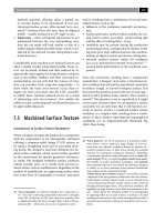
7.5 Machined Surface Texture
Introduction to Surface Texture Parameters
When a designer develops the features for a component
with the requirement to be subsequently machined

utilising a computer-aided design (CAD) system, or
by using a draughting head and its associated draw-
ing board, the designer’s neat lines delineate the de-
sired surface condition, which can be further specied
by the requirement for specic geometric tolerances.
In reality, this designed workpiece surface condition
cannot actually exist, as it results from process-in-
duced surface texture modications. Regardless of the
method of manufacture, an engineering surface must
have some form of ‘topography, or texture’ associated
41 ‘Servo-mismatch’ , can oen be mistaken for a ‘squareness er-
ror’ , but if the contouring interpolation direction is changed,
from G02 (clockwise) to G03 (anti-clockwise) rotation, then
an elliptical prole will ‘mirror-image’ (‘ip‘) to that of the op-
posite prole – which does not occur in ‘squareness errors’.
with it, resulting from a combination of several inter-
related factors, such as the:
•
Inuence of the workpiece material’s microstruc-
ture,
•
Surface generation method which includes the cut-
ting insert’s action, associated actual cutting data
and the eect of cutting uid – if any,
•
Instability may be present during the production
machining process, causing induced chatter, result-
ing from poor loop-stiness between the machine-
tooling-workpiece system and chosen cutting data,
•

Inherent residual stresses within the workpiece
can occur, promoted by internal ‘stress patterns’
42
–
causing latent deformations in the machined com-
ponent.
From the restrictions resulting from a component’s
manufacture, a designer must select a functional sur-
face condition that will suit the operational constraints
for either a ‘rough’ , or ‘smooth’ workpiece surface. is
then raises the question, posed well-over 25 years ago –
which is still a problem today, namely: ‘How smooth is
smooth?’ is question is not as supercial as it might
at rst seem, because unless we can quantify a surface
accurately, we can only hope that it will function cor-
rectly in-service. In fact, a machined surface texture
condition is a complex state, resulting from a combi-
nation of three distinct superimposed topographical
conditions (i.e. as diagrammatically illustrated Fig.
160a), these being:
42 ‘Stress patterns’ , are to be expected in a machined compo-
nent, where: corners, undercuts, large changes in cross-sec-
tions from one adjacent workpiece feature to another, etc.,
produce localised zones of high stress, having the potential
outcome for subsequent component distortion. ‘Modelling’
a component’s geometry using techniques such as: nite ele-
ment analysis (FEA), or employing photo-elastic stress analy-
sis* models or similar simulation techniques, will highlight
these potential regions of stress build-up, allowing a designer
to nullify, or at worst, minimise these potential undesirable

stress regions in the component’s design.
*Photo-elastic stress analysis displays a stress-eld, normally
a duplicate of the part geometry made from a thin two-dimen-
sional (planar) nematic liquid crystal, or more robustly from
a three-dimensional Perspex model, which is then observed
through polarised light source. is polarised condition, will
highlight any high-intensity stress-eld concentrations in the
part , which allows the ‘polarised model’ to be manipulated
by applying either an un-axial tension, or perhaps a bi-axial
bending external stress to this model, showing dynamically its
potential stress behaviour during its intended in-service con-
dition.
Machinability and Surface Integrity 
Figure 160. Surface texture comprises of: ‘long-’, ‘medium-’ and ‘short-components’, together with the
‘direction of the dominant pattern’ – superimposed upon each other. [Courtesy of Taylor Hobson]
.
 Chapter 
1. Roughness – comprising of surface irregularities
occurring due to the mechanism of the machining
production process and its associated cutting insert
geometry,
2. Waviness – that surface texture element upon
which roughness is superimposed, created by fac-
tors such as the: machine tool, or workpiece deec-
tions, vibrations and chatter, material strain and
other extraneous eects,
3. Prole – represents the overall shape of the ma-
chined surface – ignoring any roughness and wavi-
ness variations present, being the result of perhaps
the long-frequency machine tool slideway errors.

e above surface topography distinctions tend to be
qualitative – not expressible as a number – yet have
considerable practical importance, being an estab-
lished procedure that is functionally sound. e com-
bination of roughness and waviness surface texture
components, plus the surface’s associated ‘Lay’
43
are
shown in Fig. 160a. e ‘Prole’ is not depicted, as it
is a long-frequency component and at best, only its
partial aect would be present here, on this diagram.
e ‘Lay’ of a surface tends to be either: anisotropic,
or isotropic
44
in nature on a machined surface topog-
raphy. When attempting to characterise the potential
functional performance of a surface, if an anisotropic
‘lay-condition’ occurs, then its presence becomes of
vital importance. If the surface texture instrument’s
stylus direction of the trace’s motion over the assessed
topography is not taken into account, then totally mis-
representative readings result for an anisotropic sur-
face condition occur – as depicted in Fig. 160b. is
is not the case for an isotropic surface topography, as
relatively uniform set of results will be present, regard-
less of the stylus trace direction across the surface (i.e.
43 ‘Lay’ , can simply be dened as: e direction of the dominant
pattern’ (Dagnall, 1998).
44 ‘Anisotropic, or isotropic surfaces, either condition can be in-
dividually represented on all machined surfaces. Anisotropy,

refers to a surface topography having directional properties,
that is a dened ‘Lay’ , being represented by machined feed-
marks (e.g. turned, shaped, planed surfaces, etc.). Conversely,
an isotropic surface is devoid of a predominant ‘Lay’ direc-
tion, invariably having identical surface topography charac-
teristics in all directions (e.g. shot-peening/-blasting and, to a
lesser extent a multi-directional surface-milling, or a radially-
ground surface, etc.).
see Fig. 161a – for an indication of the various clas-
sications for ‘Lay’).
Returning once more to Fig. 160b, as the stylus
trace obliquity changes from trace ‘A’ , inclining to
-
ward trace ‘E’ , the surface topography when at ‘E’ has
now become at, giving a totally false impression of
the true nature of the actual surface condition. If this
machined workpiece was to be used in a critical and
highly-stressed in-service environment, then the user
would have a false sense of the component’s potential
fatigue
45
characteristics, potentially resulting in ei-
ther premature failure, or at worst, catastrophic fail-
ure conditions. In Fig. 162, the numerical data (ISO
1302:2001), has been developed to establish and de-
ne relative roughness grades for typical production
processes. However, some caution should be taken
when utilising these values for control of the surface
condition, because they can misrepresent the actual
state of the surface topography, being based solely on a

derived numerical value for height. What is more, the
‘N-number’ has been used to ascertain the arithmetic
roughness ‘Ra’ value – with more being mentioned on
this and other parameters shortly. e actual ‘N-value’
being just one number to cover a spread of potential
‘Ra’ values for that production process. Neverthe-
less, this single numerical value has its merit, in that
it ‘globally-denes’ a roughness value (i.e.‘Ra’) and
its accompanying ‘N-roughness grade’ , which can be
used by a designer to specify in particular a desired
surface condition, this being correlated to a specic
production process. e spread of the roughness for a
specic production process has been established from
experimental data over the years – covering the maxi-
mum expected ‘variance’
46
– which can be modied
45 ‘Fatigue’ , can be dened as: ‘e process of repeated load, or
strain application to a specimen, or component’ (Schaer, et
al., 1999). Hence, any engineering component subjected to
repeated loading over a prescribed time-base, will normally
undergo either partial, or complete fatigue.
46 ‘Variance’ , is a statistical term this being based upon the
standard deviation, which is normally denoted by the Greek
symbol ‘σ’. us, variance can be dened as: ‘e mean of the
squares of the standard deviation’ (Bajpai, et al., 1979).
us, σ = √Variance, or more specically for production op-
erations:

�

s 

n   
n

j=
x
j

¯
x

*s = the standard deviation of a sample from a production
batch run.
Machinability and Surface Integrity 
depending upon whether a ne, medium, or coarse
surface texture is obligatory. Due to the variability in
any production process being one of a ‘stochastic out-
put’
47
, such surface texture values do not reect the
likely in-service performance of the part. Neither the
surface topography, nor its associated integrity has
been quantied by assigning to a surface representa-
tive numerical parameters. In many instances, ‘surface
engineering’
48
is utilised to enhance specic compo-
nent in-service condition.
It was mentioned above that in many in-service

engineering applications the accompanying surface
texture is closely allied to its functional performance,
predominantly when one, or more surfaces are in mo-
tion with respect to an adjacent surface. is close
proximity between two mating surfaces, suggests that
the smoother the surface the better, but this is not nec-
essarily true if the surfaces in question are required to
maintain an ecient lubrication lm between them.
e apparent roughness of one of these surfaces with
respect to the other, enables it to retain a ‘holding-
lm’ in its associated topographical ‘valleys’
49
. While
another critical factor that might limit the designer’s
choice of the smoothness of an engineering surface’s
selection, is related to its production cost (i.e. see
Fig. 161b). erefore, if the designer requires a very
smooth machined surface, it should be recognised that
its manufacturing time is considerably longer – so its
respective cost will be greater to that of a rough sur-
face, this being exacerbated by a very close dimen-
sional tolerance requirement.
47 ‘Stochastic processes’ , are dened as: ‘A process which has a
measurable output and operating under a stable set of condi-
tions which causes the output to vary about a central value in a
predictable manner’ (Stout, 1985).
48 ‘Surface engineering’ , is applying suitable discrete technolo-
gies to create surface lms (e.g. 10 to 100 nm thick), or by ma-
nipulating the surface atomic layers (e.g. 2 to 10 atomic layers,
approximately 0.5 to 3 nm), to enhance the ‘engineered’ sur-

face condition (i.e. Source: Vickerman, 2000).
49 ‘Surfaces’ , are recognised to have topographical features that
mimic the natural world. So a regular/irregular engineering
surface can exhibit both peaks and valleys, not unlike moun-
tainous terrain.
.. Parameters for Machined
Surface Evaluation
In order that a machined workpiece’s surface texture
can be determined using stylus-based (two-dimen-
sional) instrumentation, three characteristic lengths
are associated with this surface’s prole (i.e. see
Fig. 163a), these are:
1. Sampling length
50
– is determined from: the length
in the direction of the X-axis used for identifying
the irregularities that characterise the prole under
evaluation. erefore, virtually all surface de-
scriptors (i.e. parameters) necessitate evaluation
over the sampling length. Reliability of the data
is enhanced by taking an average of the sampling
lengths as depicted by the evaluation length shown
in Fig. 162a. Most of today’s stylus-based surface
texture instruments undertake this calculation au-
tomatically,
2. Sampling length – can be established as: the to-
tal length in the X-axis used for the assessment of
the prole under evaluation. From Fig. 163a, this
length may include several sampling lengths – typi-
cally ve – being the normal practice in evaluating

roughness and waviness proles. e evaluation
length measurement is the sum of the individual
sampling lengths (i.e. it is common practice to em-
ploy a 0.8 mm sampling length for most surface
texture assessments),
3.
Traverse length – can be dened as: the total
length of the surface traversed by the stylus in mak-
ing a measurement. e traverse length will nor-
mally be longer than the evaluation length (i.e. see
Fig. 163a), this is due to the necessity of allowing
‘run-up’ and ‘over-travel’ at each end of the evalua-
tion length. ese additional distances ensure that
any mechanical and electrical transients, together
lter edge eects are excluded from the measure-
ment.
50 ‘Sampling length’ , is oen termed ‘Meter cut-o ’ , or simply
the ‘cut-o ’ length and its units are millimetres. e most
common cut-os are: 0.25, 0.8, 2.5, 8.0, 25.0 mm. e 0.8 mm
sampling length will cover most machining production pro-
cesses. In any surface texture evaluation, it is essential that the
cut-o is made known to the Inspector/Metrologist reviewing
this surface topographical data.
 Chapter 
e number of two-dimensional surface prole pa-
rameters that have been developed over the years for
just the stylus-based instruments – discounting the
three-dimensional contact and non-contact varieties,
has created a situation where many users simply do
not understand, nor indeed comprehend the intrinsic

dierences between them! A term was coined some
years ago to show exasperation by many metrolo-
gists’ with this ever-increasing development of such
parameters. Many researchers and companies were
totally disenchanted with their confunsion and plight,
so they simply called the predicament: ‘parameter-
rash’. However, here we need not concern ourselves
with this ‘vast expanse of surface descriptors’ , as only
a few of the well-established parameters and discuss
just the most widely-utilised ones. It is worth making
Figure 161. ‘Lay’ indicated on drawings, plus the relative cost of manufacture for dierent production processes.
Machinability and Surface Integrity 
Figure 162. Anticipated process ‘roughness’ and their respective grades. [Source: ISO 1302, 2001].
 Chapter 
Figure 163. Surface texture data-capture, with techniques for the derivation of the arithmetic roughness parameter: Ra.
Machinability and Surface Integrity 
the point, that all of these two-dimensional surface pa-
rameters can be classied into three distinct groupings
and just some of these parameters are:
1. Amplitude parameters (Ra, Rq, Wa, Wq, Pa, Pq)
51

– with Ra
52
being universally recognised for the
‘international’ parameter’ for roughness. It is: ‘e
arithmetic mean of the absolute departures of the
roughness prole from the mean line’ (i.e. see Fig.
163b and c). It can be expressed as follows:

Ra  lr
l r


 zx  dx
(units of m)
NB e Ra parameter is oen utilised in appli-
cations to monitor a production process, where a
gradual change in the surface nish can be antici-
pated, making it seem to be ‘ideal’ for any form of
machinability trials, but some caution is required
here, as will be seen shortly in further discussion
concerning this ‘surface descriptor’. By way of com-
parison, another previously used amplitude param-
eter is given in Appendix 10 and is the ‘R
Z
(JIS)’ (i.e.
10-point height) parameter.
Other useful parameters of the assessed prole, to be
shortly discussed in more detail, include: ‘Skewness’
(Rsk, Wsk, Psk), which is oen utilised in association
with ‘Kurtosis’ (Rku, Wku, Pku), producing the so-
called: ‘Manufacturing Process Envelopes’ – as a means
of ‘mapping’ and correlating machined surface topog-
raphies.
2. Spacing parameters (Rsm, Wsm, Psm) – can be de-
ned as: ‘e mean spacing between prole peaks at
the mean line, measured within the sampling length’
(i.e. depicted along a machined cusp – at diering
51 e designation of the letters follows the logic that the pa-

rameter symbol’s rst capital letter denotes the type of prole
under evaluation. For example, the: Ra* – calculated from the
roughness prole; Wa – derives its origin from the waviness
prole; with the latter in this logical sequence, namely the Pa
– being derived from the primary prole. Here, in this discus-
sion and for simplicity, only the rst term in the series – e.g.
‘Ra’ notation – will be used.
*Ra is today shown in the International Standard (i.e. ISO
4287: 1997) as being denoted in italics, while in the past, it was
usually shown as follows: ‘R
a
’ , but even now, many companies
still use this particular notation.
52 Historically, the classication of the relative roughness of sur-
faces was initially developed in England and was then termed:
‘Centre Line Average’ (CLA), while in the USA its equivalent
term was the ‘Arithmetic Average’ (AA).
feedrates in Fig. 169a and b). It can be expressed in
the following manner:

Rsm  n
i=n

i=
si 
XS+ XS+XS + XSn
n

Where:
n = number of peak spacings.

NB e Rsm parameter needs both height and spac-
ing discrimination and, if not specied the default
height bias utilised is 10% of: Rz, Wz, or Pz, – where
these are the ‘Maximum height of prole’. As can be
seen from the ‘idealised’ machined surface topog-
raphy given in Fig. 169a and b, the spacing param-
eters are particularly useful in determining the feed
marks. Moreover, the Rsm parameter relates very
closely to that of the actual programmed feed rev
–1
of
either the cutter, or workpiece – depending on which
production process was selected. See also, Appendix
10 for a graphical representation of the previously
utilised ‘High Spot Count’ (HSC) parameter.
3. Hybrid parameters (Rmr, Wmr, Pmr, R∆q, W∆q,
P∆q, Rpk, Rk, Rvk) – each of these ‘hybrids’ will
now be briey mentioned. Rmr, or its alternative
notation Mr is the ‘Material ratio curve’ , which can
be dened as: ‘e length of the bearing surface (ex-
pressed as a percentage of the evaluation length ‘L’) at
a depth ‘p’ below the highest peak (i.e. see Fig. 165).
–
Rmr:
It is oen known as the
‘Abbott-Firestone curve’ ,
the mathematics of this Rmr-curve can be ex-
pressed in the following manner:
 
Rmr 

b+b+b=B +bn
n
  

n
i=n

i=
bi
NB is ‘Material ratio curve’ represents the pro-
le as a function of level. More specically, by plot-
ting the bearing ratio at a range of depths in the
prole trace, the manner by which the bearing ratio
changes with depth, provides a method of charac-
terising diering shapes present on the prole (i.e.
see Fig. 165 and Appendix 10).
–
R∆q:
e
R∆q parameter, can be dened as: ‘e root
mean square (rms) slope of the prole within the
sampling length’ (i.e. see how its angle changes at
diering machining feedrate conditions shown
in Fig. 169b and c), it can be mathematically ex-
pressed as follows:
 Chapter 

R q 

lr

l r


θx
¯
θ

dx
Where:

¯
θ  lr
l r


θxdx
 
θ = slope of the prole at any given point.
•
Rpk, Rk, Rvk:
ese parameters (i.e. see Appendix 10 for graphi
-
cal representations of the parameters), were origi-
nally designed for the control of potential wear in
automotive cylinder bores in volume production
by the manufacturing industry. Today, Rpk, Rk and
Rvk are employed across a much more diverse-eld
by a range of industries. Such hybrid parameters
are an attempt to explain – in numerical terms, the
respective form taken from the prole’s trace of the

‘material ratio curve’ (Rmr), hence:
–
Rpk parameter – is the ‘reduced peak height’ , il-
lustrating that the top portion of a bearing sur-
face will be quickly worn-away when for exam-
ple, an engine initially begins to run,
–
Rk parameter – is known as the ‘kernal rough-
ness depth’ , therefore the long-term running –
‘steady-state wear’ of this surface will inuence
for example, the performance and life of the au-
tomotive cylinder(s),
–
Rvk parameter – is the ‘trough depth’ this in-
dicates that the surface topography has an oil-
retaining capability, specically via the ‘trough
depths’ which have been purposely ‘cross-
honed’
53
into the bore’s surface.
Arithmetic roughness parameter (Ra)
Although the Ra ‘amplitude parameter’ has been
widely quoted ‘Internationally’ , there are a few provi
-
53 ‘Cross-honing’ , uses either: (ne) Abrasives/CBN/Diamond –
‘stones’ , that are tted into a ‘honing head’ which then rotates
and oscillates within a hole, or an engine’s bore. e critical
parameters are the rotational speed (Vr) oscillation speed
(Vo), the length and position of the honing stroke, the hon-
ing stick pressure (Vc). e inclination angle of the cross-hon-

ing action, is a product of the up-/down-ward head motion
(Vo) and the rotational speed for the head (Vo). is complex
action of rotating and linear motion, generates the desired
cross-honed ‘Lay-pattern’ within the bore – for improved oil
retention.
sos, or conditions that must be met, if it is to be utilised
satisfactorily, these are:
•
e Ra value over one sampling length represents
the average roughness. e eect of a spurious non-
typical peak, or valley within the prole’s trace be-
ing ‘averaged-out’ so will have only a small inu-
ence on the Ra value obtained;
•
e evaluation length contains several sampling
lengths (Fig.163a), this ensures that the Ra value is
representative of the machined surface under test;
•
An Ra value alone is meaningless, unless quoted
with its associated metre cut-o (λc) length. Repeat-
ability of the Ra value will only occur at an identi-
cal length of metre cut-o;
•
If a dominant surface texture pattern occurs (Lay), then
the Ra readings are taken at 90° to this direction;
•
at Ra does not provide information as to the
shape of either the prole, or its surface irregulari-
ties. Dierent production processes generate diverse
surface nishes, for this reason its is usual to quote

both the anticipated Ra numerical value along with
the actual manufacturing process;
•
Ra oers no distinction between peaks and valleys
on the surface trace.
e most confusing argument concerning the use of
an Ra value alone, is that its numerical value is not
only meaningless, but it can have catastrophic conse-
quences if interpreted incorrectly. ese opinions can
be substantiated by close observation of Fig. 164a,
where an identical numerical Ra value produces
widely divergent surface topographies. In addition, if a
designer’s engineering application called for a ‘bearing
surface’ (Fig. 164ai), rather than a ‘locking surface’ (Fig.
164aiii), then the numerical value of 4.2
µm in isola-
tion, becomes pointless, as it tells the designer nothing
about the ‘functional’ surface topography. is prob-
lem is exacerbated when the wrong surface topography
is selected for a specic engineering application. For ex-
ample, a ‘locking surface’ applied to a bearing industrial
application in a harsh environment, can be expected to
catastrophically fail aer very little in-service time.
Skewness (Rsk, Wsk, Psk) and Kurtosis
(Rku, Wku, Pku) Parameters
ese surface descriptors of ‘skewness’ and ‘kurtosis’
are oen derided as simply ‘statistical’ amplitude pa-
rameters, that can introduce spurious results and as a
consequence, having little use in engineering applica-
tions. However, when used in the correct context, they

can provide a valuable insight into the overall shape of
Machinability and Surface Integrity 