Machining of High Strength Steels With Emphasis on Surface Integrity by air force machinability data center_10 ppt
Bạn đang xem bản rút gọn của tài liệu. Xem và tải ngay bản đầy đủ của tài liệu tại đây (778.49 KB, 9 trang )
bration certicate, to ensure that the results obtained
are both valid and sound. A cautionary note: if the dy-
namometer has been inadvertently dropped, or it has
possibly collided with an obstruction when in use on
the machine tool, it should be sent back to the manu-
facturer for servicing and recalibration, otherwise,
spurious cutting force data may be the result.
7.9 Machining Modelling
and Simulation
Introduction
Previously, it was been widely accepted that most cut-
ting tool modelling technqiues are somewhat incom-
plete, in both their analysis of the process and their
accompanying derived mathematics. Early, but worthy
attempts at analysing the chip formation mechanics of
the orthogonal cutting process were undertaken ini-
tially by Ernst and Merchant (1941) – shown schemat-
ically depicted in Fig. 181, followed by further work
concerning the analytical graphical interpretation of
the orthogonal cutting action which was presented
by Merchant and Zlatin (1945) and later work by Lee
and Shaer (1951) – not shown. is earlier work
was then followed by Zorev’s (1963) interpretation of
an ‘idealised cutting model’ (Fig. 182). In all of these
above modelling cases and others not mentioned – for
brevity’s sake!, the very complex nature of the cutting
process, is a vast subject ‘straddling’ many engineering
and physical disciplines. Such modelling involves as-
pects of: the tool’s geometry, chip/tool contact lengths
and pressures, chip formation, cutting forces, fric-
tional and thermal factors and so on, making it vir-
tually impossible to obtain close agreement between
with any truly meaningful results between each pro-
posed model. is lack of correlation of these model-
ling processes, is to be expected, as in reality a shear
zone, rather than a shear plane exists, but for mathe-
matical treatment, a shear plane allows some degree of
geometrical association. Due to the complex nature of
the inter-related variables that occur in any dynamic
cutting situation for just simply the orthogonal cutting
process, let alone for oblique machining modelling,
this has meant that the ‘optimum modelling solution’
has as of now, not yet been fully addressed.
Many ‘learned tomes’ have been written in the past,
concerning the ‘mechanics of machining’ and it is not
the intention to fully discuss them here, in this book
which is principally concerned with ‘current practice’
concerning machining applications. However, a brief
resumé of just one of these ‘orthogonal models’ shown
in Fig. 181 will be mentioned below, together with a
concise review of friction in metal cutting operations
(Fig. 182) will be presented, to attempt to show why
the subject of ‘theoretically modelling’ the cutting pro-
cess is so complicated.
Ernst and Merchant’sComposite Cutting Force Circle
If a continuous chip formation is produced when ma-
chining ductile materials in an orthogonal cutting
process, such as that found when cylindrically turn-
ing a component’s periphery with an undeformed chip
thickness (‘t
1
’), this will cause a chip compression (‘t
2
’)
– Fig. 181(top). e cutting forces can be obtained by
employing a cutting force dynamometer as discussed
in the previous section, to typically measure the forces
‘F
C
’ and ‘F
T
’ and so on. By utilising such cutting tool
dynamometry, Ernst and Merchant (1941) were able
to classify the forces acting in the vicinity of metal cut-
ting which gave rise to both local plastic deformation
and frictional eects. In Ernst and Merchant’s theory
which is oen termed the so-called ‘shear-angle solu-
tion’ , it is assumed that the cutting edge is always per-
fectly sharp and that a continuous-type chip without
BUE occurs, this former assumption in practice does
not actually occur. Moreover, another assumption in
their analysis it was that the chip would behave like
a ‘rigid body’ , which is held in equilibrium by the ac
-
tion of the applied forces transmitted across the tool/
chip interface and transversely over the shear plane.
Boothroyd (1975), oered a reasonably ‘elegant solu-
tion’ to Ernst and Merchant’s numerical and geometri-
cal analysis and, this has been somewhat modied and
further simplied below. In order to abridge the ‘shear-
angle solution model’ shown in Fig. 181, the resultant
force ‘R’ is depicted acting at the tool’s cutting edge,
being resolved into components ‘N’ and ‘F’ in direc-
tions along and normal to the tool’s face respectively,
as well as into components ‘F
N
’ and ‘F
S
’ – once again,
along and normal to the shear plane correspondingly.
Further, the cutting force ‘F
C
’ and the thrust ‘F
T
’ com-
ponents of the resultant force, are also shown. Here, it
can also be assumed that the entire resultant force is
transmitted across the tool/chip interface and that on
both the tool’s ank and edge no force occurs, mean-
ing that a zero ‘ploughing-force’ is present – see Fig.
184 which illustrated this ‘nose-rounding eect’.
Chapter
e foundation purported by Ernst and Merchant’s
theory, was the proposition that the shear angle ‘φ’
would acquire such a value, thereby reducing the ac-
tual work done to a minimum. In view of the fact that
that for preselected cutting conditions, the work done
during cutting was comparative to that of ‘F
C
’ in terms
of ‘φ’ , hence allowing one to obtain the value of ‘φ’
when ‘F
C
’ is at a minimum. us, from Fig. 181:
Figure 181. ‘Merchant’s’ composite metal cutting circle for an orthogonal cutting model, where:
• F
T
= thrust force component,
• F
C
= cutting force component,
• F
N
= normal force component on the shear plane,
• F
S
= shear force component on shear plane,
• R = resultant tool force component,
• N = normal force component on tool face,
• Φ = shear angle,
• α = working normal rake angle,
• τ = mean friction angle on tool face,
• t
1
= undeformed chip thickness,
• t
2
= deformed/compressed chip thickness,
• A
0
= cross-sectional area of uncut chip,
• A
c
= cross-sectional area of deformed/compressed chip.
NB: Force arrow vector directions have been reversed and some terms have been modied from the original
work. [Source: Ernst & Merchant, 1941]
.
Machinability and Surface Integrity
F
S
= R cos(φ + τ – α) (i)
and
F
S
= τ
S
A
S
= τ
S
A
C
/sin φ (ii)
Where:
τ
S
= Workpiece material’s shear strength – on the
shear plane,
A
S
= Shear plane’s area,
A
C
= Uncut chip’s cross-sectional area,
τ = Mean friction angle, between too and chip [i.e.
arctan (FT/FN)],
α = Normal rake angle (i.e. working).
From equations (i) and (ii):
R =
τ
s
A
c
sin ϕ
cos(ϕ + τ − α)
(iii)
By geometry:
F
C
= R cos(τ – α) (iv)
Hence, from equations (iii) and (iv):
F
c
=
τ
s
A
c
sin ϕ
cos(τ − α)
cos(ϕ + τ − α)
(v).
Now, equation (v) can be dierentiated with respect
to ‘φ’ , then equated to zero to obtain a value of ‘φ’
when ‘F
C
’ is at a minimum. Hence, the requisite value
is specied by:
ϕ + τ − α =
π
(vi).
In comparative analysis undertaken by Merchant
(1945), he found close correlation with experimental
results was obtained when machining synthetic plas-
tics, but a somewhat poor theoretical correlation oc-
curred when steel had been machined with cemented
carbide tooling. It needs to be mentioned that when
Merchant dierentiated with respect to ‘φ’ , it was as-
sumed that ‘A
C
’ , ‘α’ and ‘τ
S
’ would be independent of
‘φ’ , but on further consideration, Merchant decided to
oer in a ‘modied theory’ the relationship of :
τ
S
= τ
So
+ kσ
S
(vii).
Here, Merchant brought in a modication to the shear
strength of the workpiece material ‘τ
S
’ which now in-
creased linearly with an increase in normal stress ‘σ
S
’
on the shear plane, where zero normal stress ‘τ
S
’ is
equal to ‘τ
So
’. is new assumption by Merchant was
conrmed by previous work undertaken in the litera-
ture published by Bridgman (1935, ’37 and ’43), where
the shear strength when experimental machining of
polycrystalline metals was shown to be dependent on
the normal stress on the ‘plane of shear’.
Now from Fig. 181, we can obtaing the following
relationship:
F
Ns
= F sin(φ + τ – α) (viii)
and:
F
Ns
= σ
S
A
S
=
σ
S
A
C
sin ϕ
(ix).
From equations (viii) and (ix):
σ
S
=
sin ϕ
A
C
R sin(ϕ + τ − α)
(x).
Combining equations (iii) and (x):
τ
S
= σ
S
cot(φ + τ – α) (xi)
and, from equations (vii) and (xi):
τ
S
=
τ
So
− k tan(ϕ + τ − α )
(xii).
is equation (i.e. xii), explains why the value of ‘τ
S
’
may be inuenced by modications in the shear angle
(‘φ’), which is now inserted into equation (v), to ob-
tain a new equation for ‘F
C
’ in terms of ‘φ’ , therefore,
the resulting expression becomes:
F
C
=
τ
So
A
C
cos(τ − α)
sin ϕ cos(ϕ + τ − α)[ − k tan(ϕ + τ − α)]
(xiii).
Now, it can be assumed that both ‘k’ and ‘τ
So
’ are con-
stants for the specic workpiece material, further, that
‘A
C
’ and ‘α’ are also constants for the machining op-
eration. Hence, equation (xiii) can now be dierenti-
ated to obtain a new value of ‘φ’ , with the resulting
expression:
2φ + τ – α = C
Where:
C = Can be obtained from ‘arccotk’ , which is a con-
stant for the workpiece material.
NB In further more recent experimental work, it has
been shown that ‘τ
S
’ will remain constant for a speci-
ed workpiece material, across a diverse range of cut-
Chapter
ting conditions, as such, the value of ‘k’ can be equated
to zero.
When the shear-angle values are compared for the
plotted linear relationships of the earlier theoretical
and experimental work undertaken by Ernst and Mer-
chant, to that of the later comparative work by Lee and
Shaer, then these shear-angle relationships diverge
somewhat. However, one area that these researchers
both agreed upon, was the fact that friction on the
tool’s face was the most important factor during metal
cutting. In the following discussion, the inuence that
frictional behaviour has at the tool/chip interface will
be briey mentioned.
Frictional Effects During Machining
For simplicity’s sake, friction between dry sliding sur-
faces will be concisely reviewed. In 1699 Amontons
‘laws of friction’
78
were formulated, then veried by
Coulomb
79
in 1785, with Bowden and Tabor (1954)
contributing greatly to an explanation of these empiri-
cal laws.
If two apparent at surfaces are placed together, the
larger asperities (i.e. peaks) on each mating face will
only establish contact. With just normal loading, the
top of these asperities will yeild, creating a real area
of contact until such a time, that they are capable of
supporting an applied load. In the main, for the vast
majority of engineering applications this real contact
area (‘A
r
’), is normally only a very minute portion of
the apparent real of contact (‘A
a
’) – even aer the con-
tacting asperities of the soer material has plastically
deformed (i.e. yielded). us:
A
r
= F
n
/σ
y
(i)
78 ‘Law(s) of friction’ , Amontons in 1699 stated in the main,
that: ‘Friction is independent of the apparent area of contact
and proportional to the normal load between two [mating] sur-
faces.’
79 Coulomb (1785), conrmed these ‘frictional laws’ with the
observation that: ‘e coecient of friction* is substantially in-
dependent of the speed of sliding.’
*Coecient of friction (µ) = F/N
us, the friction force is proportional to the perpendicular
force between contacting surfaces and is independent of the
surface area, or its ‘rubbing speed’.
Where:
F
n
= Normal force,
σ
y
= Yield pressure of the soer material.
us, for most metallic materials, this close asperity
contact between mating surfaces creates localised ‘cold
welding’. Prior to any sliding with respect to these two
contacting surfaces, a force is necessary to continually
shear potentially contacting and reforming asperity
tips of these ‘welded junctions’. Hence, the total fric-
tional force ‘F
f
’ is given by:
F
f
= τ
f
A
r
(ii)
Where:
τ
f
= Shear strength of soer contacting material,
A
r
= Real contact area.
From equations (i) and (ii), the actual coecient of
friction (‘µ’) between these contacting surfaces will
be:
µ = F
f
/F
n
= τ
f/
σ
y
(iii).
In majority of machining operations typied by the
continuous turning of metallic workpieces, the coef-
cient of friction (‘µ’) at the chip/tool interface can
vary quite considerably. Its frictional variation, being
inuenced by any changes in: cutting speed, feedrate,
rake angle contact regions – this latter factor is par-
ticularly relevant for multi-functional tooling, where
the cutting insert’s top face is not planar (i.e at). In
modern machining practice, the normal pressures ex-
erted at the tool/chip interface are exceedingly high,
typically when machining commercial grades of me-
dium carbon plain steels these pressures are >3.5 GPa.
is high normal pressure at the ‘interface’ causes the
real contact area to approach that of the entire area,
where: A
r/
A
a
= unity! is means that under these cir-
cumstances the ordinary laws of friction no longer ap-
ply, and the frictional force ‘F
f
’ is still represented by
equation (ii), but is now independent of the normal
force ‘F
n
’. is acute change in the frictional behaviour
during machining, means that the shearing action is
not conned only to the interface asperities, but in-
cludes workpiece material in the local substrate.
In work published by Zorev in 1963, his ‘model’
considered the frictional behaviour in continuous
metal cutting operations where no BUE was present
(Fig. 182). Under these machining conditions, Zorev
Machinability and Surface Integrity
noted that the normal stresses at the tool/chip inter-
face were suciently high enough to cause ‘A
r/
A
a
’ to
approach unity, over the zone denoted given by length
‘l
st
’ (Fig. 182) – this being termed the ‘sticking region’
80
– also see magnied quick-stop photomicrograph in
Fig. 184(top) showing the aect on the resultant chip.
e ‘sliding region’ , extends from from the end of the
‘sticking region’ to a point where the chip loses contact
with the rake face (i.e. ‘l
f
’-‘l
st
’), here, the ‘A
r
/A
a
’ ratio is
less that unity – meaning that the coecient of friction
is constant. In 1964, Wallace and Boothroyd produced
evidence that the ‘sticking manner’ observed on the
underside of the chip had abruptly stopped. ey ob-
served that in an adjacent vicinity to that of the tool’s
cutting edge, grinding marks on the rake face were im-
printed onto the chip’s underside. is phenomenon
indicated that no relative motion between the chip and
the tool had occurred, suggesting that here, the ‘real’
and ‘apparent’ areas of contact were ‘equalised’ in this
region. erefore, under ‘sticking friction’ conditions,
the ‘mean angle of friction’ on the rake face, depends
on the:
1. Form of the normal stress distribution,
2. Tool/chip contact length (i.e. ‘
l
f
’),
3. Mean shear strength of the chip material – in the
‘sticking region’ ,
4. Coecient of friction – in the
‘sliding region’.
NB It seems apparent that a simple numerical value
for the mean angle of friction, is inadequate when at-
tempting to completely describe the frictional circum-
stances on the rake face.
In Fig. 182, is schematically depicted the ‘frictional
model’ purported by Zorev (1963). Here, Zorev sug-
gested that the normal stress distribution (‘σ
f
’) on the
tool’s rake face, could be represented by the following
simple expression:
σ
f
= qx
y
(iv)
80 ‘Sticking region’ at the tool/chip interface is oen termed the
‘stagnation zone’ , but in this case it appears on the formed/
sheared chip – depicted in Fig. 184 (top). Here, is shown a
magnied and etched view of a quick-stop for an insert cut-
ting carbon steel at 150 m min
–1
. A ‘stagnation zone’ is present,
that follows the insert’s prole, with ‘soened’ workpiece ma-
terial protecting the tool, by a sticking/sliding action. A ‘ow
zone’ occurs aer ‘shear plane’ , visibly dividing undeformed/
deformed material.
Where:
‘x’ = Distance along the rake face – from the
position where the chip losses contact with the tool’s
face,
‘q’ and ‘y’ = are constants.
e maximum normal stress ‘σ
fmax
’ occurs when ‘x’
equals ‘l
f
’ , so:
σ
fmax
= ql
f
y
or, transposing with respect to ‘q’:
q = σ
fmax
l
f
–y
(v).
Substituting for ‘q’ in equation (iv), we get:
σ
f
= σ
fmax
(x/l
f
)
y
(vi)
us, in the ‘sliding region’ , ranging from: x=0 to
x = l
f
– l
st
the coecient of friction ‘µ’ is constant and,
the distribution of shear stress ‘τ
f
’ along this region, is
represented by:
τ
f
= σ
f
µ = µ σ
fmax
(x/l
f
)
y
(vii).
So, in the ‘sticking region’ , the shear stress becomes a
maximum (‘τ
st
’), therefore from: x= l
f
– l
st
to x=l
f
:
τ
f
= τ
st
(viii).
By integrating equation (vi) to obtain the normal force
‘F
n
’ acting on the rake face (i.e. from Fig. 181), gives:
F
n
a
w
l
f
σ
f m ax
xl
f
y
dx
= σ
fmax
a
w
l
f/
1 + y (ix)
Where:
a
w
= Chip width (i.e. width of cut).
e friction force ‘F
f
’ on the tool’s rake face, is ob-
tained by:
F
f
a
w
τ
st
l
st
l
f
−l s t
µ σ
f m ax
xl
f
y
dx
= τ
st
a
w
l
st
+ µ σ
fmax
a
w
(l
f
– l
st
)
1+y/
l
f
y
(1+y) (x).
At position: ‘x = l
f
-l
st
’ , the normal stress ‘σ
f
’ is given by:
‘τ
st
/µ’. Moreover, from equation (vi), it is given by:
Chapter
σ
fmax
(l
f
-l
st
/l
f
)
y
erefore:
τ
st
= µ σ
fmax
(l
f
– l
st
/l
f
)
y
(xi).
By substituting equation (xi) in equation (x), it simpli-
es the expression for ‘F
f
’ , as follows:
F
f
= τ
st
a
w
l
st
+ τ
st
a
w
(l
f
– l
st
)/1+y (xii).
Hence, the mean coecient of friction on the rake face,
can now be found from both equations (ix) and (xii):
Mean friction angle =
F
f
/F
n
= τ
st/
σ
fmax
(1+yl
st
/l
f
) (xiii).
From equation (xi), the mean normal stress on therake
face (σ
fav
) is given by:
σ
fav
= F
n
/a
w
l
f
= σ
fmax
/1+y
us:
σ
fmax
= (1+y)σ
fav
(xiv).
Substituting for ‘σ
fmax
’ in equation (xiii), produces:
Mean friction angle = arctan{
τ
st
/σ
fav
[1+y(l
st
/l
f
)]} (xv).
However, from Zorev’s experimental work, he found
that the term:
τ
st
[1+y(l
st
/l
f
)]/1+y
will remain relatively constant for a specied work-
piece material, across a diverse range of unlubricated
cutting conditions and, as a result, the equation for the
mean friction angle becomes:
Mean friction angle = arctan
K/σ
fav
(xvi)
Where:
‘K’ = a constant.
What Zorev’s equation (xvi) indicates, is that the mean
friction angle is somewhat dependent on the mean
normal stress on the rake face, allowing the result to
explain the eect of modications in the working nor-
mal rake to that of the mean friction angle. us, as the
value of ‘α’ (i.e. working normal rake angle) increases,
the resultant component tool force being normal to
the rake face will decrease, so that the mean normal
stress will be reduced. Moreover, from equation (xvi),
an increase in ‘α’ could be expected to increase the
mean friction angle. is observation, has been con-
rmed by experimental work undertaken by Pugh
(1958), where an increase in ‘α’ was shown to result in
a a complementary increase with repect to the mean
friction angle – across an extensive range of workpiece
materials.
Since the passage of time when both of these ‘theo-
retical models’ for the mechanics of machining and the
frictional work produced by Ernst and Merchant and
that of Zorev, respectively, were produced. Consider-
able eort and progress has been made into advances in
our present understanding of: ‘slip-line eld modelling’ ,
‘thermal and frictional modelling of the cutting process’ ,
‘chip-ow analysis’ , ‘examination of the primary and
secondary shear zones’ , non-orthogonal (three-dimen-
sional) machining processes, advances in tool geometries
with their accompanying force and shear relationships
and the advent of applications to machining opera-
tions employing nite element analysis (FEA). If all of
these subjects and other not listed, were only concisely
mentioned, then the book would be of epic propor-
tions! defeating the object of reviewing cutting appli-
cations and trends in current practice. However, the
role of FEA, in both machining research and for the
‘dynamic and geometric modelling’ of applied residual
stresses occurring in both the tool and workpiece in
the anticipated cutting processes is worthy of discus-
sion. e topic of ‘computer simulation’ utilising an
FEA approach, has become of increasing importance
of late and several companies have produced products
in this eld. However, to obtain some degree of con-
sistency in the dialogue only one particular company’s
FEA product will now be described.
Computer Simulation of Machining
Processes – an Introduction
By the application of computers to simulate and anal-
yse machining processes, this provides tool manufac-
turers and users alike, assistance in improving machin-
ing eciency and will also predict the likely cutting
response to real-time machinability environments.
Most of the early two-dimensional simulation models
for the mechanics of machining, focussed attention on
shear-zone modelling. ese previous ‘models’ ignored
vital factors such as the frictional conditions along and
between the rake’s tool/chip interface, furthermore,
any potential work-hardening and temperature eects
in this vicinity were also tended to be disregarded.
Machinability and Surface Integrity
Over the last two decades, the application of nite ele-
ment analysis (FEA) to that of three-dimensional ma-
chining applications, has been successfully applied to
the cutting process. Major advantages of using FEA,
are its ability to accurately compute: complex material
property denitions; tool/chip interactions; non-linear
geometric boundary conditions – typied by the chip’s
surface; prediction of local variables – such as stress
and temperature distributions in the cutting locality.
Several approaches for the numerical modelling
of machining operations and in particular, for that of
metal cutting have been employed, such as ‘Lagrang-
ian and Eulerian’ techniques. In the former case which
has been utilised for over two decades, ‘Lagrang-
ian methods’ utilise the tracking of discrete material
points. Here, the technique is uses a predetermined
line of separation at the tool’s point, which propagates
a ctitious crack ahead of the tool’s tip. Previously, this
Figure 182. An idealised orthogonal cutting model of chip-tool friction, where:
• σ
f
= normal stress,
• τ
f
= shear stress,
• τ
st
= shear strength of chip material in the sticking region,
• I
f
= chip-tool contact,
• I
st
= length of sticking region.
[Source: Zorev, 1963]
.
Chapter
routine precluded the resolution of the cutting edge
radius and an accurate resolution of the secondary
shear zone – due to severe mesh distortion. In an at-
tempt to alleviate any form of element mesh distortion
‘adaptive remeshing techniques’ have been employed
to resolve the tool’s cutting edge radius. Whereas the
‘Eulerian approach’ tracks volumes rather than mate-
rial particles, having the advantage of not needing to
rezone any distorted meshes. Moreover the ‘Eulerian
technique’ , requires ‘steady-state free-surface tracking
algorithms’ and relied upon a particular bur unrea-
sonable assumption that a uniform chip thickness oc-
curred, further this method precluded the modelling
of either a segmented chip formation, or that of the
milling process. e former technique of a ‘Lagrangian
FEA machining model’ will be reviewed (Fig. 183), as it
has the integrating ability to achieve ‘adaptive remesh-
ing’ with explicit dynamics and tightly coupled tran-
sient thermal analysis, allowing it to ‘model’ the com-
plex interactions between the cutting tool’s geometry
and that of the workpiece.
Lagrangian FEA Simulation
Machining Modelling
In Fig. 183, just a few images of the Lagrangian FEA
machining model are depicted for several applica-
tions of machining operations. is simulation mod-
elling technique contains a tightly coupled thermo-
mechanical material response capability, this being a
vital factor for any elevated temperatures that occur
at the tool/chip interface, furthermore, having a fully
adaptive mesh generation ability. Hence, the material
modelling facility forms an intergral part when at-
tempting to predict the workpiece’s material behav-
iour, under high strain and increased stress condi-
tions. is advanced modelling capability ensures the
accurate capture of any strain-hardening, or thermal
soening eects coupled to rate sensitivity properties,
for a given set of material conditions. Many of today’s
ferrous and non-ferrous materials, together with ‘ex-
otic materials’ such as nickel and titanium alloys can
also be successfully simulated, across a diverse range
of single- and multi-point cutting tools (e.g. turning,
milling, drilling, broaching, sawing, etc.).
Machining Simulation – Validation
Not only can simulation techniques of the type shown
in Fig. 183 be utilised for workpiece material machin-
ing modelling: work-hardening; thermal-soening
eects; machining-induced residual stresses; induced
temperature eects and heat-ow analyses with the
‘adaptive’ ‘Lagrangian FEA machining model’. e
‘model’ can also reasonably accurately predict: both
two- and three-dimensional cutting force magnitudes.
Invariably, the individual cutting force components
can be closely validated to actual machining working
practice, the same can also be said for a comparison
of a ‘dynamically-modelled chip’ to that of an actual
chip’s morphology – including both its chip-curling
tendency and any chip segmentation occurring. ese
validated simulation capabilities enable the cutting
process to be improved, by using the:
•
Force and temperature information – to reduce
overall production cycle times,
•
Temperature and thermal eects – can be utilised
to improve tool life and part quality,
•
Tool wear analysis – predicts the eects of tool
ank wear and how this wear land inuences sub-
sequent: temperatures, pressures and forces,
•
Chatter and vibration prediction – indicating the
onset and magnitude of these unwanted eects,
•
Residual stress information – helps alleviate poten-
tial machined component fatigue and aids in part
deformation analysis.
NB e inuence that tool coatings have on the
dynamic machining eciency can also be reviewed,
plus the capability to customise the tooling with
chip-breakers to improve chip-curl, or chip evacu-
ation abilities.
Computer machining simulation of the type illus-
trated in Fig. 183, can be integrated into an overall
CAD/CAM package, enabling a range of signicant
advantages to accrue, without having to operate a
costly and time-consuming task of undertaking an
extensive machinability trial. is o-line machining
simulation facility, allows: realistic cycle-time calcula-
tions including cut-and non-cut timings; visualisation
of tool paths to high-light and then avoid any localised
‘power-spikes’ occurring during a machining opera-
tion and many other useful production features.
e use of a dynamic FEA machining simulation
package similar to the one mentioned and illustrated
in Fig. 183, adds a scientic element to the understand-
ing of the overall machinability of specic workpiece
materials and associated tooling. Such machining
simulation oers not only a visual interpretation to
Machinability and Surface Integrity
Figure 183. Simulated machining processes. [Courtesy of Third Wave Advant Edge].
Chapter