Báo cáo hóa học: " Research Article Computational Issues Associated with Automatic Calculation of Acute Myocardial Infarction Scores" doc

Hindawi Publishing Corporation
EURASIP Journal on Advances in Signal Processing
Volume 2008, Article ID 670529, 10 pages
doi:10.1155/2008/670529
Research Article
Computational Issues Associated with Automatic Calculation
of Acute Myocardial Infarc tion Scores
J. B. Destro-Filho, S. J. S. Machado, and G. T. Fonseca
Biomedical Engineering Laboratory (BioLab), School of Electrical Engineering (FEELT), Federal University of Uberlandia (UFU),
Avenida Joao Naves de Avila 2121, Campus Santa M
ˆ
onica, 38400-902 Uberl
ˆ
andia, MG, Brazil
Correspondence should be addressed to J. B. Destro-Filho,
Received 2 December 2007; Revised 2 June 2008; Accepted 16 July 2008
Recommended by Qi Tian
This paper presents a comparison among the three principal acute myocardial infarction (AMI) scores (Selvester, Aldrich,
Anderson-Wilkins) as they are automatically estimated from digital electrocardiographic (ECG) files, in terms of memory
occupation and processing time. Theoretical algorithm complexity is also provided. Our simulation study supposes that the ECG
signal is already digitized and available within a computer platform. We perform 1000 000 Monte Carlo experiments using the
same input files, leading to average results that point out drawbacks and advantages of each score. Since all these calculations do
not require either large memory occupation or long processing, automatic estimation is compatible with real-time requirements
associated with AMI urgency and with telemedicine systems, being faster than manual calculation, even in the case of simple
costless personal microcomputers.
Copyright © 2008 J. B. Destro-Filho et al. This is an open access article distributed under the Creative Commons Attribution
License, which permits unrestricted use, distribution, and reproduction in any medium, provided the original work is properly
cited.
1. INTRODUCTION
In 2004, AMI was responsible for 22.93% of deaths associated
with cardiovascular diseases, which represents 6.39% of the

total number of deaths in Brazil [1]. In the United States [2],
coronary heart disease accounted for 489,171 deaths in 1990.
In consequence, AMI may be considered a public health
affair.
Current medical protocols require that, for AMI diagno-
sis, the patient should present at least two of the following
symptoms [3, 4].
(S1) chest pain;
(S2) specific ECG-waveform changements, particularly
ST elevation and/or ST depression;
(S3) high concentration of biochemical markers associ-
ated with the cardiac muscle necrosis, for example,
the concentration of enzymes Troponin and CK-
MB, which may be evaluated by means of blood
examinations.
Notice that, from (S1)–(S3), the last symptom is the most
important condition for assuring AMI diagnosis, and may
also be used as a relevant indicator of the injured myocardial
area, pointing out possible therapeutic procedures. However,
unconventional symptoms may be present in the patient [5].
In addition, detection of elevations on the concentration of
biochemical markers in the human plasma is not instanta-
neous, taking some time after the necrosis [3]. Such detection
also requires several hours to be completed [6] due to the
biochemical processes associated with this examination. In
consequence, based on (S2), ECG still remains the major tool
for speeding up AMI diagnosis, leading to the choice of the
treatment to be applied [6]. The costs of ECG are lower than
those associated with biochemical markers examination. One
should also point out that ECG is noninvasive and simple,

which explains its regular use, especially during the first
hours after the patient arrival to the hospital, as well as
during the monitoring of the AMI clinical evolution.
ECG-based diagnosis of AMI is successful for about 80%
of the cases [7, 8]. A recent consensus conference [3, 4, 6],
organized by the Joint Committee of the European Society
of Cardiology and the American College of Cardiology, has
reinforced the usefulness of the ST segment for this purpose.
For such diagnosis, ST elevation must appear in two or
more adjacent leads, presenting amplitudes higher than two
2 EURASIP Journal on Advances in Signal Processing
millimeters for leads V1–V3; or higher than one millimeter
for the other leads. These values suppose measurements
taken at the J point. In addition, the sum of ST elevations
considering all leads may be associated with the ischemic
acuteness of the cardiac tissue lesion, whereas other studies
point out that the number of leads presenting ST elevation
may be related to the extent of the injured area [9, 10].
ST-segment changements may be also used as a parameter
for assessing the effects of AMI treatments. In fact, the
literature [3, 8, 9, 11] reports decrease of ST-elevation after
the treatment.
Nevertheless, there are several other clinical issues and
pathologies leading to ECG-waveform changements, par-
ticularly regarding the ST segment, such as bundle branch
block, pacemakers [9], instrumentation, and heart rate
variability [8]. Despite these limitations, ECG analysis may
be considered until now the most simple, low cost, and
widespread means to evaluate and provide diagnosis on
cardiac ischemias [12]. It may also be useful to assess the

effects of therapies and to locate occlusions [7]. Based on the
ideas presented in [9, 10], several different indices have been
developed and tested by the literature, in order to further
extract useful information from the ECG, so that to speed up
diagnosis. These indices are based on specific morphologies
of the ECG during AMI, as disscussed below [12].
The Selvester score was created in 1972 by Selvester et al.
[13], which focuses the analysis on the QRS complex. It
is based on 57 criteria, considering all the leads (see the
Selvester table in Tabl e 6 ), summing up to 32 points. Each
point is physiologically equivalent to the necrosis of 3% of
the left ventricle, thus providing the estimation of the total
injured area by the AMI [13]. A simplified version of this
score was developed in 1982 by [14], including 37 criteria
and 29 total number of points, which was experimentally
validated. This score was thoroughly tested, providing a tool
with high specificity. During the chronic phase of the AMI,
this score is inversely proportional to the ejection fraction
(EF) of the left ventricle and directly proportional to the
dimension of the injured area [14].
The Aldrich score was developed in 1988 [15], aiming
at the estimation of the myocardial area under potential
risk of necrosis in the future, based on ECGs taken no later
than eight hours after the beginning of the infarction. The
calculation considers just ST-segment elevation/depression
in all leads, particularly the sum of all elevations (considering
all leads) and the number of leads associated with ST
elevation/depression. The reference for such measurements
is taken with respect to the J point, and equations depend on
the location of the AMI. Subsequent works in the literature

[16, 17] modified the original proposition by including other
parameters. It must be pointed out that the Aldrich score
performance decreases for patients undergoing thrombolytic
therapy [8, 11, 12, 16–18].
The Anderson-Wilkins score evaluates the time delay
between coronary occlusion and the patient first aid by
medical services [12, 19]. Such time delay is generally known
as “ischemic time,” which may be considered as a benchmark
for assessing the AMI acuteness, as well as the percentage
of the myocardial tissue which may be recovered by the
subsequent application of reperfusion therapy. It should be
pointed out, however, that the beginning of AMI symptoms
reported by the patient may be unaccurate, since atypical
AMIs may not lead to pain [5, 19
]. The Anderson-Wilkins
score classify the ECG waves in four types, based on an
analysis of the QRS complex and the T wave [12, 18–21].
These types indicate the degree of time evolution of the
ischemia. Although the original version of the Anderson-
Wilkins score presented different performances for anterior
and inferior AMI, a recent work in the literature [18]has
modified the equations, so that to overcome this drawback.
It is necessary to summarize information and compare
these scores. In fact, since QRS waveform changements take
place just in more advanced steps of the AMI process, and
since these changements are related to myocardial necrosis,
the Selvester score aims at estimating the percentage of
the myocardial area which has already been injured by the
AMI. On the other hand, since the ST elevation/depression
is related to the ischemic process without necrosis, the

Aldrich score may be considered as an estimator of the
myocardial area under the risk of future necrosis, as the
AMI evolves without treatment. Finally, Anderson-Wilkins
score analyzes two different classes of ECG elements: earlier
waveform changements (such as ample T waves and ST
depression/elevation), and delayed changements (such as the
pathological Q wave). In consequence, this score points out
the degree of time evolution of the AMI, putting forward the
time limit for the medicine to start reperfusion therapy.
In the literature, the classical procedure for score calcu-
lation is based on the visual inspection of the ECG, followed
by manual measurements with a ruler, which provides the
final quantities in millimeters to be applied in mathematical
expressions. This process is of course cumbersome, lengthy,
and subject to errors, which may introduce delays and
unaccuracy in the medical decision.
The clinical performance of these scores has been
assessed since the 1980s by several works of the literature.
Although they are not already used daily by cardiologists,
Aldrich and Anderson-Wilkins scores may be considered
those with the highest applicability. The first score is able to
put forward the acuteness of the AMI, which in turn helps the
decision on the therapy to be used and to establish prognosis
on the evolution of the patient clinical situation. On the
other hand, the second score points out the degree of time
evolution of the AMI, which is quite important to identify
patients to whom reperfusion procedure is still feasible and
efficient. Selvester score, though being studied since the
1980s and considered as a benchmark, may not be used at
the early stages of the patient care. This score supposes that

the AMI has already injured the heart. Consequently, if the
medicine evaluates the difference between the myocardial
area under the risk of injury, which is pointed out by the
Aldrich score; and that one which was already damaged, as
indicated by the Selvester score; it is possible to estimate the
quantity of myocardial area under safe conditions. This last
one, of course, reveals the efficiency of the medical treatment.
It should be pointed out that particular conditions of the
ischemia may prevent the application of scores. In fact, for
all of them [12, 13, 15, 19], it is supposed that the patient
J. B. Destro-Filho et al. 3
does not use pacemakers and that the admission heart rate is
lower than 110 beats/minute. In addition, excluding criteria
also involve patients presenting complete left or right bundle
brunch block, anterior or posterior fascicular block, and
right or left ventricular hyperthrophy.
As microeletronic technology evolved, ECG signal pro-
cessing was established, so that digital ECG files are currently
in use, making possible the application of informatics to
assist medicines [22]. Application of computers for AMI
scores estimation is a very young research field. In [23, 24],
authors study the digital automatic estimation of ST eleva-
tion for a 12-lead ECG, which is compared to the classical
manual procedure. Moderate and good levels of clinical
agreement between cardiologist’s analysis and automatic
estimation were obtained, though there are important issues
regarding the lowest level of accuracy that can be obtained
from digital ECGs. In [23], the bound is established as
45 microvolts for detecting ST elevation greater than 0.1 mV,
so that computer measurements always lead to smaller

values of ST elevation with respect to the cardiologist’s
analysis. In [24], however, the bound is set as 50 microvolts,
and computer estimation presents more accurate results
than human observation. Both articles evaluated the ST
elevation/depression at different J points (J +20, J +40, J+60,
and J +80 milliseconds). Articles [20, 25] deal with the digital
automatic estimation of the Selvester and of the Anderson-
Wilkins scores, respectively, which were also compared to
the scores manually calculated by cardiologists. Very high
agreement rates were achieved, leading to a procedure that
takes very few time in comparison with visual analysis, thus
pointing out the high accuracy and real-time capabilities of
ECG signal processing. Finally, in [26], authors present an
image-processing method for scanning analogic ECGs, so
that to transform the printed ribbons in digital files, which
are well suited for telemedicine applications and ECG signal
processing.
As discussed above, although several efforts have already
been deployed, to the best of our knowledge few works
addressed the computational issues associated to automatic
score estimation, in terms of processing time and required
memory. This is a basic topic for any signal processing algo-
rithm design [22], especially in the context of telemedicine,
wherein transmission rates and data exchange are subject to
several constraints; as well as in the context of AMI urgencies,
which requires diagnosis and therapeutical decisions in real
time. In addition, taking into account trends on reducing
the number of the leads for ECG recording [12, 27], it
is necessary to establish bounds on the computational
requirements for calculating original scores, so that to assess

to which extent such reduction will impact on the automatic
estimation complexity.
The article is organized as follows. Section 2 provides
a brief review on the calculation of each score, includ-
ing important details from a computational viewpoint,
which enables the estimation of theoretical computational
complexity and memory occupation. Section 3 introduces
the simulation methodology, which is followed by results
in Section 4. The major conclusions and future work are
summarized in Section 5.
1st T(Tx, Ty)
Midpoint (Pmx,
Pmy)
Estimated
baseline
2nd P
(Px, Py)
α
Hm
Hm
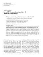
Figure 1: Baseline estimation based on the TP segment.
2. SCORE CALCULATION AND THEORETICAL
COMPUTATIONAL COMPLEXITY/MEMORY
OCCUPATION
The following results regarding computational complexity
are based on the estimation of the total number of opera-
tions. According to [28], operation involves any basic math-
ematical task performed by simple computational devices
(e.g., microprocessors), such as divison, sum, subtraction,
multiplication, and comparison (<, >, <

=, >=, ==,!=). In
this context, the computational complexity is abbreviated as
CC, and it is expressed in terms of n, the number of leads
used to perform ECG measurements.
The theoretical memory occupation (TMO) is defined as
the total number of variables that must be in memory in
order to perform all calculations leading to the score. This
total number is then multiplied by one byte, thus providing
the measurement of TMO in bytes.
2.1. Aldrich score [15]
In order to calculate the Aldrich score, the AMI must lead
to ST elevations higher than 0.1 mV, in at least two adjacent
leads, except for aVR. The isoelectric line is determined by
the TP segment (Figure 1), which is obtained by connecting
the first T point to the subsequent P point. Then the baseline
is traced as the horizontal line that passes through the
midpoint connecting the two preview ones, according to
Pmy
=
Ty− Py
2
,(1)
where Ty is the amplitude for the first T point [mV]; Py is
the amplitude for the subsequent P point [mV].
In the following, the AMI must be classified into anterior
or inferior. An anterior AMI leads to ST elevations in
leads DII, DIII, and aVF; whereas the inferior involves ST
elevations in V1–V4. If there are ST elevations in DI, aVL,
or V5-V6, the classification is also based on the leads cited
previously, but considering those with higher amplitude of

ST elevation.
If the AMI is anterior, the Aldrich score is calculated by
(2) as follows:
AS
ant
= 3·

1, 5·N
ST
− 0, 4

,(2)
where AS
ant
is the resulting Aldrich score and N
ST
is the
number of leads with ST elevation.
4 EURASIP Journal on Advances in Signal Processing
Table 1: T-wave morphology.
Type of T-wave Acronym
Necessary characteristics for the classification
T is the maximum peak of T-wave [mV]
High T-wave TT
{T ≥ 1.0mVinV2–V4} OR
{T ≥ 0.75 mV (7.5 mm) in V5} OR
{T ≥ 0.5 mV (5 mm) in DI or DII or aVF or V1 or V6}
OR
{T ≥ 0.25 mV (2.5 mm) in aVL or DIII}
Positive T-wave PT

{T ≥ 0.05 mV (0.5 mm)} anddonotfulfillTTcriteria
Flatten T-wave FT
T-wave with modulus
≤ 0.05 mV (0.5 mm)
T negative-terminating wave EN
{50% of initial positive T-wave ≥ 0.05 mV (0.5 mm)} and {the other part with
modulus
≥ 0.05 mV (0.5 mm)}.
Half-negative T-wave MN
{More than 50% of T-wave with negative modulus ≥ 0.05 mV (0.5mm)}
If the AMI is inferior, the ST elevation is measured in
millimeters at the J point, which may be considered the final
point of QRS complex, just before the ST, according to (3).
This measurement must be rounded to the next integer value:
Supra
ST
(d) =


Jy(d) − Pmy(d)


[mm], (3)
where d is the lead in which the ST elevation is estimated;
Jy(d) is the amplitude of the J point in lead d [mm]; Pmy is
the amplitude for the baseline, estimated by (1), which must
be converted into [mm].
Then the Aldrich score is calculated as follows:
AS
inf

= 3·

0.6·

Supra
ST
(II) + Supra
ST
(III)
+Supra
ST
(aVF)

+2

,
(4)
where AS
inf
is the Aldrich score and Supra
ST
(d)isestimated
by (3)atlead(d).
The result of the calculation, in any of the formulas (2)
or (4), is the percentage of myocardium under the risk of
necrosis as the AMI progresses.
The computational complexity (CC) and theoretical
memory occupation (TMO, n
= 12 leads) evaluations are
presented below.

(A) Baseline calculation for each lead, using (1):
CC
= 3n operations; TMO = 12 leads × 3variables=
36 variables.
(B) ST elevation estimation in 12 leads, using (3): TMO
= 12 leads × 2variables= 24 variables.
(C) Decision on AMI type (anterior or inferior)
(D) Estimation of Aldrich score, using (3)-(4)ifitis
inferior; or (2), if anterior.
(i) Inferior AMI: CC = 3n + 6 operations; TMO =
1variable.
(ii) Anterior AMI: 3n + 3 operations; TMO
= 2
variables.
Summing up all the operations described above, one
gets the final computational complexity (CC) and theoretical
memory occupation (TMO).
(i) Inferior AMI:
CC
Aldrich
= 6n + 6 operations; TMO
Aldrich
= 61 bytes.
(5a)
(ii) Anterior AMI:
CC
Aldrich
= 6n + 3 operations; TMO
Aldrich
= 62 bytes.

(5b)
For the most common case in clinical practice, n
= 12,
leading to CC
Aldrich
= 6 × 12 + 6 = 78 operations.
2.2. Selvester score [13, 25]
Three steps are necessary in order to estimate the Selvester
score, according to the table presented in Ta bl e 6 which
describes the rules of this procedure.
Step (i): the score is intialized with zero.
Step (ii); the leads are analyzed, observing the group of
rules in Selvester table (see Ta bl e 6).
This step involves the knowledge of the maximum peaks
associated with Q, R,andS,aswellasthedurationofQ-
wave and R-wave. From Selvester table, within one single
lead, there are one or more rules, which are divided into
groups (a) and (b). For each group, the rules must be checked
upside down (from the top to the bottom), until one rule is
evaluated as “true.” Once the “true rule” is identified for the
group, its points are summed to compose the overall score.
For instance, considering lead I, if the first rule of group
(b) (Ramp <
= Qamp) is satisfied, one must add 1 point to
the score.
Step (iii): after all rules are evaluated, following the order
of leads established by the Selvester table, the points must be
summed up, leading to the final Selvester score.
In terms of computational complexity, the Selvester score
uses basically sums and comparisons. Based on Ta bl e 6 ,for

the worst case, there are 53 comparisons and 21 sums,
J. B. Destro-Filho et al. 5
Table 2: Pathological Q-wave classification conditions.
LEAD
CONDITION (Qdur is the duration of Q wave
[millisecond])
DI
Qdur
≥ 30 ms (0.75 mm)
DII
Qdur
≥ 30 ms (0.75 mm)
DIII
Qdur
≥ 30 ms (0.75 mm) in aVF
aVL
Qdur
≥ 30 ms (0.75 mm)
aVF
Qdur
≥ 30 ms (0.75 mm)
V1
Any Qdur
V2
Any Qdur
V3
Any Qdur
V4
Qdur
≥ 20 ms (0.5 mm)

V5
Qdur
≥ 30 ms (0.75 mm)
V6
Qdur
≥ 30 ms (0.75 mm)
leading to 74 operations for the 12-lead ECG. In terms of
TMO, for each lead, one should estimate amplitude and
duration for Q, R,andS waves, thus leading to 12 leads
× 6variables= 72 variables. One should also consider 11
composite quantities such as Q/R, from the Selvester table.
In consequence, one should write the CC and the TMO as
follows:
CC
Selvester
= 74 operations;
TMO
Selvester
= 83 bytes; (n = 12 leads).
(6)
2.3. Anderson-Wilkins score [19]
The Anderson-Wilkins acuteness score is based on the simul-
taneous analysis and classification of ST elevation, the T-
wave variations, and the presence/absence of pathological Q
waves. Tab le 1 shows T-wave classification, whereas Tab le 2
explains the conditions, established particularly at each ECG
lead, for Q-wave being considered pathological.
The calculation of Anderson-Wilkins score employs the
following steps.
Step 1. Diagnose AMI with ST elevation, which must be

greater than 0.1 mV and must take place at least in two
adjacent leads, except in aVR, considering TP segment as
baseline and measurements with respect to J point.
Step 2. For each lead, classify the T-waves according to
Ta bl e 1 as
{TT,PT,FT,EN,MN}.
Step 3. For each lead, considering Ta b le 2 , establish whether
pathological Q-waves take place.
Step 4. Classify the leads into classes according to Tab le 3.For
one lead being considered of one specific class, it must satisfy
the three conditions (ST elevation, T-wave classification, and
pathological Q presence) at the same time.
Step 5. Calculate the Anderson-Wilkins score using (7):
EAW
=
4·nD
1A
+3·nD
1B
+2·nD
2A
+ nD
2B
nD
1A
+ nD
1B
+ nD
2A
+ nD

2B
,(7)
where nD
1A
is the number of leads pertaining to class 1A;
nD
1B
is the number of leads classified as 1B; nD
2A
is the
number of 2A leads, and nD
2B
is the number of 2B leads.
In consequence, the Anderson-Wilkins score is estimated
with amplitude between 0–4, for which the high values are
associated with more acute ischemia.
Based on Steps 1–5 described above, there are 18n +37
operations required to estimate the Anderson-Wilikins score,
and considering the 12-lead ECG, there are 253 operations in
the worst case scenario. Thus CC is expressed as below:
CC
A-Wilkins
= 18n +37operations. (8a)
In terms of TMO, one should analyze the algorithm step
by step, considering the worst case scenario presented below.
Step 1. Estimate baseline by (1) and the ST elevation based
on (3)foralln
= 12 leads.
3
× 12 + 1 × 12 = 48 variables.

Step 2. Classification of T-waves according to Tab le 1.
13 variables (including all T amplitudes of all leads) + all
12 classifications
= 25 variables.
Step 3. Classification of Q-waves according to Tab le 2 .
11 variables (including all Q durations of all leads) + all
12 classifications
= 23 variables.
Step 4. Finding a class for all leads according to Ta bl e 3.
For T-wave classification column, there are 2
× 12 = 24
variables for comparisons.
For Pathological Q waves, there are 12 variables for
comparisons.
Step 5. Final calculation of the score based on (7).
There are 9 variables, including the score itself.
Summing up all the TMO results presented in the last
paragraph:
TMO
A-Wilkins
= 141 bytes (n = 12 leads). (8b)
3. METHODS
Based on the procedures described in Section 2, the three
scores were implemented as algorithms on a C++ platform.
The Microsoft Foundation Classes (MFCs) library was
employed for the graphical user interface, as well as for the
use of a library, devoted to the assessment of processing
time. All simulations were carried out using an IBM-PC
microcomputer with the following characteristics. Processor:
AMD Semprom 2400 + 1.668 GHz; Motherboard: ASUS

A7V8X-X; RAM memory: 768 MB DDR, 333 MHz; HD
memory: 120 GB.
The input to these computer programs is a matrix
containing ECG data necessary for all calculations, which
involves measurements taken at P-wave, the QRS complex, J
point, and T-wave. There are twelve lines in the matrix, each
one associated with one specific lead. The vector C, defining
each line of this matrix, is described below:
C
=

C1 C2

,(9a)
where C1 and C2 are subvectors, respectively, associated with
the first complete ECG cycle and the subsequent complete
6 EURASIP Journal on Advances in Signal Processing
Table 3: Grouping leads into classes for Anderson-Wilkins score calculation.
Class of lead (acronym)
ST elevation + indicates
presence,
− indicates absence
T-wave classification (see
acronyms in Ta bl e 1 )
Pathological Q-waves (Tab le 2) + indicates
presence, − indicates absence
1A
+or
− TT −
1B

+PT
−
2A
+or
− TT +
2B
+PT +
3
+EMorFT +
4
+MN +
U
+EM,FT,orMN
−
ECG cycle, as defined below:
C1
= [Pix,Piy,Pmx, Pmy, Pfx, Pfy, Qix, Qiy, Qmx,
Qmy, Qfx, Qfy, Rix, Riy, Rmx, Rmy, Rfx,Rf y,
Jmx,Jmy, Six,Siy, Smx, Smy, Sfx, Smy,
{Tix, Tiy, , Tmx, Tmy, , Tfx, Tfy}],
(9b)
where i stands for initial, m for maximum, f for final, x
for time [millisecond], and y for amplitude [mV]. Notice
that the subset
{Ti, , Tm, , Tf} is composed of all the
samples of T-wave. Considering that the ECG signal is
sampled at one millisecond, that the normal T-wave lasts
about 120 milliseconds [29], and also considering all the
elements of the vector in (9b), the length of vector C in (9a)
is 2

× (26 +2 × 120) = 532 elements. Subvector C2 is defined
in a similar way as in (9b), including the same data described
in this paragraph, however, the P, Q, R, J, S and T quantities
are associated to the subsequent ECG cycle, with respect to
that one leading to the definition of subvector C1.
For Aldrich score calculation, just the data from points
{P, Q, R, J, S, T, P2(secondP)} are necessary. The Selvester
score uses waves and not only specific peak points of the
ECG waves, thus requiring amplitude and time for initial,
maximum, and ending points of the P, Q, R, S, T waves. For
Anderson-Wilkins score, the input must include initial and
final Q-wave point data, as well as all the samples associated
with the T-wave.
It is supposed that automatic recognition of the elements
in each vector (9a)-(9b) is perfect, so that the computer has
already analyzed the raw digital ECG data and generated
the input data matrix, the lines of which are given by
(9a)-(9b), for all leads. In consequence, our computational
evaluation does not take into consideration time processing
and memory occupation associated with the identification of
any sample in (9a)-(9b).
Processing time is estimated based on the m
Timer .
Start(1,0) routine, which starts the winmm.dll timer. Multi-
media timers allow the best resolution for event firing, which
is a necessary feature to accomplish the task of processing-
time evaluation.
In order to measure memory occupation of the algo-
rithms, the Windows XP Task Manager was used. This
operational system routine enables the assessment of mem-

ory occupation of any process, by monitoring the Task
Manager application. For instance, suppose that one needs
to measure the memory occupation for the Notepad process.
The graphical user interface of Tas k M an a ge r displays status
and memory occupation of the process list, thus the Notepad
process data can be monitored during runtime.
In order to avoid interference of other softwares or
processes on the measurements, just the windows associated
with the C++ compiler, Multimedia Timer, and the Ta sk
Manager remained open during simulations.
For each score algorithm, we have carried out a Monte
Carlo simulation study of both memory occupation (MO)
and time processing (TP), by estimating the average MO in
Kilobytes and the average TP in milliseconds. Results to be
presented in Section 4 suppose averages based on one million
(1000000) different experiments. The input matrices for all
these evaluations, containing digitized ECG data, were the
same for all the three algorithms. The one million different
input matrices were randomly generated based on average
values reported in the literature [13, 15, 19, 26, 29], to which
slow-amplitude random numbers were added by software
processing. The “slow-amplitude” adjectif means that, for
voltages, amplitudes do not exceed 1 millivot; whereas for
times, amplitudes do not exceed 10 milliseconds.
4. RESULTS
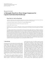
Figure 2 depicts the graphic representation of (5a)-(5b),
(8a)-(8b), and (6). In order to generate this figure, we have
considered clinical practical values [29] for the number of
leads n, so that n
={2,3, 6, 12,14,16, 20, 50}. Notice that

n
= 2, 3 refers to simple cardiac monitoring; n = 12 is the
standard ECG configuration; n
= 14, 16 may be carried out
in order to get specific information from any cardiac region;
whereas n
= 50 is associated with mapping the epicardial
surface.
Ta bl e 4 presents CC and TMO for the daily situation
n
= 12 leads, as well as its product CC × TMO, which
characterizes the global algorithm complexity considering,
at the same time, memory occupation and the number of
operations. These values were obtained at (5a)-(5b), (8a)-
(8b), and (6).
In Figure 2, notice that computational complexity is
evaluated in terms of the global number of operations
necessary for performing one calculation of the scores.
Results are very close to each other, but Aldrich score presents
J. B. Destro-Filho et al. 7
Table 4: Theoretical computational complexity (CC) and memory occupation (TMO); n = 12.
Score Theoretical CC [operations] Theoretical memory occupation [bytes] CC × TMO [operations · bytes]
Aldrich 78 62 4836
Selvester 74 83 6142
Anderson-Wilkins 253 141 35673
Table 5: Average experimental results for each score, considering Figure 3 (n = 12).
Score
Processing time (PT) [millisecond] Memory occupation (MO) [Kbytes]
ProductofaveragePT
× average MO

[millisecond
× Kbytes]
Average Standard deviation Average Standard deviation
Anderson-Wilkins
0.8845 0.0209 154.22 7.7323 136.41
Selvester
0.7152 0.0038 149.30 11.3534 106.80
Aldrich
0.4485 0.2864 111.70 20.1108 50.10
the lowest complexity as the number of leads n grows. Ta bl e 4
points out clearly that Aldrich score is the less complex one
for n
= 12, whereas Anderson-Wilkins is the most complex.
This last score, from the theoretical viewpoint, requires too
much operations and bytes per iteration, with respect to the
other two scores.
Figure 3 presents experimental results relating memory
occupation and execution time for n
= 12, which is the most
common clinical situation.
From Figure 3, one may state that the memory occupa-
tions of the three algorithms are very similar to each other.
Notice also that, holding a value of memory occupation
fixed, Selvester score PT is lower than Anderson-Wilkins PT.
In addition, whereas for Selvester score and for Anderson-
Wilkins score the MO does not change too much for all the
ranges of PT, the memory occupation for Aldrich score does
vary as a function of PT. In consequence, the Selvester score is
the most stable implementation, since its plot (see Figure 3)
is a straight line, which may be associated to little variance in

terms of the quantity MO. On the other hand, Aldrich score
is quite unstable.
Ta bl e 5 depicts average results that can be estimated
based on Figure 3, also supposing n
= 12.
Ta bl e 5 confirms previous conclusions discussed in the
last paragraphs. The unstability of Aldrich score is clearly
depicted by the highest values attained by its variance, both
in terms of PT and of MO. Selvester score, on the other
hand, is the most stable algorithm. Aldrich score, however,
presents the lowest average PT and the lowest average MO.
In addition, if one compares the last column of Ta bl e 5
(experimental product PT
× MO) to the last column of
Ta bl e 4 (theoretical product CC
× TMO), simulation and
theory agree quite well with each other, and both put forward
that Aldrich score is the least complex algorithm.
5. CONCLUSIONS AND FUTURE WORK
Results point out that performances of algorithms are very
close to each other, either as the number of leads n grows
(Figure 2), or in the daily situation of n
= 12 (Figure 3,
Ta bl es 4 and 5). However, as n varies, Aldrich score presents
the lowest theoretical computational complexity. For n
=
0
200
400
600

800
1000
Number of operations
10 20 30 40 50
Number of leads (n)
Selvester
Anderson-Wilkins
Aldrich
Aldrich score
Selvester score
Anderson-Wilkins score
Figure 2: Theoretical computational complexity of (5a)-(5b), (8a)-
(8b), and (6); depicted as a function of n
={2, 3, 6, 12, 14, 16,
20, 50
}.
100
120
140
160
180
Memory occupation
(Kbytes)
00.10.20.30.40.50.60.70.80.9
Average-total processing time (ms)
Selvester
Anderson-Wilkins
Aldrich
Anderson-Wilkins score
Selvester score

Aldrich score
Figure 3: Experimental processing time (PT) versus memory
occupation (MO) for n
= 12 leads.
12, Aldrich score seems to be the most efficient one, since
it presents the lowest average memory occupation and the
lowest average processing time. This conclusion was achieved
from both theory and experiments. However, as one also
considers the case n
= 12, the standard deviations of
both Selvester and Anderson-Wilkins scores are very little in
comparison with those associated with Aldrich score, thus
pointing out that the last algorithm is quite unstable.
8 EURASIP Journal on Advances in Signal Processing
Table 6: Rules for Selvester score estimation [13].
Rule ECG lead Criteria Points Maximum points/lead
1
I
(a) Qdur >= 30 ms 1
2
2
(b)
Ramp <
= Qamp 1
3 Ramp <
= 0.2 mV 1
4
II (a)
Qdur >= 40 ms 2
2

5 Qdur >
= 30 ms 1
6
aVL
(a) Qdur >= 30 ms 1
2
7(b)Ramp <
= Qamp 1
8
aVF
(a)
Qdur >= 50 ms 3
5
9 Qdur >
= 40 ms 2
10 Qdur >
= 30 ms 1
11
(b)
Ramp <
= Qamp 2
12 Ramp <
= 2∗Qamp 1
13 V1 anterior (a) Any Q 11
14
V1 posterior
(a) Ramp >= Samp 1
4
15
(b)

Rdur >
= 50 ms 2
16 Ramp >
= 1mV 2
17 Rdur >
= 40 ms 1
18 Ramp >
= 0.6 mV 1
19 (c) Qamp AND Samp <
= 0.3 mV 1
20
V2 anterior (a)
Any Q 1
1
21 Rdur <
= 10 ms 1
22 Ramp <
= 0.1 mV 1
23 Ramp <
= Ramp(V1) 1
24
V2 posterior
(a) Ramp >= 1.5∗Samp 1
4
25
(b)
Rdur >
= 60 ms 2
26 Ramp >
= 2mV 2

27 Rdur >
= 50 ms 1
28 Ramp >
= 1.5 mV 1
29 Qamp AND Samp <
= 0.4 mV 1
30
V3 (a)
Any Q 1
1
31 Rdur <
= 20 ms 1
32 Ramp <
= 0.2 mV 1
33
V4
(a) Qdur >= 20 ms 1
3
34
(b)
Ramp <
= 0.5∗Samp 2
35 Ramp <
= 0.5∗Qamp 2
36 Ramp <
= Samp 1
37 Ramp <
= Qamp 1
38 Ramp <
= 0.7 mV 1

39
V5
(a) Qdur >= 30 ms 1
3
40
(b)
Ramp <
= Samp 2
41 Ramp <
= Qamp 2
42 Ramp <
= 2∗Samp 1
43 Ramp <
= 2∗Qamp 1
44 Ramp <
= 0.7 mV 1
J. B. Destro-Filho et al. 9
Table 6: Continued.
Rule ECG lead Criteria Points Maximum points/lead
45
V6
(a) Qdur >= 30 ms 1
3
46
(b)
Ramp <
= Samp 2
47 Ramp <
= Qamp 2
48 Ramp <

= 3∗Samp 1
49 Ramp <
= 3∗Qamp 1
50 Ramp <
= 0.6 mV 1
Where, Qdur, Rdur: duration of, respectively, Q-wave and of R-wave [millisecond]. Qamp, Ramp: maximum peak of, respectively, Q-wave and of R-wave
[mV]. Samp: maximum peak of S-wave [mV].
Average processing times and average memory occupa-
tions of Ta b le 5 must be carefully considered. In fact, they
point out that simple computer platforms based on C++
do enable fast estimation of AMI scores without too much
memory requirements. Particularly, average processing times
should be compared to the times required by manual
measurements commonly performed by medicines. In our
research group, medical science undergraduate students with
good clinical practice take about fifteen minutes in average
for estimating the simple Aldrich score.
Future work involves the assessment of both memory
occupation and time processing as the number of leads
n varies. The computational complexity of Selvester score
should also be calculated as a function of n, and the unsta-
bility of Aldrich score should be better evaluated. We are also
developing a more accurate methodology for assessing MO
and TP, based on well-established C++ functions that can
be inserted into the algorithm implementation. Finally, the
automatic estimation of P, Q, R, S, J and T quantities from
digital ECG recordings is on course, so that to include this
computational effort in our evaluation.
ACKNOWLEDGMENTS
The authors would like to thank undergraduate medical

science students Geraldo RR Freitas and Lucila SS Rocha, as
well as Professor Elmiro S Resende (Medical Sciences School,
UFU), for their technical contribution regarding bibliogra-
phy, as well as for details on the procedure for estimating the
AMI scores. They are also indebted to Professor G. S. Wagner,
from Duke University Medical Center, USA, for his regular
technical disscussions and support to their research.
REFERENCES
[1] DATASUS, “Health Information and Biostatistical Index,”
Official website of the Brazilian National Health Minis-
try, November 2007, />.php.
[2] R. F. Gillum, “Trends in acute myocardial infarction and
coronary heart disease death in the United States,” Journal of
the American College of Cardiology, vol. 23, no. 6, pp. 1273–
1277, 1994.
[3] The Joint European Society of Cardiology/American College
of Cardiology, “Myocardial infarction redefined—a consensus
document,” European Heart Journal, vol. 21, no. 18, pp. 1502–
1513, 2000.
[4] S.A.Achar,S.Kundu,andW.A.Norcross,“Diagnosisofacute
coronary syndrome,” American Family Physician,vol.72,no.1,
pp. 119–126, 2005.
[5]D.Brieger,K.A.Eagle,S.G.Goodman,etal.,“Acute
coronary syndromes without chest pain, an underdiagnosed
and undertreated high-risk group: insights from the global
registry of acute coronary events,” Chest, vol. 126, no. 2, pp.
461–469, 2004.
[6] S. A. Hahn and C. Chandler, “Diagnosis and management
of ST elevation myocardial infarction: a review of the recent
literature and practice guidelines,” The Mount Sinai Journal of

Medicine, vol. 73, no. 1, pp. 469–481, 2006.
[7] H. Blanke, M. Cohen, G. U. Schlueter, K. R. Karsch, and K. P.
Rentrop, “Electrocardiographic and coronary arteriographic
correlations during acute myocardial infarction,” The Ameri-
can Journal of Cardiology, vol. 54, no. 3, pp. 249–255, 1984.
[8] P. Schweitzer, “The electrocardiographic diagnosis of acute
myocardial infarction in the thrombolytic era,” American
Heart Journal, vol. 119, no. 3, part 1, pp. 642–654, 1990.
[9] J. E. Madias, “Use of precordial ST-segment mapping,”
American Heart Journal, vol. 95, no. 1, pp. 96–101, 1978.
[10] B. L. Nielsen, “ST-segment elevation in acute myocardial
infarction: prognostic importance,” Circulation, vol. 48, no. 2,
pp. 338–345, 1973.
[11] R. Sch
¨
oder, K. Wegscheider, K. Schr
¨
oder, R. Dissmann, and
W. Meyer-Sabellek, “Extent of early ST segment elevation
resolution: a strong predictor of outcome in patients with
acute myocardial infarction and a sensitive measure to com-
pare thrombolytic regimens. A substudy of the International
Joint Efficacy Comparison of Thrombolytics (INJECT) trial,”
Journal of the American College of Cardiology,vol.26,no.7,pp.
1657–1664, 1995.
[12] Y. Birnbaum and D. L. Ware, “Electrocardiogram of acute ST-
elevation myocardial infarction: the significance of the various
“scores”,” Journal of Electrocardiology, vol. 38, no. 2, pp. 113–
118, 2005.
[13] R. H. Selvester, R. E. Sanmarco, J. C. Solomon, and G. S.

Wag ner, “ Th e E CG : Q RS c han ge,” in Myocardial Infarction:
Measurement and Intervention,G.S.Wagner,Ed.,Develop-
ments in Cardiovascular Medicine, chapter 14, pp. 23–50,
Martinus Nijhoff, The Hague, The Netherlands, 1982.
[14] G. S. Wagner, C. J. Freye, S. T. Palmeri, et al., “Evaluation of
a QRS scoring system for estimating myocardial infarct size. I.
Specificity and observer agreement,” Circulation, vol. 65, no. 2,
pp. 342–347, 1982.
[15] H. R. Aldrich, N. B. Wagner, J. Boswick, et al., “Use of
initial ST-segment deviation for prediction of final electro-
cardiographic size of acute myocardial infarcts,” The American
Journal of Cardiology, vol. 61, no. 10, pp. 749–753, 1988.
10 EURASIP Journal on Advances in Signal Processing
[16] P. Clemmensen, P. Grande, H. R. Aldrich, and G. S. Wagner,
“Evaluation of formulas for estimating the final size of acute
myocardial infarcts from quantitative ST-segment elevation
on the initial standard 12-lead ECG,” Journal of Electrocardi-
ology, vol. 24, no. 1, pp. 77–80, 1991.
[17] M. L. Wilkins, C. Maynard, B. H. Annex, et al., “Admission
prediction of expected final myocardial infarct size using
weighted ST-segment, Q wave, and T wave measurements,”
Journal of Elect rocardiology, vol. 30, no. 1, pp. 1–7, 1997.
[18] B. Hed
´
en, R. Ripa, E. Persson, et al., “A modified Anderson-
Wilkins electrocardiographic acuteness score for anterior or
inferior myocardial infarction,” American Heart Journal, vol.
146, no. 5, pp. 797–803, 2003.
[19]M.L.Wilkins,A.D.Pryor,C.Maynard,etal.,“Anelectro-
cardiographic acuteness score for quantifying the timing of a

myocardial infarction to guide decisions regarding reperfusion
therapy,” The American Journal of Cardiology, vol. 75, no. 8, pp.
617–620, 1995.
[20] R. S. Ripa, E. Persson, B. Hed
´
en, et al., “Comparison between
human and automated electrocardiographic waveform mea-
surements for calculating the Anderson-Wilkins acuteness
score in patients with acute myocardial infarction,” Journal of
Electrocardiology, vol. 38, no. 2, pp. 96–99, 2005.
[21] K. E. Corey, C. Maynard, O. Pahlm, et al., “Combined
historical and electrocardiographic timing of acute anterior
and inferior myocardial infarcts for prediction of reperfusion
achievable size limitation,” The American Journal of Cardiol-
ogy, vol. 83, no. 6, pp. 826–831, 1999.
[22] L. S
¨
ornmo and P. Laguna, Bioelectrical Signal Processing
in Cardiac and Neurological Applications, Academic Press,
Amsterdam, The Netherlands, 1st edition, 2005.
[23] M. J. Eskola, K. C. Nikus, L M. Voipio-Pulkki, et al., “Com-
parative accuracy of manual versus computerized electrocar-
diographic measurement of J-, ST- and T-wave deviations in
patients with acute coronary syndrome,” The American Journal
of Car diology, vol. 96, no. 11, pp. 1584–1588, 2005.
[24] M.M.Pelter,M.G.Adams,andB.J.Drew,“Computerversus
manual measurement of ST-segment deviation,” Journal of
Electrocardiology, vol. 30, no. 2, pp. 151–156, 1997.
[25] B. M. Hor
´

a
ˇ
cek,J.W.Warren,A.Albano,etal.,“Development
of an automated Selvester Scoring System for estimating the
size of myocardial infarction from the electrocardiogram,”
Journal of Elect rocardiology, vol. 39, no. 2, pp. 162–168, 2006.
[26] F. Badilini, T. Erdem, W. Zareba, and A. J. Moss, “ECGScan:
a method for conversion of paper electrocardiographic print-
outs to digital electrocardiographic files,” Journal of Electrocar-
diology, vol. 38, no. 4, pp. 310–318, 2005.
[27] C. Ho, B. Eloff, F. Lacy, L. Shoemaker, and E. Mallis, “Issues
for ECG devices with preinstalled leads and reduced leads,”
Journal of Electrocardiology,vol.39,no.4,supplement1,p.
S33, 2006.
[28] H. S. Wilf, Algorithms and Complexity, AK Peters, London,
UK, 2002.
[29] J. G. Webster, Ed., Medical Instrumentation: Application and
Design, John Wiley & Sons, New York, NY, USA, 3rd edition,
1998.