Báo cáo hóa học: " Research Article Extraction of Desired Signal Based on AR Model with Its Application to Atrial Activity " doc

Hindawi Publishing Corporation
EURASIP Journal on Advances in Signal Processing
Volume 2008, Article ID 728409, 9 pages
doi:10.1155/2008/728409
Research Article
Extraction of Desired Signal Based on AR Model with Its
Application to Atrial Activity Estimation in Atrial Fibrillation
Gang Wang,
1, 2
Ni-ni Rao,
1
Simon J. Shepherd,
2
and Clive B. Beggs
2
1
School of life Science and Technology, University of Electronic Science and Technology of China, Chengdu 610054, China
2
Medical Biophysics Group, School of Engineer ing, Design and Technology, University of Bradford, BD7 1DP Bradford, UK
Correspondence should be addressed to Ni-ni Rao,
Received 28 July 2007; Revised 15 February 2008; Accepted 23 April 2008
Recommended by An
´
ıbal Figueiras-Vidal
The use of electrocardiograms (ECGs) to diagnose and analyse atrial fibrillation (AF) has received much attention recently. When
studying AF, it is important to isolate the atrial activity (AA) component of the ECG plot. We present a new autoregressive (AR)
model for semiblind source extraction of the AA signal. Previous researchers showed that one could extract a signal with the
smallest normalized mean square prediction error (MSPE) as the first output from linear mixtures by minimizing the MSPE.
However the extracted signal will be not always the desired one even if the AR model parameters of one source signal are known.
We introduce a new cost function, which caters for the specific AR model parameters, to extract the desired source. Through
theoretical analysis and simulation we demonstrate that this algorithm can extract any desired signal from mixtures provided that

its AR parameters are first obtained. We use this approach to extract the AA signal from 12-lead surface ECG signals for hearts
undergoing AF. In our methodology we roughly estimated the AR parameters from the fibrillatory wave segment in the V1 lead,
and then used this algorithm to extract the AA signal. We validate our approach using real-world ECG data.
Copyright © 2008 Gang Wang et al. This is an open access article distributed under the Creative Commons Attribution License,
which permits unrestricted use, distribution, and reproduction in any medium, provided the original work is properly cited.
1. INTRODUCTION
In recent years, there has been considerable interest in
the electrical and physiological mechanisms associated with
atrial fibrillation (AF) [1–4]. AF is a relatively common
arrhythmia, which occurs when the atria depolarize repeat-
edly in an irregular uncontrolled manner. During AF,
electrical discharges come from other parts of the atria,
rather than solely from the sinoatrial (SA) node. These
abnormal irregular discharges are very rapid and result
in ineffective contraction of the atria, so that they quiver
rather than beat as a unit. This reduces the ability of the
atria to discharge blood into the ventricles, thus impairing
the performance of the heart. AF is of clinical importance
because it is associated with an increased risk of morbidity
and mortality, particularly amongst the elderly who are more
prone to this condition.
AF is generally diagnosed by visual inspection of the
surface electrocardiogram (ECG). On an ECG plot, AF is
characterized by a plot which has no clear P-wave, only a fine
apparently disorganized oscillation (known as a fibrillatory
or F-wave), and a ventricular response which is fast and
irregular. When studying AF it is important to isolate the
atrial activity (AA) component of the ECG plot. However,
because the electrical activity of the ventricles is of greater
amplitude of the atria, it is difficult to identify the atrial

component. Several methods have been developed to address
this problem. Some are based on average beat subtraction
(ABS), which assumes that the AA is uncoupled with the
ventricular activity (VA). This approach uses an average of
the ventricular QRST complexes which is then subtracted
from the wave to determine AA [5]. However, this approach
is limited by the small number of VA average templates
available for general VA approximation [3]. Recently, meth-
ods which utilize blind source separation (BSS) have been
developed for extracting AA signals from ECG plots [6–10].
The objective of this approach is to recover the unknown
source signal from the mixture without knowing the mixing
channels. While BSS appears promising, it has the drawback
that it requires considerable computational power. In an
attempt to address this issue, we undertook a study using a
blind source extraction (BSE) approach to solve the problem.
BSE is a powerful technique related to BSS [11, 12], which
has become one of the major research areas in signal
2 EURASIP Journal on Advances in Signal Processing
processing. The approach taken in BSE is to sequentially
extract small subsets from the source signal, which are
independent from each other, but linearly combined in the
observations. Compared with BSS, BSE requires a much
lower computational load and is therefore less expensive. As a
result it has received considerable interest and has been used
in various fields such as biomedical signal processing [13]
and speech processing [11, 12].
Many algorithms designed for BSE have been proposed,
including those employing high-order statistics (HOS) [14,
15] and those employing second-order statistics (SOS) [13,

15–19]. Cichocki and Amari [11] give a comprehensive
overview of these algorithms. However, these algorithms are
generally designed to extract signals in a specific order [19],
or extract special signals, such as fetal ECG [13] and fMRI
data [14], and they do not always work well when dealing
with an AA signal. AA sources have a main peak between
3.5–10 Hz [10], where the observed ECG plot has two or
more apparently random peaks. So it is not possible to
estimate directly distinct periods in the signal. Consequently,
algorithms based on periodic structure [13, 16, 17, 19]will
fail. Moreover, the AA wave is not stationary, so it is difficult
for a constrained independent component analysis (ICA)
algorithm [14] to select the referent signal and thus extract
the AA data.
Given that AA signals exhibit a narrowband spectrum
[20, 21] with main frequencies between 3.5–10 Hz [8],
in our study we came to the conclusion that the linear
predictor or autoregressive (AR) model could be regarded
as stable. Moreover, we determined that it was possible
to estimate the AR parameters from the fibrillatory wave
segment of the surface ECG plot. While BSE algorithms
[17, 19] employing a linear predictor usually minimize the
normalized mean square prediction error (MSPE), they may
not extract the specific signal, even though its AR parameters
may be known. In this paper, we therefore introduced a
new cost function, which caters for the specific AR model
parameters, and propose an algorithm based on eigenvalue
decomposition (EVD) to extract the desired signal. In the
paper, we validate this algorithm and illustrate how it can be
used to estimate the AR parameters of the AA wave signal.

We also summarize techniques that can be used to extract
AA signals based on a BSE approach.
2. LIMITATION OF MSPE
In BSE, we observe an m-dimensional stochastic signal
vector x that is regarded as the linear mixture of an m-
dimensional zero-mean and unit-variance vector s, that is,
x
= As,whereA is an unknown mixing matrix. The goal of
BSE is to find a demixing vector w such that y
= w
T
x =
w
T
As is an estimated source signal up to a scalar. To make
algorithm more robust and faster, prewhitening is often used
to transform the observed signals x to x
= Vx, such that
E
{xx
T
}=VA E{ss
T
}A
T
V
T
= VA A
T
V

T
= I,whereV is
a prewhitening matrix. Therefore, for convenience, in this
paper we will assume that x has been prewhitened in the
following, that is, E
{xx
T
}=I, A is an orthogonal matrix,
and w
T
w = 1.
If we assume that the sources are not correlated with
each other and have different temporal structures, then the
following relations are satisfied:
E

s
i
(n)s
j
(n −τ)

=
0, ∀i
/
= j,0≤ τ ≤ p,(1)
where p is the length of the linear predictor or AR model.
Then the instantaneous prediction error (PE) denoted by
e(n)isasfollows:
e(n)

= y(n) −b
T
Y(n),
b =

b
1
, b
2
, , b
P

T
,
Y(n) =

y(n −1), y(n − 2), , y(n − p)

T
,
y(n)
= w
T
x(n),
x(n) =

x
1
(n), x
2

(n), , x
m
(n)

T
,
(2)
where b is the AR parameters of a desired signal.
It has been shown by Liu et al. [17, 19] that source
signals can be extracted successfully by minimizing the
normalized MSPE E
{e
2
(n)} as long as they have different
temporal structures. The corresponding cost function is
the normalized MSPE E
{e
2
(n)}/E{y
2
(n)}.Asmentioned
above, we assume here that x has been prewhitened
and thus that the output power of the demixing vector
E
{y
2
(n)} is unity. Therefore, the cost function can be set as
E
{e
2

(n)}.
If we know the AR model of the desired source sig-
nal, s
1
(n), then we can easily identify its linear predictor
coefficients. The PE of the extracted signal therefore can be
written as
e(n)
= y(n) −b
T
Y(n)
= w
T
x(n) −

b
1
, b
2
, , b
P

×

w
T
x(n −1),w
T
x(n −2), ,w
T

x(n − p)

T
= w
T
x(n) −w
T
p

i=1
b
i
x(n −i)
= w
T

x(n) −
p

i=1
b
i
x(n −i)

.
(3)
Denote
z(n)
=


x(n) −
p

i=1
b
i
x(n −i)

. (4)
The normalized MSPE is
E

e
2
(n)

E

y
2
(n)

=
E

w
T
z(n)z
T
(n)w


E

w
T
x(n)x
T
(n)w

=
w
T
E

z(n)z
T
(n)

w
w
T
w
.
(5)
Gang Wang et al. 3
Moreover,
E

z(n)z
T

(n)

=
E

x(n) −
p

i=1
b
i
x(n −i)

x(n) −
p

i=1
b
i
x(n −i)

T

=
E

As(n)−
p

i=1

b
i
As(n −i)

As(n)−
p

i=1
b
i
As(n −i)

T

=
AE

s(n) −
p

i=1
b
i
s(n −i)

s(n) −
p

i=1
b

i
s(n −i)

T

A
T
.
(6)
Denote
R
p
= E

s(n) −
p

i=1
b
i
s(n −i)

s(n) −
p

i=1
b
i
s(n −i)


T

(7)
which is a diagonal matrix with the help of expres-
sion (1), and whose diagonal element R
p
(j, j) equals the
MSPEE
{{e
2
j
(n)}} of the corresponding source signal:
R
p
(j, j) = E

e
2
j
(n)

=
E

s
j
(n) −b
T
S
j

(n)

2

, j = 1,2, , m.
S
j
(n) =

s
j
(n −1),s
j
(n −2), , s
j
(n − p)

T
.
(8)
Then the normalized MSPE becomes
E
{e
2
(n)}
E{y
2
(n)}
=
w

T
AR
p
A
T
w
w
T
w
(9)
which implies that the minimization of the normalized
MSPE under the constraint w
T
w = 1 is equivalent to finding
the eigenvector corresponding to the minimal eigenvalue of
the real symmetric matrix E
{z(n)z
T
(n)}. Moreover, since A
is orthogonal and R
p
is diagonal matrix, theoretically the
minimal eigenvalue is equivalent to the minimum of the
diagonal elements R
p
(j, j)(j = 1, 2, , m). Thus we can
conclude that the first extracted signal by this method is the
one whose MSPE is minimal for a given AR parameter.
However,thisargumentmaynotbeasstraightforward
as it seems, because it raises interesting questions as to

whether or not the desired source signal has the minimum
normalized MSPE among its sources. If, for example, we
consider the benchmarks s
1
, s
2
, s
3
,ands
4
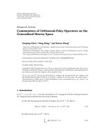
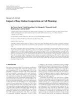
utilized in [19],
which are shown in Figure 1 (which can be found in the file
Abio7.mat provided in the ICALAB toolbox with book [11]),
it is possible to calculate using (8) the MSPEs of the four
signals for the given AR parameter of the different sources.
The results of this analysis are summarized in Ta ble 1 for
p
= 10 and in Ta ble 2 for p = 20, where the minimum
data in each row are accented with bold cases. In Ta ble 1 we
can see that s
3
, s
4
, s
4
,ands
4
exhibit a minimum normalized
MSPE separately for the given AR parameters of s
1

, s
2
, s
3
,
and s
4
,asdos
3
, s
4
, s
3
,ands
4
in Ta ble 2. In other words,
500040003000200010000
500040003000200010000
500040003000200010000
500040003000200010000
−5
0
5
s
4
−10
0
10
s
3

−5
0
5
s
2
−5
0
5
s
1
Figure 1: Four source signals in simulations.
Table 1: The MSPE of different sources for a different given AR
parameter (p
= 10).
MSPE of s
1
MSPE of s
2
MSPE of s
3
MSPE of s
4
Given AR of s
1
0.9974 0.9559 0.9459 0.9596
Given AR of s
2
1.9918 0.5176 0.2581 0.1937
Given AR of s
3

48.5098 4.8560 0.0731 0.0309
Given AR of s
4
4.0648 0.9520 0.1877 0.0025
Table 2: The MSPE of different sources for a different given AR
parameter (p
= 20).
MSPE of s
1
MSPE of s
2
MSPE of s
3
MSPE of s
4
Given AR of s
1
0.9949 0.9548 0.9444 0.9836
Given AR of s
2
1.9875 0.5171 0.2581 0.1941
Given AR of s
3
760.6064 76.1407 0.0507 0.2037
Given AR of s
4
4.0463 0.9531 0.1899 0.0024
when p = 10 it is possible to extract s
3
as the first output

for the given AR parameters of s
1
,extracts
4
for s
2
,extract
s
4
for s
3
,andextracts
4
for s
4
, which means that only s
4
is
the desired signal. When p
= 20, it is possible to extract s
3
for s
1
,extracts
4
for s
2
,extracts
3
for s

3
,andextracts
4
for
s
4
, which means that s
3
and s
4
are the desired signals. From
this we can conclude that the desired signal does not always
have the minimum normalized MSPE among the sources,
and that the first extracted signal [17, 19]willnotalwaysbe
the desired one.
3. PROPOSED NEW COST FUNCTION
Having discussed the issue of MSPE and the first extracted
signal, the next problem that must be overcome is how to
extract the desired signal for any given AR parameter. To do
this we introduce the concept of mean cross prediction error
(MCPE).
4 EURASIP Journal on Advances in Signal Processing
Table 3: The MCPE of different sources for different given AR
parameter (p
= 10).
MCPE of s
1
MCPE of s
2
MCPE of s

3
MCPE of s
4
Given AR of s
1
−0.0000 0.5877 0.7940 0.9578
Given AR of s
2
−1.3372 0.0001 0.1845 0.1923
Given AR of s
3
−46.4023 −4.4776 0.0038 0.0067
Given AR of s
4
−2.6264 −0.2494 0.0501 0.0000
Table 4: The MCPE of different sources for different given AR
parameter (p
= 20).
MCPE of s
1
MCPE of s
2
MCPE of s
3
MCPE of s
4
Given AR of s
1
−0.0002 0.5861 0.7927 0.9818
Given AR of s

2
−1.3328 0.0001 0.1844 0.1928
Given AR of s
3
−749.8778 −75.0464 0.0022 −0.1778
Given AR of s
4
−2.6062 −0.2454 0.0519 0.0000
3.1. Mean square cross prediction error (MSCPE)
For given AR model parameters b of the desired source signal
s
k
, the MCPE of each source is expressed as E{e
i
(n)e
j
(n −
q)}(j = 1, 2, , m), which has the following properties:
E

e
k
(n)e
k
(n −q)

=
E

s

k
(n) −b
T
S
k
(n)

s
k
(n −q) −b
T
S
k
(n −q)

= 0,
0 <q
≤ p,
E

e
j
(n)e
j
(n −q)

=
E

s

j
(n) −b
T
S
j
(n)

s
j
(n −q) −b
T
S
j
(n −q)

/
= 0,
j
/
= k
(10)
where q denotes the time delay. Thus the sources are divided
into two groups: desired and not desired. The MCPE of the
desired one is equal to zero, and MCPEs of the others are
not. In numerical computation of statistic signals, the above
two expressions, (10), will guarantee that the absolute value
of MCPE of the desired signal will be smaller than that other
signals’.
Reconsidering the benchmarks s
1

, s
2
, s
3
,ands
4
in
Section 2, we calculate the corresponding MCPEs for the
given AR parameter of different sources, and summarize the
results in Table 3 with p
= 10 and in Table 4 with p = 20. We
could see in both Tables 3 and 4 that s
1
, s
2
, s
3
,ands
4
have the
minimum absolute MCPE value separately for the given AR
parameters of s
1
, s
2
, s
3
,ands
4
. Thus the desired source signal

has the minimum normalized absolute MCPE value among
the sources.
The above analysis urged us to propose a new cost
function to solve the problem on how to extract the desired
signal for given AR parameters. However, the MCPE is often
negative as Tables 3 and 4 did, and thus could not be utilized
directly as cost function. Then we introduced the power of
MCPE as cost function.
Looking back to the MCPE of output y can be expressed
as E
{e(n)e(n − q)}, the corresponding e(n)is
e(n)
= y(n) −b
T
Y(n)
= w
T
x(n) −

b
1
, b
2
, , b
P

×

w
T

x(n −1)w
T
x(n −2), ,w
T
x(n − p)

T
= w
T
x(n) −w
T
p

i=1
b
i
x(n −i)
= w
T

x(n) −
p

i=1
b
i
x(n −i)

.
(11)

With the help of expression (4), e(n)becomes
e(n)
= w
T
z(n) = z(n)
T
w,
e(n
−q) = w
T
z(n − q) = z
T
(n −q)w,
E

e(n)e(n − q)

=
E

w
T
z(n)z
T
(n −q)w

=
w
T
E


z(n)z
T
(n −q)

w.
(12)
Furthermore, denote
Z(q)
= E

z(n)z
T
(n −q)

(13)
and the MCPE is described as
E

e(n)e(n − q)

= w
T
Z(q)w. (14)
Thus we propose the mean square cross prediction error
(MSCPE), expressed as w
T
Z(q)Z
T
(q)w

T
,asanewcost
function under the constraint w
T
w = 1 to solve the above
problem. The cost function in a simple form is
J
q
(w) = w
T
Z(q)Z
T
(q)w,0<q≤ p
s.t. w
T
w = 1
(15)
If the sources have different AR model parameters, MSCPE
will have only one minimum, that is, zero, for specific
AR parameter. Thus we can extract any desired signal by
minimizing the cost function J(w).
3.2. Algorithm using EVD
Note that the above expression (15) implies that the min-
imization of the cost function J(w) under the constraint
w
T
w = 1 is equivalent to finding the eigenvector corre-
sponding to the minimal eigenvalue of the real symmetric
matrix Z(q)Z
T

(q). Moreover, w is equivalent to the singular
vector of the minimal singular value of Z(q).Thus w can be
calculated using the following method:
z(n)
=

x(n) −
p

i=1
b
i
x(n −i)

,
Z(q)
= E

z(n)z
T
(n −q)

,
w
= MINEVD

Z(q)Z
T
(q)


= MINSVD

Z(q)

,
(16)
Gang Wang et al. 5
where MINEVD{T} is an operator that calculates the
normalized eigenvector corresponding to the minimal eigen-
value of the real symmetric matrix T and MINSVD
{T} is
an operator that calculate the normalized singular vector
corresponding to the minimal singular value of the matrix T.
3.3. Solving the permutation problem
BSS has the drawbacks of permutation problem. Then it has
to be verifed that the proposed algorithm can extract the
desired signal as the first output. If we have known the AR
model parameters of one desired signal, Theorem 1 shows
that the algorithm given in expression (16) will avoid the
permutation problem and can extract the target source.
Theorem 1. Define performance vector c
= A
T
w
∗
,wherew
∗
is the vector of we i ghts estimated using the proposed algorithm
w
∗

= MINEVD

Z(q)Z
T
(q)

=
MINSVD

Z(q)



w
∗


2
= 1.
(17)
If for the specific AR model parameters of desired signal s
k
,
expressions (10) both hold, then c
= βε
k
,whereβ is a nonzero
scalar and ε
k
= [0, ,1, ,0]

T
is a basis vector, that is, the
kth element equals 1.
Proof. Considering the objective function J(w), we had
J(w)
= w
T
∗
Z(q)Z
T
(q)w
∗
= w
T
∗
E

z(n)z
T
(n −q)

E
T

z(n)z
T
(n −q)

w
∗

= w
T
∗
AE

s(n) −
p

i=1
b
i
s(n −i)

×

s(n −q) −
p

i=1
b
i
s(n −i − q)

,
E
T

s(n) −
p


i=1
b
i
s(n −i)

×

s(n −q) −
p

i=1
b
i
s(n −i − q)

A
T
w
∗
= w
T
∗
AΦΦ
T
A
T
w
∗
= c
T

ΦΦ
T
Ac,
(18)
where the entries of Φ are denoted by Φ
ij
:
Φ
ij
= E

e
i
(n)e
j
(n −q)

,
e
i
(n) = s
i
(n) −
p

i=1
b
i
s
j

(n −i),
e
j
(n −q) = s
j
(n −q) −
p

i=1
b
i
s
j
(n −i − q).
(19)
Since E
{ss
T
}=I, E{e
k
(n)e
k
(n −q)}=0, and E{e
j
(n)e
j
(n −
q)}
/
= 0, j

/
= k, the expression (19)canberewrittenas
Φ
ij
⎧
⎪
⎪
⎪
⎨
⎪
⎪
⎪
⎩
=
0, i
/
= j,
= 0, i = j = k
/
= 0, i = j
/
= k.
, (20)
Denote by Ψ
= ΦΦ
T
, and then Ψ will be diagonal. Ψ
jj
has its
element null only when j is equal to k. Thus the minimum

for J(w), besides the trivial c
= 0 (which is not allowed by
normalization) is c
= βε
k
.
Theorem 1 shows that this cost function embodied the
desired property. Moreover, if we randomly generate AR
model parameters, we will extract a signal with minimal
MSCPE.
4. SIMULATIONS ON BENCHMARK DATA
Extensive computer simulations and experiments have been
performed to verify the proposed algorithm. In the simula-
tions, suppose that the AR model parameter of the desired
signal is known, and algorithm (16)willbeusedtoextract
the desired one.
For comparisons, denoted the algorithm in [19]by
ALG1; fast-ICA algorithm [22] by ALG2; and our algorithm
(16)withq
= 1 by Ours1. ALG1 utilizes the MSPE as
cost function with ordinary gradient descent method, while
Ours1 utilizes the MSCPE as the cost function.
In this section, four experiments (Exps) are performed to
demonstrate the validity of our algorithm, and comparisons
are done between ALG1 and Ours1. We still utilize the four
benchmarks s
1
, s
2
, s

3
,ands
4
in Figure 1. The four signals
would be extracted respectively in separate experiments.
The elements of the mixing matrix are randomly generated
according to the Gaussian distribution with zero mean and
unit variance. After prewhitening, E
{xx
T
}=I and y =
w
T
x = w
T
As.
For each desired signal s
k
(k = 1, 2, 3, 4) with its AR
model parameters b, the MSPE E
2
{e
2
i
(n)}(i = 1, 2, 3, 4) is
expressed as
E

e
2

i
(n)

=
E

s
i
(n) −b
T
S
i
(n)

2

, i = 1,2,3,4 (21)
and its MSCPE E
2
{e
i
(n)e
i
(n − q)}(i = 1, 2, 3, 4) with q = 1
is
E
2
{e
i
(n)e

i
(n −1)}
=
E
2
{(s
i
(n) −b
T
S
i
(n))(s
i
(n −1) −b
T
S
i
(n −1))},
i
= 1, 2, 3, 4.
(22)
Furthermore, the following performance index (PI) will be
adopted to measure the extracted signal:
PI(i)
= 10 log
10

1
m −1


l

j=1


g
j


2
max
i


g
i


2
−1

, (23)
6 EURASIP Journal on Advances in Signal Processing
Table 5: Simulations with known AR parameters (p = 20).
Desired signal
(s
k
)
Signal (s
k

) with
mininmal MSPE
Signal (s
k
) with
mininmal MSCPE
Extracted signal
(s
k
)byALG1
Extracted signal
(s
k
)byOurs1
PI of ALG1 (dB)
PI of Ours1
(dB)
Exp
1
s
1
s
3
s
1
s
3
s
1
−35.80 −32.12

Exp
2
s
2
s
4
s
2
s
4
s
2
−33.25 −35.32
Exp
3
s
3
s
3
s
3
s
3
s
3
−32.56 −43.68
Exp
4
s
4

s
4
s
4
s
4
s
4
−35.45 −41.40
… …
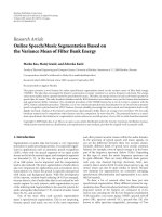
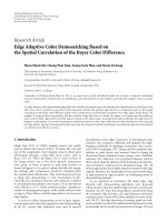
Figure 2: Generation of rough AA waves from V1 lead in an AF
episode.
where g
i
is the ith element of the global system vector g =
w
T
A, which is normalized as g
T
g = 1, and m is equal to four.
Generally speaking, an algorithm will work well if PI is less
than
−30 dB.
In each experiment (Exp
i
i = 1, 2, 3, 4), the AR model
parameters b of s
i
(i = 1, 2, 3, 4) are got using Matlab
function “aryule” with a length of p

= 20. The results are
obtained by averaging over 100 relisations, and are summa-
rized in Table 5 , which shows that ALG1 extracts the signal
with minimal MSPE, which corresponds to the analysis of
Ta ble 2 , and Ours1 extracts the one with minimal MSCPE;
meanwhile, the signal with minimal MSCPE corresponds to
the desired one in all experiments while MSPE only does in
the third and fourth experiments.
As a result, the two algorithms can both extract original
signal on the viewpoint of extracting an arbitrary signal,
but Ours1 works better than ALG1 on the viewpoint of
extracting a desired signal. It results from the fact in Tables
1–4 that the desired signal has the minimal MSCPE but not
always the MSPE.
5. ESTIMATING THE AR MODEL PARAMETERS
OF AA SOURCE
The above algorithm turns the problem of how to extract a
desired signal into that of how to estimate the corresponding
AR parameters. Then we focused the research on how to
estimate AA signal with its estimated AR parameters.
Note that Castells et al. [8, 10] have obtained the
fibrillatory wave from AF recordings by linking together
consecutive T-Q segments with no VA to synthesize AF
signal. The generation of synthesized AF ECG casts lights
upon our research. Since R wave will be easily recognized
by computer for its peak while T wave is not, and Q wave
Initialization: Obtain the roughly estimated AA as Figure 1;
Calculate the AR model parameters;
while (Error <ε, i.e., AR parameters not convergent)
Estimate AA using expression (16);

Calculate AR model parameters of the estimated AA;
Error
=AR now −AR before;
end (while)
Algorithm 1
neighbours R wave, we select the later half samples of R-R
intervals instead of T-Q intervals to generate the rough AA
and estimated its AR parameters. In order to smooth the
transitions between different intervals, we employed cubic
spline interpolation. Furthermore, clinical experience shows
that V1 lead contains the largest AA contribution among the
12-lead surface ECGs, which has been confirmed by Rieta
et al. [7] using ICA or BSS methods. Thus we would like
to select V1 lead to execute the above methods. Figure 2
illustrates how rough AA can be created from AF episode.
Initially, the coarse AR parameters are obtained using the
rough AA signal. And they would be substituted into expres-
sion (16) to extract AA signal. Then fine AR parameters
would be obtained. This calculation will not stop until the
AR parameters are convergent. Accordingly, the approaches
toextractAAinAFcanbesummarizedasinAlgorithm 1
where the operator
· denotes the Frobenius norm and ε is
the truncation error.
6. EXPERIMENTS ON REAL-WORLD
12-LEAD ELECTROCARDIOGRAM (ECG) IN
ATRIAL FIBRILLATION (AF)
The simulation in Section 4 shows that the desired signal
could be extracted if its AR parameters have been known,
and verifies expression (16). If the AR parameters might not

been known in AA case, AA source would be extracted from
real-world ECGs using Algorithm 1. For convenience, denote
Algorithm 1 with q
= 1 by Ours2.
Since AA signal has a main peak between 3.5 and 10 Hz,
and all nonrelated AA components, such as VA, have other
important spectral contents outside the band of the peak;
the spectral concentration (SC) [8, 10] around the main
frequency peak f
p
can be used as an indicator to measure
the quality of the estimated AA in real AF signal. High
Gang Wang et al. 7
150001000050000
Samples
V6 V5 V4 V3 V2 V1 aVF aVL aVR
III II I
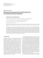
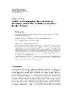
Figure 3: A 12-lead ECG segment from a patient in AF used as a
learning set.
spectral concentration values in the band of peak indicate
high quality in AA estimation. SC is defined as
SC
=

1.17 fp
0.82 fp
P
AA

f

i


fs/2
0
P
AA

f
i

×
100%, (24)
where P
AA
is the power spectrum of the AA signal.
In this experiment, twelve ECGs from eight patients
in persistent AF are tested to extract AA signal. Each lead
in every ECG contains 15000 samples (1920 samples per
second) with 16-bit amplitude. Figure 3 shows ECGs from
Patient
1
. In order to validate the AA identification, the
power spectral density (PSD) is computed for all of the
extracted signals. The procedure consists of periodogram
method with a rectangular window of 2048 points length,
a 50% overlapping between adjacent windowed section,
and an 8192-point fast Fourier transform (FFT). AR model
parameters are calculated using Matlab function “aryule”
with a length of p

= 200. AA has a main frequency peak
around 3.5–10 Hz, which is called region of interest (ROI).
Generally speaking, if the signal extracted from surface
ECGs both has a main peak between 3.5 and 10 Hz and
has an SC of more than 40%, it could be regarded as AA
signal.
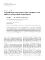
Figure 4(b) plots one extracted AA from ECG
1
/Patient
1
,
and Figure 4(a) shows the corresponding PSD along with
the atrial frequency, where the spectral content above 2 Hz
is discarded due to its low contribution. The extracted one
canberegardedasAAsignal,forthatithasonlyonepeak
frequency in ROI, and its SC is more than 40%.
Comparisons are done among ALG1, ALG2, and Ours2
algorithms, and the AR parameters used in ALG1 would be
obtained from the extracted AA by ALG2. The applications of
the three algorithms on the twelve real ECGs are summarized
2520151050
Frequency (Hz)
PSD
Fp = 7.5Hz
SC
= 70.7712%
(a)
150001000050000
Samples
−5

0
5
(b)
Figure 4: (a) The extracted AA signal from patient one; (b) The
corresponding PSD along with the atrial frequency.
20151050
Iterate number
0
0.5
1
1.5
2
2.5
3
3.5
Errors during iterations
Figure 5: The learning curve of Algorithm 1.
in Ta ble 6 . It shows that none of the signals extracted by
ALG1 has an SC of more than 40%. The main frequencies of
atrial wave extracted by Ours2 range from 4.7 to 8.4 Hz, and
the SC is 53.97% on average. The main frequencies extracted
by ALG2 are from 4.7 to 8.4 Hz, and the SC is 50.91%
on average. These results demonstrate that the proposed
algorithm is as efficient as ICA method, but the algorithm
based on linear predictor fails to extract AA signal. Figure 5
plots the averaged learning curve of Ours2 for the twelve
extractions. All of the twelve extractions are converged in
8 EURASIP Journal on Advances in Signal Processing
Table 6: Experiments of ALG1, ALG2, and Ours2.
ECG

i
/Patient
j
SC of ALG1 (%) SC of ALG2 (%) SC of Ours2 (%) Fp of ALG1 (Hz) Fp of ALG2 (Hz) Fp of Ours2 (Hz)
i = 1/j = 1 24.8519 66.8203 70.7712 4.2353 7.5000 7.5000
i
= 2/j = 1 25.9875 58.7091 62.1591 2.8125 7.5000 7.5000
i
= 3/j = 2 19.1397 51.0525 50.4415 1.8750 5.6250 5.6250
i
= 4/j = 2 23.2529 50.7547 52.2671 3.7500 7.5000 7.5000
i
= 5/j = 3 16.6486 55.9363 59.9669 0.9375 4.6875 4.6875
i
= 6/j = 3 16.7755 57.9015 59.3211 1.8750 4.6875 4.6875
i
= 7/j = 4 16.1763 48.4142 46.8586 2.8125 6.5625 6.5625
i
= 8/j = 4 10.4663 38.1165 44.5730 3.7500 6.5625 6.5625
i
= 9/j = 5 22.3358 44.7337 48.2786 1.8750 8.4375 8.4375
i
= 10/j = 6 32.3524 43.1452 46.6405 3.7500 7.5000 7.5000
i
= 11/j = 7 14.2147 47.3161 55.4149 0.9375 4.6875 4.6875
i
= 12/j = 8 14.9846 48.0524 59.1223 1.8750 5.6250 5.6250
Mean 19.7655 50.9127 54.6513 2.5404 6.4063 6.4063
150001000050000
Samples

EEG
12
EEG
11
EEG
10
EEG
9
EEG
8
EEG
7
EEG
6
EEG
5
EEG
4
EEG
3
EEG
2
Figure 6: AA extraction results from ECG
2
–ECG
12
. It shows the
extracted AA source (top) and lead V1 (bottom).
ten iterations. Moreover, the BSE-based algorithm needs less
computation than ICA.

In the twelve ECGs, the former eight are divided into four
different groups, which come from four different patients,
and each group contains two ECGs. The extracted results in
Ta ble 6 show that different ECGs from the same patient (e.g.,
patient
2
) sometimes have different main frequencies, which
verifies that AA is nonstationary in long term.
The visual comparisons between the extracted signals
and the AA present in the original ECG are summarized in
Figure 6, which provided satisfactory results. These results
12-lead ECG
Separated signals
Noise
PCA/ICA
Peak in
3–10 Hz
No
Yes AF signal
Figure 7: The frame based on ICA or PCA.
12-Lead ECG
Extracted
signal
AF is off
BSE
Peak in
3–10 Hz
No
Ye s
AF is on

Figure 8:ThenewframebasedonBSE.
correspond to ECG
2
–ECG
12
. In the figure, lead V1 (in the
bottom) can be observed from the 12-lead ECG in AF, along
with the Ours2-estimated AA for that episode (at the top) for
visual comparison. The estimated AA has been scaled by the
factor associated with its projection onto lead V1.
7. DISCUSSION AND CONCLUSIONS
In this paper, we propose an efficient semi-BSE algorithm
based on AR model parameters to extract a specific signal.
The algorithm transforms the problem on how to extract a
specific signal into that on how to estimate its AR model,
and is verified by the theoretical analysis and computer
simulations. The algorithm embodies the desired property,
and it can be used in related fields where the AR parameters
of the desired signal can be approximately estimated before
extraction. On this standpoint this algorithm is more robust
than the ones based on linear predictor [19]. Moreover, this
algorithm can be regarded as an extension of the algorithm
in [19], when the time delay q is equal to zero.
Gang Wang et al. 9
The expression (16) showed that the proposed algorithm
relates to minor component analysis (MCA). Thus, many
results [11, 23] on MCA can be used to improve the
algorithm, which will be our future work.
From the methodological standpoint, we propose an-
other BSE-based algorithm to extract AA signal except pri-

mary component analysis (PCA), ICA, and spatiotemporal
QRST cancellation (STC) methods [5].
STC techniques obtained as many AA signals as leads
processed by the cancellation algorithm. In contrast, the
ICA/PCA-based approaches estimate a single signal, which
is able to reconstruct the complete AA present in every
ECG lead, thus the two methods are more robust than STC
method. Figure 7 describes the frame of ICA/PCA method,
and shows that ICA/PCA method cannot directly extract
the AF signal; power spectrum analysis will be utilized to
tell which one is AF signal by judging whether the signal
has a peak in 3–10 Hz. As a contrast, the BSE-based frame
shown in Figure 8 [24] only extracts one signal, thus it has
lower computational load than Figure 7, need only one-
twelfth memory of ICA/PCA method, and it is more suitable
in clinical monitoring. The proposed algorithm could be
applied into this frame and will have great potential in
clinical monitoring machine.
ACKNOWLEDGMENTS
This work is supported by National Nature Science Foun-
dation 60571047. The authors wish to thank the National
project for postgraduates of key constructed high-level
universities in China in 2007.
REFERENCES
[1] J. S. Steinberg, S. Zelenkofske, S C. Wong, M. Gelernt, R.
Sciacca, and E. Menchavez, “Value of the P-wave signal-
averaged ECG for predicting atrial fibrillation after cardiac
surgery,” Circulation, vol. 88, no. 6, pp. 2618–2622, 1993.
[2] R. G. Tieleman, I. C. Van Gelder, H. J. G. M. Crijns,
et al., “Early recurrences of atrial fibrillation after electri-

cal cardioversion: a results of fibrillation-induced electrical
remodeling of the atria?” Journal of the American College of
Cardiology, vol. 31, no. 1, pp. 167–173, 1998.
[3] O.D.Escoda,L.Granai,M.Lemay,J.M.Hernandez,P.Van-
dergheynst, and J M. Vesin, “Ventricular and atrial activity
estimation through sparse ECG signal decompositions,” in
Proceedings of the IEEE International Conference on Acoustics,
Speech and Signal Processing (ICASSP ’06), vol. 2, pp. 1060–
1063, Toulouse, France, May 2006.
[4] J. J. Rieta and F. Hornero, “Comparative study of methods
for ventricular activity cancellation in atrial electrograms of
atrial fibrillation,” Physiological Measurement, vol. 28, no. 8,
pp. 925–936, 2007.
[5]M.Lemay,V.Jacquemet,A.Forclaz,J.M.Vesin,andL.
Kappenberger, “Spatiotemporal QRST cancellation method
using separate QRS and T-waves templates,” in Proceedings
of Computers in Cardiology, pp. 611–614, Lyon, France,
September 2005.
[6]J.J.Rieta,F.Hornero,C.S
´
anchez, C. Vay
´
a, D. Moratal,
and J. M. Sanchis, “Derivation of atrial surface reentries
applying ICA to the standard electrocardiogram of patients
in postoperative atrial fibrillation,” in Proceedings of the 6th
International Conference on Independent Component Analysis
and Blind Signal Separation (ICA ’06), vol. 3889, pp. 478–485,
Charleston, SC, USA, March 2006.
[7]J.J.Rieta,F.Castells,C.S

´
anchez, V. Zarzoso, and J. Millet,
“Atrial activity extraction for atrial fibrillation analysis using
blind source separation,” IEEE Transactions on Biomedical
Engineering, vol. 51, no. 7, pp. 1176–1186, 2004.
[8] F. Castells, J. J. Rieta, J. Millet, and V. Zarzoso, “Spatiotemporal
blind source separation approach to atrial activity estimation
in atrial tachyarrhythmias,” IEEE Transactions on Biomedical
Engineering, vol. 52, no. 2, pp. 258–267, 2005.
[9] P. Langley, J. J. Rieta, M. Stridh, J. Millet, L. Sornmo, and A.
Murray, “Comparison of atrial signal extraction algorithms
in 12-lead ECGs with atrial fibrillation,” IEEE Transactions on
Biomedical Engineering, vol. 53, no. 2, pp. 343–346, 2006.
[10]F.Castells,J.Igual,J.Millet,andJ.J.Rieta,“Atrialactivity
extraction from atrial fibrillation episodes based on maximum
likelihood source separation,” Signal Processing, vol. 85, no. 3,
pp. 523–535, 2005.
[11] A. Cichocki and S. B. Amari, Adaptive Blind Signal and Image
Processing: Learning Algorithms and Applications,JohnWiley
& Sons, Chichester, UK, 2002.
[12] A. Hyv
¨
arinen, J. Karhunen, and E. Oja, Independent Compo-
nent Analysis, John Wiley & Sons, Chichester, UK, 2001.
[13] Z L. Zhang and Z. Yi, “Robust extraction of specific signals
with temporal structure,” Neurocomputing, vol. 69, no. 7–9,
pp. 888–893, 2006.
[14] W. Lu and J. C. Rajapakse, “Approach and applications of
constrained ICA,” IEEE Transactions on Neural Networks, vol.
16, no. 1, pp. 203–212, 2005.

[15] A. Cichocki, R. Thawonmas, and S. Amari, “Sequential blind
signal extraction in order specified by stochastic properties,”
Electronics Letters, vol. 33, no. 1, pp. 64–65, 1997.
[16] A. K. Barros and A. Cichocki, “Extraction of specific signals
with temporal structure,” Neural Computation,vol.13,no.9,
pp. 1995–2003, 2001.
[17] W. Liu, D. P. Mandic, and A. Cichocki, “Blind second-order
source extraction of instantaneous noisy mixtures,” IEEE
Transactions on Circuits and Systems II
, vol. 53, no. 9, pp. 931–
935, 2006.
[18] A. Cichocki and R. Thawonmas, “On-line algorithm for blind
signal extraction of arbitrarily distributed, but temporally cor-
related sources using second order statistics,” Neural Processing
Letters, vol. 12, no. 1, pp. 91–98, 2000.
[19] W. Liu, D. P. Mandic, and A. Cichocki, “Blind source
extraction based on a linear predictor,” IET Signal Processing,
vol. 1, no. 1, pp. 29–34, 2007.
[20] M. Holm, S. Pehrson, M. Ingemansson, et al., “Non-invasive
assessment of the atrial cycle length during atrial fibrillation
in man: introducing, validating and illustrating a new ECG
method,” Cardiovascular Research, vol. 38, no. 1, pp. 69–81,
1998.
[21] P. Langley, J. P. Bourke, and A. Murray, “Frequency analysis of
atrial fibrillation,” in Proceedings of Computers in Cardiology,
pp. 65–68, Cambridge, Mass, USA, September 2000.
[22] A. Hyv
¨
arinen, “Fast and robust fixed-point algorithms for
independent component analysis,” IEEE Transactions on Neu-

ral Networks, vol. 10, no. 3, pp. 626–634, 1999.
[23] E. Oja, “Principal components, minor components, and linear
neural networks,” Neural Networks, vol. 5, no. 6, pp. 927–935,
1992.
[24] G. Wang, N. Rao, and Y. Zhang, “Atrial fibrillatory signal
estimation using blind source extraction algorithm based on
high-order statistics,” to appear in Science in China, Series F.