Báo cáo hóa học: " Research Article Blind Channel Equalization with Colored Source Based on Constrained Optimization Methods" pptx

Hindawi Publishing Corporation
EURASIP Journal on Advances in Signal Processing
Volume 2008, Article ID 960295, 9 pages
doi:10.1155/2008/960295
Research Article
Blind Channel Equalization with Colored Source Based
on Constrained Optimization Methods
Yunhua Wang,
1
Linda DeBrunner,
2
Victor DeBrunner,
2
and Dayong Zhou
3
1
Department of Electrical and Computer Engineering, Oklahoma University, Norman, OK 73072, USA
2
Department of Electrical and Computer Engineering, Florida State University, Tallahassee, FL 32306, USA
3
Cirrus Logic Inc., 2901 Via Fortuna, Austin, TX 78746, USA
Correspondence should be addressed to Dayong Zhou,
Received 20 February 2008; Revised 23 June 2008; Accepted 11 September 2008
Recommended by Magnus Jansson
Tsatsanis and Xu have applied the constrained minimum output variance (CMOV) principle to directly blind equalize a linear
channel—a technique that has proven effective with white inputs. It is generally assumed in the literature that their CMOV method
can also effectively equalize a linear channel with a colored source. In this paper, we prove that colored inputs will cause the
equalizer to incorrectly converge due to inadequate constraints. We also introduce a new blind channel equalizer algorithm that is
based on the CMOV principle, but with a different constraint that will correctly handle colored sources. Our proposed algorithm
works for channels with either white or colored inputs and performs equivalently to the trained minimum mean-square error
(MMSE) equalizer under high SNR. Thus, our proposed algorithm may be regarded as an extension of the CMOV algorithm

proposed by Tsatsanis and Xu. We also introduce several methods to improve the performance of our introduced algorithm in the
low SNR condition. Simulation results show the superior performance of our proposed methods.
Copyright © 2008 Yunhua Wang et al. This is an open access article distributed under the Creative Commons Attribution License,
which permits unrestricted use, distribution, and reproduction in any medium, provided the original work is properly cited.
1. INTRODUCTION
In digital communication, the multipath effect in a channel
will subject the signal to intersymbol interference (ISI). The
ISI will increase the symbol error rate (SER) at the receiver,
sometimes making a correct estimation of the sent signal
impossible. As a result, equalizers are required to remove
the channel distortion. Roughly speaking, two kinds of
equalizers in digital communication systems exist: data aided
(trained) equalizers and blind equalizers. For data aided
equalizers, a reference signal is required, increasing the data
bandwidth. As a result, a blind equalizer is preferred in high-
speed communication systems due to its potential to reduce
the ISI without increasing the overhead costs.
Blind channel equalization relies solely on the channel
output, with/without some a priori statistical knowledge
of the input of the channel. Blind system equalization for
a single input can be divided into two categories: single
input single output (SISO) configurations, for example,
the constant modulus algorithm (CMA), and single input
multiple output (SIMO) configurations. Note that all SISO
blind identification and equalization algorithms explicitly or
implicitly exploit the high-order statistics of the input and
output signals. As a result they all suffer from local minima
or slow convergence [1, 2].
The SIMO configuration can be obtained from the
exploitation of temporal (oversampling) or spatial (multi-

antenna) diversity of the received signal. The TXK algorithm
developed by Tong et al. [3] first proved that the channel
information could be blindly estimated using only second-
order statistics by exploiting the diversity. Different SIMO
blind channel estimation and equalization algorithms have
been proposed, such as the subchannel matching algorithm
[4], the subspace algorithm [5], the linear prediction algo-
rithm [6, 7], adaptive least square smoothing [8], and the
outer product decomposition algorithm [9, 10] (some details
about these and other algorithms can be found in [1] and its
references). The popularity of SIMO, rather than SISO, blind
channel identification and equalization comes from the fast
convergence and efficient computation of these algorithms.
Most of the SIMO-based blind channel estimation and
equalization methods assume that the channel input is
white; as a result, the designed equalizers are sensitive to
the color of the input. One could use a whitening filter
2 EURASIP Journal on Advances in Signal Processing
to prewhiten the colored source before transmission; then
use channel equalization for white sources to remove the
channel effect; and then finally inverse filter to recover
the original source. However, sometimes this complicated
process may not be possible due to the inaccessibility of
the input or the unavailability of the exact inverse filter; in
any case, the prewhitening and inverse processes complicate
the overall system required in this approach. Consequently,
several researchers, such as L
´
opez-Valcarce and Dasgupta
and Afkhamie and Luo, have attempted to extend the TXK

method to solve the colored input problem ([11, 12], resp.),
but the algorithms either entail many restrictions or have
a large computational burden. Some SIMO-based blind
channel equalization methods do not require assumptions
regarding the input statistics, so they can be applied to
systems with either white or colored inputs. For example,
the subspace-based method introduced by Moulines et al.
[5] could work for colored inputs. However, usually, the
equalizer design requires a two-step procedure—the first step
is to estimate the channel coefficients while the second step
is to invert the channel effects using either zero forcing or an
MMSE equalizer. Moreover, these methods do not exploit the
input statistics—something that is already known to improve
equalizer performance [11], though at a cost of increasing
computational complexity.
Tsatsanis and Xu [13] proposed a direct blind equal-
ization method by incorporating the constrained minimum
output variance (CMOV), which is widely used in array sig-
nal processing. Based on their algorithm, the blind equalizer
achieves a performance close to the trained MMSE equalizer
for channels with white inputs at high SNR. The introduced
Tsatsanis and Xu’s (TX’s) CMOV algorithm obtains the
channel information from the noise subspace [13, 14]. As a
result, this algorithm can be regarded as a subspace method.
However, unlike the subspace method discussed in [5], the
TX’s CMOV-based algorithm requires less computational
complexity. Furthermore, using the CMOV principle, an
adaptive blind channel equalization algorithm has been
developed in [15]. However, the TX’s CMOV algorithm does
not work for colored input, though it is believed to work in

this case; see, for example, [1, 13].
Colored sources may occur, for example, as a result of
channel encoding. Under this situation, the knowledge of
the encoding scheme alone will provide the required source
statistics to the receiver [16]. In this work, we develop a
new blind channel equalizer for channels with colored inputs
based on the known source second-order statistics. Note
that our developed method is different from both semiblind
channel estimation which assumes additional knowledge of
the symbol, and trained equalization which requires training
sequences. By contrast, in our configuration, no training
sequences are required, and only the second-order statistical
information of the input is available to the receiver.
The contributions of this paper are two-fold. First, we
point out and correct a widely-held misunderstanding about
the previous developed CMOV-based channel equalization
algorithm. Second, we extend the application of the CMOV
principle by finding a new constraint and develop an efficient
blind channel equalization method that works for both
colored and white inputs. A part of these research results
has been presented in [17]. In our notation, the superscripts
(
·)
∗
,(·)
T
,and(·)
H
denote, respectively, the conjugate, the
transpose, and the Hermitian transpose, and E(

·)denotes
expected value.
2. PROBLEM DEFINITION
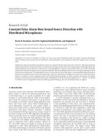
Figure 1 shows the baseband representation of an SIMO data
communication system with input s(k).Theleftsideofthe
figure represents the multichannels h
i
(k) with multiple mea-
surements x
i
(k) while the right represents the multichannel
equalizer g
i
(k) with output y(k). The signals n
i
(k)arewhite
noise. There are p channels in Figure 1 SIMO configuration.
The SIMO channel in vector form is
x(k) =
q

i=0
h(i)s(k − i)+n(k)(1)
with
h(i)
Δ
=
⎡
⎢
⎢

⎣
h
1
(i)
.
.
.
h
p
(i)
⎤
⎥
⎥
⎦
, x(k)
Δ
=
⎡
⎢
⎢
⎣
x
1
(k)
.
.
.
x
p
(k)

⎤
⎥
⎥
⎦
, n(k)
Δ
=
⎡
⎢
⎢
⎣
n
1
(k)
.
.
.
n
p
(k)
⎤
⎥
⎥
⎦
.
(2)
Here, we denote the ith term of the finite impulse response
(FIR) of jth channel as h
j
(i). We use the symbol q to denote

the order of the channel response. Equation (1)canbe
rewritten as
x(k)
= T(h)s(k)+n(k)(3)
using the following definitions:
s(k)
Δ
=
⎡
⎢
⎢
⎣
s(k)
.
.
.
s(k
− q − M)
⎤
⎥
⎥
⎦
, x(k)
Δ
=
⎡
⎢
⎢
⎣
x(k)

.
.
.
x(k − M +1)
⎤
⎥
⎥
⎦
,
n(k)
Δ
=
⎡
⎢
⎢
⎣
n(k)
.
.
.
n(k − M +1)
⎤
⎥
⎥
⎦
,
T(h)
=
⎡
⎢

⎢
⎢
⎢
⎢
⎣
h(0) h(1) ··· h(q) 0 ··· 0
0h(0)
.
.
.
··· h(q)
.
.
.
0
.
.
.
.
.
.
.
.
.
.
.
.
.
.
.

00
··· h(0) h(1) ··· h(q)
⎤
⎥
⎥
⎥
⎥
⎥
⎦
⎫
⎪
⎪
⎪
⎪
⎪
⎪
⎬
⎪
⎪
⎪
⎪
⎪
⎪
⎭

 
M+q
Mp,
(4)
where M is the number of taps in the FIR equalizer g

i
(k)and
T(h)isanMp
× (M + q) block Toeplitz matrix. We denote
the ith column of T(h)byh
i
, that is,
T(h)
=

h
1
, h
2
, , h
M+q

. (5)
We define the channel coefficient vector as
h
=

h
T
(q) h
T
(q − 1) ··· h
T
(0)


T
. (6)
Yunhua Wang et al. 3
s(k)
y(k)
h
1
(n)
h
2
(n)
h
p
(n)
g
1
(n)
g
2
(n)
g
p
(n)
Channel
Channel
Channel
Equalizer
Equalizer
Equalizer
y

1
(k)
y
2
(k)
y
p
(k)
x
1
(k)
x
2
(k)
x
p
(k)
n
1
(k)
n
2
(k)
n
p
(k)
+
+
+
+

.
.
.
.
.
.
Figure 1: SIMO blind channel estimation and equalization.
Equations (5)and(6) will be useful in the following
discussion. Our problem is to find g
i
(k) based on the
following assumptions:
(AS1) the input s(k) is unknown, but the second-order
statistic E(s(k)s
H
(k)) is known and has full rank;
(AS2) T(h) has full column rank, that is, the Z-transforms
of the h
j
(1 ≤ j ≤ M + q) have no common zero;
(AS3) measurement noise n
i
(k) is independent and identi-
cally distributed (iid) zero mean noise with variance
σ
2
n
.
These are common assumptions in multichannel blind
identification and equalization problems [5–10, 12]. For

instance, note that (AS1) has been used in [11] to extend the
TXK method for colored input.
In the same manner that we defined the vector structure
in (3), we define the equalizer g as follows:
g(i)
Δ
=

g
1
(i), g
2
(i), , g
p
(i)

T
,
g
Δ
=

g
T
(0), g
T
(1), , g
T
(M − 1)


T
,
(7)
where g
j
(i) denotes the ith term of the jth FIR equalizer. We
want the output of the equalizer to be an undistorted version
of the input, that is, we allow
y(k)
= g
H
x(k) = g
H
T(h)s(k) = s(k − d), (8)
where d is some integer. For the trained MMSE equalizer [18]
g
MMSE
= R
−1
x
E

x(k)s(k − d)

=
R
−1
x
T(h)E


s(k)s
∗
(k − d)

,
(9)
where R
x
is the channel output covariance matrix
R
x
= E

x(k)x
H
(k)

. (10)
Note if the source is white, the autocorrelation of the source
becomes a delta function. Therefore, the MMSE equalizer for
white input becomes
g
MMSE
= R
−1
x
h
d+1
. (11)
From (9), we see that to determine the MMSE equalizer,

we must have the channel coefficient matrix and source
signal second-order statistics. However, for our problem, the
channel matrix T(h) is not available. We desire to find a blind
equalizer g with performance close to g
MMSE
that works for
both white and colored inputs.
3. ANALYSIS OF EXISTING CMOV METHOD
Tsatsanis and Xu [13], borrowing from work in array signal
processing, proposed a CMOV method which successfully
solves the above problem when the input s(n) is white and the
SNRofthemeasuredx(n) is high. The equalizer is developed
using the constrained optimization:
arg min
g
E



y(k)


2

=
min
g
g
H
R

x
g with g
H
h
d+1
= 1.
(12)
h
d+1
is defined in (5). Using the method of Lagrange, the
equalizer g is
g
TX
=

h
H
d+1
R
−1
x
h
d+1

−1
R
−1
x
h
d+1

. (13)
Note that for a white input, the equalizer in (13) only has an
amplitude difference from an optimum MMSE equalizer in
(11). We can obtain the minimum output variance which is
V
min
=

h
H
d+1
R
−1
x
h
d+1

−1
. (14)
However in blind channel equalization, the channel infor-
mation h
d+1
is unknown. Tsatsanis and Xu resorted to the
Capon max/min approach [19] to estimate the channel
response h. This approach may be succinctly described.
Define the structure matrix C
d+1
C
d+1
=


0
p(d−q)×p(q+1)
I
p(q+1)×p(q+1)
0
p(M−d−1)× p(q+1)

H
(15)
and channel coefficients vector h as in (6) so that
h
d+1
= C
d+1
h (16)
for M
≥ d +1≥ q + 1. The estimated h is then obtained by
maximizing the minimum output variance in (14), that is,

h = arg max
h
h
H
C
H
d+1
C
d+1
h

h
H
C
H
d+1
R
−1
x
C
d+1
h
= arg min
h
h
H
C
H
d+1
R
−1
x
C
d+1
h
h
H
h
.
(17)
4 EURASIP Journal on Advances in Signal Processing

Of course, the solution is the eigenvector corresponding to
the minimum eigenvalue of C
H
d+1
R
−1
x
C
d+1
.Theproofin[13]
shows that

h =
h
h
as σ
2
n
−→ 0. (18)
Using this estimated

h, one can now compute the CMOV
equalizer directly using (13). Note that the algorithm
developed by Tsatsanis and Xu requires that the order of the
equalizer must be above 3(q+1), and“d is not allowed to take
any of the first or last 2q allowable lag[s].” These restrictions
ensure that (18)holds.
It is believed that the above “are not sensitive to the
color of the input” [13]. However, our simulations (refer
to Section 7) show that the algorithm fails to generate a

correct equalizer for a channel with colored input. Since the
estimation of

h and the proof of (18)donotrequirewhite
input, the estimation of the channel will not be affected by
colored inputs. However, the very basis of the constrained
optimization (12) will generate a biased equalizer in this
case, which means the equalizer calculated by (13) cannot
eliminate the channel effect for nonwhite inputs. The reason
for the failure of the CMOV method is its inadequate
constraints.
These inadequacies can be illustrated using the overall
channel response model of Figure 1. The combined response
of the p channels and p equalizers can be regarded as an SISO
FIR filter f (n)withorderM+q. We want the overall response
of the channel and equalizer, f (n), to be only delay, and so
only one coefficient of f (n) can be nonzero. The coefficient
vector of f (n)is
f
= g
H
T(h) =

g
H
h
0
, g
H
h

1
, , g
H
h
d+1
, , g
H
h
M+q

.
(19)
The variance of the output of this FIR filter is
γ
y
(0) =
M+q

l=0
M+q
−1

m=0
γ
s
(m − l) f
H
(m)
= fR
s

f
H
,
(20)
where r
s
(n) = E[s(k)s
∗
(k − n)] and R
s
is the autocorrelation
matrix of input signal s(k). For white inputs,
r
y
(0) = r
s
(0)
M+q−1

n=0
 f (n)
2
. (21)
Using the constraint f (d)
= g
T
h
d+1
= 1
/

= 0, the minimum
output variance is achieved when all coefficients in f are
zero except f (d), that is, the filter f (n) is a delay of d
samples. However, for colored inputs, minimizing r
y
(0) with
the constraint g
T
h
d+1
= 1 cannot guarantee that f (n)will
converge to a pure delay. Actually, the overall response f (n)
will force the frequency component of y(n) to be the one’s
complement of the input signal s(n), which is easily obtained
by analyzing g
TX
in (13)[20].
4. DEVELOPMENT OF OUR NEW CMOV ALGORITHM
From our previous analysis, we find that the TX’s CMOV
method cannot correctly equalize a linear channel for colored
input due to the inadequate constraint that causes the
equalizertoconvergetoabiasedvalue.Tofindagood
equalizer based on the CMOV method is then to find an
efficient constraint that forces the overall response f (n)in
(19) to be a simple delay. In this section, we first find this
efficient constraint based on the overall response analyses in
the previous section. Then we develop a new equalization
algorithm based on the CMOV method that successfully
removes the channel effects.
4.1. An efficient constraint for colored input

In CMOV-based equalization methods, the constraint plays
a very important role. An efficient constraint should not only
prevent the signal from being eliminated, but it should also
guarantee the removal of the ISI. For our purposes, we define
the efficient constraint mathematically in the following.
Definition 1. Consider the constraint fγ
= 1,whereγ is a
vector of length M + q. If, using this constraint, the solution
of arg min
f
fR
s
f
H
is
f
=

0 ···0
  
d−1
10···0

, (22)
then we say this constraint is an efficient constraint.
In this definition, vector f is the coefficient vector of the
overall channel response defined in (19). The vector γ can
be found using Lagrange multipliers. We first define a cost
function
E

1
2
fR
s
f
H
+ λ

1 − fγ
H

. (23)
Differentiating the right side of (23)withrespecttof, the
minimum achieved at ∂E/∂f
= 0 yields
∂E
∂f
= R
s
f
H
− λγ = 0,
γ
=
1
λ
R
s
f
H

.
(24)
Note that R
s
is invertible based on (AS1). Considering
f
=

0 ···0
  
d−1
10···1

, (25)
we find that γ should be the dth column of the input
correlation matrix, that is,
γ
=
1
λ
E

s(k)s
∗
(k − d)

=
1
λ


r
s
(d),r
s
(d − 1), , r
s
(0), , r
s
(M + q − d − 1)

H
(26)
which of course is the correlation between the delayed input
and the input vector. Based on (26)andDefinition 1,we
Yunhua Wang et al. 5
can have the efficient constraint fγ = 1, so that the overall
response f (n) can be guaranteed to be only a delay. As
a result, using this constraint, we can successfully reduce
the ISI caused by a channel. Note that we do not consider
the measurement noise in finding the efficient constraint.
However, we prove next that the blind equalizer we develop
in this paper is an MMSE-like equalizer instead of zero force
(ZF) equalizer.
4.2. New CMOV-based blind channel equalizer
Based on the efficient constraint developed in the previous
subsection, we first prove the following proposition before
we introduce our new CMOV-based blind channel equaliza-
tion method.
Proposition 1. If g
H

= arg min
g
H
E {y (k) 
2
}=
arg min
g
H
g
H
R
x
g with g
H
T(h)γ = 1, then this solution differs
from the MMSE equalizer only by a scalar factor gain.
Proof. This is a constrained optimization problem, which
can also be solved using Lagrange multipliers. First define the
cost function
J
=
1
2
g
H
R
x
g + λ


1 − g
H
T(h)γ

. (27)
Again, we use λ as the Lagrange multiplier. Minimizing the
cost function yields
λ
=

γ
H
T(h)
H
R
−1
x
T(h)γ

−1
,
(28)
g
H
=
R
−1
x
T(h)γ
γ

H
T(h)
H
R
−1
x
T(h)γ
.
(29)
Comparing (29)with(9), we see only a scalar factor
difference between g
H
and the MMSE equalizer.
Note that the similar CMOV concept has been applied
in multiuser detection and array signal processing [21].
Proposition 1 provides the theoretical background of our
new algorithm. However, as with the method in TX [13], this
constrained optimization requires channel information that
is not available. In order to estimate the channel information,
we need to resort to the Capon max/min method.
The minimum output variance is obtained when g
H
takes
the value in (29)
V
min

g
H


=

γ
H
T(h)
H
R
−1
x
T(h)γ

−1
. (30)
Based on the Capon max/min method, we can find the
channel information by maximizing the minimum output
variance V
min
(g
H
). However, it is not easy to directly apply
the max/min method. We define an extension of the vector γ
γ
ext
=

0, ,0
  
p−1
, γ(M+q), 0, ,0
  

p−1
, γ(M+q−1), , γ(1), 0, ,0
  
p−1

H
.
(31)
Note that this extended vector is constructed by reversing the
vector γ and interspersing p
−1 zeros between every element.
Then we construct the pM
× p(q + 1) Toeplitz matrix T(γ
ext
)
of this γ
ext
as
T

γ
ext

=
⎡
⎢
⎢
⎢
⎢
⎢

⎣
γ
H
ext
(pM : pM + pq + p − 1)
γ
H
ext
(pM − 1:pM + pq + p − 2)
.
.
.
γ
H
ext

1:p(q +1)

⎤
⎥
⎥
⎥
⎥
⎥
⎦
. (32)
Lemma 1. The following relation holds
T(h)γ
= T


γ
ext

h. (33)
This lemma can be proven by direct substitution or using
a method based on the Z-transform [5]. One anonymous
reviewer als o pointed out that this is commutative property of
convolution in a matrix formulation. Using (31) and Lemma 1,
we rewrite (30) as
V
min

g
H

=

h
H
T

γ
ext

H
R
−1
x
T


γ
ext

h

−1
. (34)
At this point, we can apply the Capon max/min principle to
estimate h
h
capon
= arg max
h

h
H
T

γ
ext

H
R
−1
x
T

γ
ext


h

−1
= arg min
h
h
H
T

γ
ext

H
R
−1
x
T

γ
ext

h.
(35)
We see that
h
capon
is equal to the eigenvector corresponding to
the minimum eigenvalue of T(γ
ext
)

H
R
−1
x
T(γ
ext
). Thus, our
algorithm for blind channel equalizer design can be summa-
rized in the following steps:
(1) obtain the source statistics
γ
ext
and R
−1
x
;
(2) construct T(γ
ext
) and A = T(γ
ext
)
H
R
−1
x
T(γ
ext
);
(3) estimate the channel
h

capon
coefficient by finding the
minimum eigenvalue and corresponding eigenvector of
A;
(4) find the equalizer g
H
= R
−1
x
T(γ
ext
)h
capon
;
(5) remove the phase ambiguity which is inhe rent to all
SOS-based method.
5. CONVERGENCE ANALYSIS
The main difference between our proposed CMOV algo-
rithm and TX’s CMOV algorithm is the different constraint.
We already proved that TX’s CMOV algorithm cannot
generate an adequate equalizer for colored input due to its
inadequate constraint. In this section, we will see that our
proposed blind equalizer converges to trained MMSE equal-
izer for high SNR systems following the similar convergence
analyses approach in [13].
As shown in (29) and step (4) of our algorithm, if the
estimated
h
capon
is equal to the correct channel coefficient

vector h, then the blind equalizer differs from the MMSE
6 EURASIP Journal on Advances in Signal Processing
equalizer only by a scale factor. The scale can be corrected
by comparing the power of the equalizer output and the
system input. Consequently, our developed equalizer will
have equivalent performance to the trained MMSE equalizer.
As a result, how well the estimated channel coefficients vector
relates to the true vector will determine the performance of
the proposed equalizer. To see this, we need to prove the
following proposition.
Proposition 2. If the order of the equalizer M
≥ (p + qp +
q)/(p
−1) and the number of delays d satisfy the constraint M−
(p+q)/(p−1) ≥ d ≥ pq/(p−1), as the SNR →∞,the
h
capon
estimated in (35) differs from the true channel coefficients by a
phase and scale factor, that is,
h
capon
=
e
jθ
h
h
as σ
2
n
−→ 0. (36)

Proof. We follow the same steps as in [13], that is, we first
prove h is a solution of arg min
h
h
H
T(γ
ext
)
H
R
−1
x
T(γ
ext
)h as
σ
2
n
→ 0. We then prove this solution is unique within a scalar
constant under the condition given by Proposition 2.
Step 1. We first write the eigen-decomposition of R
x
:
R
x
=

V
s
V

n


Λ
s
0
00

V
H
s
V
H
n

+ σ
2
n
I, (37)
where
Λ
s
= diag{λ
1
, , λ
M+q
} and where
V
s
and

V
n
represent the signal and noise subspaces, respectively. It has
been proved in [13, equation (32)] that
σ
2
n
C
H
d+1
R
−1
x
C
d+1
−→ C
H
d+1
V
n
V
H
n
C
d+1
(38)
as σ
2
n
→ 0. Similarly we can have

σ
2
n
A = σ
2
n
T

γ
ext

H
R
−1
x
T

γ
ext

−→
T

γ
ext

H
V
n
V

H
n
T

γ
ext

(39)
as σ
2
n
→ 0. So, the eigenvectors of A form the noise
subspace. Because the signal subspace V
s
is orthogonal to
the noise subspace and T(γ
ext
)h = T(h)γ ∈ V
s
,weget
V
H
n
T(γ
ext
)h = 0. Consequently, we find that h is a solution
of arg min
h
h
H

T(γ
ext
)
H
R
−1
x
T(γ
ext
)h.
Step 2. Prove under the above conditions that h is the only
solution of arg min
h
h
H
T(γ
ext
)
H
R
−1
x
T(γ
ext
)h.Itisequivalent
to prove that there is no other vector h

with h

/

= ch (c a
complex constant), so that T(γ
ext
)h

∈ V
s
.
This step is proven by contradiction. Assume that we
have T(γ
ext
)h

∈ V
s
. Then
T

γ
ext

h

= T

h


γ ∈ V
s

. (40)
Consequently,
T

h


γ = T(h)θ, (41)
where θ is a (M + q)
× 1 vector and the elements in θ are
unknown constants. We need to prove that (41) has only one
set of solutions θ and T(h

). Equation (41)isasetoflinear
equations with M+q+ p(q+1) unknowns and Mpequations
when every component of γ is nonzero. Considering T(h)
has full column rank, we only need the number of equations
to be greater than or equal to the number of unknowns to
ensure there is a unique solution. Consequently, we find that
the order of the blind nonlinear equalizer is
M
≥
p + qp+ q
p − 1
. (42)
This condition shows that increasing the number of channels
will reduce the requirements on the order of the equalizer.
Furthermore, to successfully equalize the channel, we need
at least two channels, that is, p
≥ 2.

When the input is white noise, the ideal γ has only one
nonzero component. Combining this fact with the Toeplitz
structure of T(h)andT(h

)in(41), we see that the number
of equations is (d
min
+1)p and the number of unknowns is
p(q+1)+d for the minimum delay d
min
. Also, the number of
equationsis(M
− d
max
+ q)p and the number of unknowns
is p(q +1)+M + q
− d
max
for the maximum delay d
max
.Thus,
the delay range is
M
−
p + q
p − 1
≥ d ≥
pq
p − 1
. (43)

Under these conditions, we can have one and only one
solution, that is, h

= h.Soh is the only solution under our
assumptions. For colored input, if γ doesnotmeeteitherof
the above two conditions, the delay d will take a wider range
of values than that in (43) depending on the value of γ.Asa
result, the given condition in (43)isasufficient condition for
colored inputs.
Proposition 2 shows that our proposed method asymp-
totically converges to the MMSE equalizer as the SNR
increases and that the proposed method has some constraints
on the equalizer order and the number of delays. It is inter-
esting to see that, although based on different constraints,
both our method and the TX’s CMOV algorithm can be
used to estimate the channel coefficients. This is because the
underlying estimation implicitly makes use of the subspace
method, which is insensitive to colored inputs [5]. However,
we will see that our proposed algorithm outperforms TX’s
CMOV in the estimation of the channel coefficients due to
the use of the input statistics in our simulations. For white
input and long data sequences, our algorithm reduces to the
TX’s CMOV algorithm, because under this condition,
γ
=

0 ···0
  
d−1
10···0


, (44)
and so our constraint, g
H
T(h)γ = 1, is equivalent to the
CMOV constraint g
H
h
d+1
= 1. As a result, our developed
algorithm is an extension of TX’s COMV algorithm.
Yunhua Wang et al. 7
151050
Time (n)
−0.8
−0.6
−0.4
−0.2
0
0.2
0.4
0.6
0.8
1
Amplitude
True channel
Proposed CMOV algorithm
TX’s CMOV algorithm
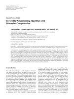
Figure 2: The channel estimation for colored input.
6. FURTHER IMPROVEMENT

We showed in Section 5 that the performance of our pro-
posed blind channel equalizer will converge asymptotically
to the MMSE equalizer as σ
2
n
→ 0. However, for low SNR,
the proposed algorithm will perform poorly due to the rough
approximation used in (39). There are methods available
to improve the SNR of the autocorrelation matrix. One is
the matrix denoising method introduced by Moulines et al.
[5]; another is the power of R (POR) method developed
by Xu et al. [14, 22]. Here, we borrow these ideas and
propose several extensions to our method that improve its
performance in the low SNR situation without performance
analyses. Application of each of these methods will only alter
Step 2 in our proposed algorithm, that is, the calculation of
matrix A. Instead of calculating A using T(γ
ext
)
H
R
−1
x
T(γ
ext
),
we provide three alternative methods to calculate A in this
case as follows.
(1) Matrix denoising method
A

= T

γ
ext

H

R
x
−

λ
min
− δ

I

−1
T

γ
ext

, (45)
where λ
min
is the minimum eigenvalue of R
x
and δ is a small
positive constant. This method is a straightforward extension

of the matrix denoising method in [5].
(2) POR method
A
= T

γ
ext

H
R
−m
x
T

γ
ext

, (46)
where m is a constant integer and m
≥ 1. Note that although
this POR method applies the same principle as the method
in both [14, 22], this POR method is different from that POR
method. As for the TX’s CMOV algorithm, the POR method
in [14] will not work for a channel with colored inputs.
25242322212019181716
SNR (dB)
0.01
0.015
0.02
0.025

0.03
0.035
0.04
0.045
0.05
0.055
0.06
NRMSE
TX’s CMOV algorithm
Proposed algorithm
Figure 3: SNR and channel estimation NRMSE for colored inputs.
(3) Hybrid method
Combine the denoising and the POR methods so that the
matrix A can be calculated using
A
= T

γ
ext

H

R
x
−

λ
min
− δ


I

−m
T

γ
ext

. (47)
We can see that these improvements are achieved at the cost
of increasing the computational complexity.
7. SIMULATIONS
We simulate an SIMO communication system as shown in
Figure 1. The FIR channel of order 15 is modeled by g(t)
=
c(t)−0.7c(t−T/3), where c(t) is a raised-cosine pulse limited
in 6T with roll-off factor 0.10 and with an oversampling
factor 3, that is, p
= 3inFigure 1.
7.1. Compare our method to previous CMOV methods
In this simulation, the input s(k) is generated by filtering
an .id 4-PAM signal with a causal FIR filter whose impulse
response coefficient vector is [
1
−0.30.14 0.12
]togen-
erate colored source. Please note, in practical application,
the colored sources may occur, for example, as a result
of channel encoding. We implement both our algorithm
and TX’s CMOV algorithm to equalize the linear channels.

In the implementation of our algorithm, we only use
the autocorrelation of the source, but not the FIR filter
coefficients. The order of the equalizers is 16. Figure 2 shows
the channel identification result at SNR
= 18 dB where the
number of delays is equal to 8 and the data length equals
6000. We find that both algorithms identify the channel
coefficients, though our method identifies the channel better
than does TX’s CMOV method in [13] because we make use
of the input statistics. In Figure 3, we show an average of 50
runs of the relationship between the SNR and the normalized
8 EURASIP Journal on Advances in Signal Processing
20151050
−0.5
0
0.5
1
(a)
20151050
−0.5
0
0.5
1
(b)
Figure 4: The overall response f (n) of the channel and equalizer
for colored input (a) based on TX’s CMOV algorithm, (b) Proposed
algorithm.
root mean-square error (NRMSE) of the estimated channel
parameters, which is defined as [11]:
NRMSE

=





1
Mq
Mq−1

n=0



h
capon
(n) − h(n)


2
. (48)
We notice that as the SNR decreases, the improvement of
our method over that of the TX CMOV algorithm is more
pronounced, as shown in Figure 3.InFigure 4, we show an
average of 50 runs of the overall response f (n)definedin
(17) at the SNR of 26 dB, from which we can see that our
algorithm successfully equalizes the channel distortion while
the TX’s CMOV method fails.
7.2. SER performance comparison
The previous simulations demonstrate that our proposed

algorithm can successfully equalize linear channels for both
colored and white inputs at relatively high SNR. The
superior performances of the L
´
opez-Valcarce algorithm [11]
over other blind linear channel equalization algorithms for
colored inputs, such as the subspace algorithm introduced
by Moulines et al. [5] and the algorithm introduced by
Afkhamie and Luo [12], have been demonstrated in [11]. As
a result, in this simulation, we only compare our proposed
algorithms with the L
´
opez-Valcarce algorithm [11]. As we
discussed earlier, the proposed algorithm performs poorly
at low SNR, so we also implement the improved algorithms
discussed in Section 6. In this simulation, the 3 linear
channels possess the same coefficients as before. The inputs
are the 4-QAM constellation, generated by the same rule as
in [11], that is,
s(n)
=
⎧
⎪
⎪
⎪
⎪
⎪
⎨
⎪
⎪

⎪
⎪
⎪
⎩
−
1+j if

b
n
b
n−1

=
(
00
)
+1 + j if

b
n
b
n−1

=
(
01
)
−1 − j if

b

n
b
n−1

=
(
10
)
+1 + j if

b
n
b
n−1

=
(
11
)
. (49)
16141210864
SNR (dB)
10
−4
10
−3
10
−2
10
−1

10
0
SER
1
2
3
4
5
Figure 5: SER comparison for different equalizers. (1) Proposed
algorithm without improvements discussed in Section 6,(2)L
´
opez-
Valcarce’s Method in [11] without denoising. (3) L
´
opez-Valcarce’s
method in [11] with matrix denoising. (4) Improved proposed
algorithm by the POR (m
= 3) method, (5) Improved proposed
method by the hybrid (m
= 2) method.
The {b
n
} is the input stream of iid bits, that is, b
n
∈{1,0}.
The order of all equalizers is 12, and the number of delays
equals 5. Figure 5 shows the average curve of 20 runs for
the relationship between the SNR and the symbol error rate
(SER) relationship of the L
´

opez-Valcarce algorithm and our
proposed algorithms.
From Figure 5, we can see that without the improvement
techniques discussed in Section 6 our proposed algorithm
does not generate satisfactory equalization. Nevertheless,
our improved algorithms based on the POR (with m
=
3) method and the hybrid (with m = 2) methods
outperform the L
´
opez-Valcarce algorithm and even the
L
´
opez-Valcarce algorithm with denoised autocorrelation
estimation. However, the L
´
opez-Valcarce algorithm with
autocorrelation matrix denoising usually requires three
singular value decompositions (SVD) of matrixes with size
of Mp
× Mp. To the contrary, our proposed algorithm
with POR improvement only requires one SVD to find the
minimum eigenvector. Furthermore, based on our proposed
new constraints, an adaptive blind channel equalization
method for a linear channel with colored input can be
straightforwardly developed using the same approach in
[15]. Consequently, we believe that our proposed algorithm
combined with the POR technique provides an excellent
solution for blind equalization of a linear channel with
colored input in term of performance and computational

complexity. We also conducted the same simulation but on
randomly generated channels, which generate the similar
relationship.
Yunhua Wang et al. 9
8. CONCLUSIONS
A new direct blind linear system equalization method has
been developed based on the constrained optimum method.
The resulting algorithm extracts channel information from
the noise subspace. However, unlike the previous TX’s
CMOV, our proposed algorithm is guaranteed to work for
either white or colored inputs with performance close to
that of the MMSE equalizer with high SNR input. The new
algorithm can be regarded as an extension of the CMOV
algorithm developed by Tsatsanis and Xu. Several methods
are introduced to improve the performance of the introduced
algorithm. Simulation results confirm the effectiveness of our
developed algorithms and analyses.
REFERENCES
[1] Z.DingandL.Ye,Blind Equalization and Identification,Marcel
Dekker, New York, NY, USA, 2001.
[2] K. Abed-Meraim, W. Qiu, and Y. Hua, “Blind system identifi-
cation,” Proceedings of the IEEE, vol. 85, no. 8, pp. 1310–1322,
1997.
[3] L. Tong, G. Xu, and T. Kailath, “Blind identification and
equalization based on second-order statistics: a time domain
approach,” IEEE Transactions on Information Theory, vol. 40,
no. 2, pp. 340–349, 1994.
[4] H. Liu, G. Xu, and L. Tong, “A deterministic approach to blind
identification of multi-channel FIR systems,” in Proceedings
of IEEE International Conference on Acoustics, Speech, and

Signal Processing (ICASSP ’94), vol. 4, pp. 581–584, Adelaide,
Australia, April 1994.
[5] E. Moulines, P. Duhamel, J F. Cardoso, and S. Mayrargue,
“Subspace methods for the blind identification of multichan-
nel FIR filters,” IEEE Transactions on Signal Processing, vol. 43,
no. 2, pp. 516–525, 1995.
[6] K. Abed Meraim, P. Duhamel, D. Gesbert, et al., “Predic-
tion error methods for time-domain blind identification of
multichannel FIR filters,” in Proceedings of the 20th IEEE
International Conference on Acoustics, Speech, and Signal
Processing (ICASSP ’95), vol. 3, pp. 1968–1971, Detroit, Mich,
USA, May 1995.
[7] D. T. M. Slock, “Blind fractionally-spaced equalization,
perfect-reconstruction filter banks and multichannel linear
prediction,” in Proceedings of IEEE International Conference on
Acoustics, Speech, and Signal Processing (ICASSP ’94), vol. 4,
pp. 585–588, Adelaide, Australia, April 1994.
[8] Q. Zhao and L. Tong, “Adaptive blind channel estimation
by least squares smoothing,” IEEE Transactions on Signal
Processing, vol. 47, no. 11, pp. 3000–3012, 1999.
[9] Z. Ding, “Blind channel identification algorithm based on
matrix outer-product,” in Proceedings of IEEE International
Conference on Communications (ICC ’96), vol. 2, pp. 852–856,
Dallas, Tex, USA, June 1996.
[10] Z. Ding, “Matrix outer-product decomposition method for
blind multiple channel identification,” IEEE Transactions on
Signal Processing, vol. 45, no. 12, pp. 3053–3061, 1997.
[11] R. L
´
opez-Valcarce and S. Dasgupta, “Blind channel equaliza-

tion with colored sources based on second-order statistics:
a linear prediction approach,” IEEE Transactions on Signal
Processing, vol. 49, no. 9, pp. 2050–2059, 2001.
[12] K. H. Afkhamie and Z Q. Luo, “Blind identification of
FIR systems driven by Markov-like input signals,” IEEE
Transactions on Signal Processing, vol. 48, no. 6, pp. 1726–1736,
2000.
[13] M. K. Tsatsanis and Z. Xu, “Constrained optimization meth-
ods for direct blind equalization,” IEEE Journal on Selected
Areas in Communications, vol. 17, no. 3, pp. 424–433, 1999.
[14] Z. Xu, P. Liu, and X. Wang, “Towards closing the gap between
MOE and subspace methods,” in Proceedings of the 36th
Asilomar Conference on Sig nals Systems and Computers, vol. 1,
pp. 689–693, Pacific Groove, Calif, USA, November 2002.
[15] Z. D. Xu and M. K. Tsatsanis, “Adaptive minimum variance
methods for direct blind multichannel equalization,” Signal
Processing, vol. 73, no. 1-2, pp. 125–138, 1999.
[16] J. Mannerkoski and V. Koivunen, “Autocorrelation properties
of channel encoded sequences-applicability to blind equaliza-
tion,” IEEE Transactions on Signal Processing, vol. 48, no. 12,
pp. 3501–3507, 2000.
[17] D. Zhou and V. DeBrunner, “Blind channel equalization with
colored source based on constrained optimization methods,”
in Proceedings of IEEE Global Telecommunications Conference
(GLOBECOM ’04), vol. 4, pp. 2286–2291, Dallas, Tex, USA,
November-December 2004.
[18] S. Haykin, Adaptive Filter Theory
, Prentice Hall, Upper Saddle
River, NJ, USA, 4th edition, 2004.
[19] J. Capon, “High-resolution frequency-wavenumber spectrum

analysis,” Proceedings of the IEEE, vol. 57, no. 8, pp. 1408–1418,
1969.
[20] L. Ljung, System Identification, Prentice Hall, Upper Saddle
River, NJ, USA, 2nd edition, 2002.
[21] D. H. Johnson and D. E. Dudgeon, Array Signal Processing:
Concepts and Techniques, Prentice-Hall, Englewood Cliffs, NJ,
USA, 1993.
[22] Z. Xu, P. Liu, and X. Wang, “Blind multiuser detection:
from MOE to subspace methods,” IEEE Transactions on Signal
Processing, vol. 52, no. 2, pp. 510–524, 2004.