Báo cáo hóa học: " Research Article A POMDP Framework for Coordinated Guidance of Autonomous UAVs for Multitarget Tracking" doc

Hindawi Publishing Corporation
EURASIP Journal on Advances in Signal Processing
Volume 2009, Article ID 724597, 17 pages
doi:10.1155/2009/724597
Research Article
A POMDP Framework for Coordinated Guidance of
Autonomous UAVs for Multitarget Tracking
Scott A. Miller,
1
Zachary A. Harris,
1
and Edwin K. P. Chong
2
1
Numerica Corporation, 4850 Hahns Peak Drive, Suite 200, Loveland, CO 80538, USA
2
Department of Electrical and Computer Engineering (ECE), Colorado State University, Fort Collins,
CO 80523-1373, USA
Correspondence should be addressed to Scott A. Miller,
Received 1 August 2008; Accepted 1 December 2008
Recommended by Matthijs Spaan
This paper discusses the application of the theory of partially observable Markov decision processes (POMDPs) to the design of
guidance algorithms for controlling the motion of unmanned aerial vehicles (UAVs) with onboard sensors to improve tracking
of multiple ground targets. While POMDP problems are intractable to solve exactly, principled approximation methods can
be devised based on the theory that characterizes optimal solutions. A new approximation method called nominal belief-state
optimization (NBO), combined with other application-specific approximations and techniques within the POMDP framework,
produces a practical design that coordinates the UAVs to achieve good long-term mean-squared-error tracking performance in the
presence of occlusions and dynamic constraints. The flexibility of the design is demonstrated by extending the objective to reduce
the probability of a track swap in ambiguous situations.
Copyright © 2009 Scott A. Miller et al. This is an open access article distributed under the Creative Commons Attribution License,
which permits unrestricted use, distribution, and reproduction in any medium, provided the original work is properly cited.

1. Introduction
Interest in unmanned aerial vehicles (UAVs) for applications
such as surveillance, search, and target tracking has increased
in recent years, owing to significant progress in their
development and a number of recognized advantages in their
use [1, 2]. Of particular interest to this special issue is the
interplay among signal processing, robotics, and automatic
control in the success of UAV systems.
This paper describes a principled framework for design-
ing a planning and coordination algorithm to control a
fleet of UAVs for the purpose of tracking ground targets.
The algorithm runs on a central fusion node that collects
measurements generated by sensors onboard the UAVs,
constructs tracks from those measurements, plans the future
motion of the UAVs to maximize tracking performance,
and sends motion commands back to the UAVs based on
the plan.
The focus of this paper is to illustrate a design framework
based on the theory of part ially obser vable Markov decision
processes (POMDPs), and to discuss practical issues related
to the use of the framework. With this in mind, the
problem scenarios presented here are idealized, and are
meant to illustrate qualitative behavior of a guidance system
design. Moreover, the particular approximations employed
in the design are examples and can certainly be improved.
Nevertheless, the intent is to present a design approach
that is flexible enough to admit refinements to models,
objectives, and approximation methods without damaging
the underlying structure of the framework.
Section 2 describes the nature of the UAV guidance

problem addressed here in more detail, and places it in
the context of the sensor resource management literature.
The detailed problem specification is presented in Section 3,
and our method for approximating the solution is dis-
cussed in Section 4. Several features of our approach are
already apparent in the case of a single UAV, as discussed
in Section 5. The method is extended to multiple UAVs
in Section 6, where coordination of multiple sensors is
demonstrated. In Section 7, we illustrate the flexibility of
the POMDP framework by modifying it to include more
complex tracking objectives such as preventing track swaps.
Finally, we conclude in Section 8 with summary remarks and
future directions.
2 EURASIP Journal on Advances in Signal Processing
2. Problem Description
The class of problems we pose in this paper is a rather
schematic representation of the UAV guidance problem.
Simplifications are assumed for ease of presentation and
understanding of the key issues involved in sensor coordi-
nation. These simplifications include the following.
2-D Motion. The targets are assumed to move in a plane on
the ground, while the UAVs are assumed to fly at a constant
altitude above the ground.
Position Measurements. The measurements generated by the
sensors are 2-D position measurements with associated
covariances describing the position uncertainty. A simplified
visual sensor (camera plus image processing) is assumed,
which implies that the angular resolution is much better than
the range resolution.
Perfect T racker. We assume that there are no false alarms

and no missed detections, so exactly one measurement is
generated for each target visible to the sensor. Also, perfect
data association is usually assumed, so the tracker knows
which measurement came from which target, though this
assumption is relaxed in Section 7 when track ambiguity is
considered.
Nevertheless, the problem class has a number of impor-
tant features that influence the design of a good planning
algorithm. These include the following.
Dynamic Constraints. These appear in the form of con-
straints on the motion of the UAVs. Specifically, the UAVs
fly at a constant speed and have bounded lateral acceleration
in the plane, which limits their turning radius. This is a
reasonable model of the characteristics of small fixed-wing
aircraft. The presence of dynamic constraints implies that the
planning algorithm needs to include some form of lookahead
for good long-term performance.
Randomness. Themeasurementshaverandomerrors,and
the models of target motion are random as well. However,
in most of our simulations the actual target motion is not
random.
Spatially Varying Measurement Error. The range error of the
sensor is an affine function of the distance between the sensor
and the target. The bearing error of the sensor is constant,
but that translates to a proportional error in Cartesian space
as well. This spatially varying error is what makes the sensor
placement problem meaningful.
Occlusions. There are occlusions in the plane that block the
visibility of targets from sensors when they are on opposite
sides of an occlusion. The occlusions are generally collections

of rectangles in our models, though in the case studies
presented they appear more as walls (thin rectangles). Targets
are allowed to cross occlusions, and of course the UAVs are
allowed to fly over them; their purpose is only to make the
observation of targets more challenging.
Tracking Objectives. The performance objectives considered
here are related to maintaining the best tracks on the targets.
Normally, that means minimizing the mean-squared error
between tracks and targets, but in Section 7 we also consider
the avoidance of track swaps as a performance objective.
This differs from most of the guidance literature, where the
objective is usually posed as interpolation of way-points.
In Section 3 we demonstrate that the UAV guidance
problem described here is a POMDP. One implication is
that the exact problem is in general formally undecidable
[3], so one must resort to approximations. However, another
implication is that the optimal solution to this problem is
characterized by a form of Bellman’s principle, and this prin-
ciple can be used as a basis for a structured approximation of
the optimal solution. In fact, the main goal of this paper is
to demonstrate that the design of the UAV guidance system
can be made practical by a limited and precisely understood
use of heuristics to approximate the ideal solution. That is,
the heuristics are used in such a way that their influence may
be relaxed and the solution improved as more computational
resources become available.
The UAV guidance problem considered here falls within
the class of problems known as sensor resource management
[4]. In its full generality, sensor resource management
encompasses a large body of problems arising from the

increasing variety and complexity of sensor systems, includ-
ing dynamic tasking of sensors, dynamic sensor place-
ment, control of sensing modalities (such as waveforms),
communication resource allocation, and task scheduling
within a sensor [5]. A number of approaches have been
proposed to address the design of algorithms for sensor
resource management, which can be broadly divided into
two categories: myopic and nonmyopic.
Myopic approaches do not explicitly account for the
future effects of sensor resource management decisions (i.e.,
there is no explicit planning or “lookahead”). One approach
within this category is based on fuzzy logic and expert
systems [6], which exploits operator knowledge to design
a resource manager. Another approach uses information-
theoretic measures as a basis for sensor resource manage-
ment [7–9]. In this approach, sensor controls are determined
based on maximizing a measure of “information.”
Nonmyopic approaches to sensor resource management
have gained increasing interest because of the need to
account for the kinds of requirements described in this
paper, which imply that foresight and planning are crucial
for good long-term performance. In the context of UAV
coordination and control, such approaches include the use
of guidance rules [2, 10–12], oscillator models [13], and
information-driven coordination [1, 14]. A more general
approach to dealing with nonmyopic resource management
involves stochastic dynamic programming formulations of
the problem (or, more specifically, POMDPs). As pointed out
in Section 4, exact optimal solutions are practically infeasible
to compute. Therefore, recent effort has focused on obtaining

EURASIP Journal on Advances in Signal Processing 3
approximate solutions, and a number of methods have
been developed (e.g., see [15–20]). This paper contributes
to the further development of this thrust by introducing
a new approximation method, called nominal belief-state
optimization, and applying it to the UAV guidance problem.
Approximation methods for POMDPs have been promi-
nent in the recent literature on artificial intelligence (AI),
under the rubric of probabilistic robotics [21]. In contrast
to much of the POMDP methods in the AI literature, a
unique feature of our current approach is that the state and
action spaces in our UAV guidance problem formulation is
continuous. We should note that some recent AI efforts have
also treated the continuous case (e.g., see [22–24]), though
in different settings.
3. POMDP Specification and Solution
In this section, we describe the mathematical formulation
of our guidance problem as a partially observable Markov
decision process (POMDP). We first provide a general
definition of POMDPs. We provide this background expo-
sition for the sake of completeness—readers who already
have this background can skip this subsection. Then, we
proceed to the specification of the POMDP for the guidance
problem. Finally, we discuss the nature of POMDP solutions,
leading up to a discussion of approximation methods in the
next section. For a full treatment of POMDPs and related
background, see [25]. For a discussion of POMDPs in sensor
management, see [5].
3.1. Definition of POMDP. A POMDP is a controlled dynam-
ical process, useful in modeling a wide range of resource

control problems. To specify a POMDP model, we need to
specify the following components:
(i) a set of states (the state space) and a distribution
specifying the random initial state;
(ii) a set of possible actions;
(iii) a state-transition law specifying the next-state distri-
butiongivenanactiontakenatacurrentstate;
(iv) a set of possible observations;
(v) an observation law specifying the distribution of
observations depending on the current state and
possibly the action;
(vi) a cost function specifying the cost (real number) of
being in a given state and taking a given action.
In the next subsection, we specify these components for our
guidance problem.
AsaPOMDPevolvesovertimeasadynamicalprocess,
we do not have direct access to the states. Instead, all we have
are the observations generated over time, providing us with
clues of the actual underlying states (hence the term partially
observable). These observations might, in some cases, allow
us to infer exactly what states actually occurred. However, in
general, there will be some uncertainty in our knowledge of
the states. This uncertainty is represented by the belief state,
whichisthea posteriori distribution of the underlying state
given the history of observations. The belief states summarize
the “feedback” information that is needed for controlling the
system. Conveniently, the belief state can easily be tracked
over time using Bayesian methods. Indeed, as pointed out
below, in our guidance problem the belief state is a quantity
that is already available (approximately) as track states.

Once we have specified the above components of a
POMDP, the guidance problem is posed as an optimization
problem where the expected cumulative cost over a time
horizon is the objective function to be minimized. The
decision variables in this optimization problem are the
actions to be applied over the planning horizon. However,
because of the stochastic nature of the problem, the optimal
actions are not fixed but are allowed to depend on the
particular realization of the random variables observed in
the past. Hence, the optimal solution is a feedback-control
rule, usually called a policy. More formally, a policy is
a mapping that, at each time, takes the belief state and
gives us a particular control action, chosen from the set of
possible actions. What we seek is an optimal policy. We will
characterize optimal policies in a later subsection, after we
discuss the POMDP formulation of the guidance problem.
3.2. POMDP Formulation of Guidance Problem. To f o r m u l a t e
our guidance problem in the POMDP framework, we must
specify each of the above components as they relate to
the guidance system. This subsection is devoted to this
specification.
States. In the guidance problem, three subsystems must be
accounted for in specifying the state of the system: the
sensor(s), the target(s), and the tracker. More precisely, the
state at time k is given by x
k
= (s
k
, ζ
k

, ξ
k
, P
k
), where s
k
represents the sensor state, ζ
k
represents the target state,
and (ξ
k
, P
k
) represents the track state. The sensor state s
k
specifies the locations and velocities of the sensors (UAVs) at
time k. The target state ζ
k
specifies the locations, velocities,
and accelerations of the targets at time k. Finally, the track
state (ξ
k
, P
k
) represents the state of the tracking algorithm;
ξ
k
is the posterior mean vector and P
k
is the posterior

covariance matrix, standard in Kalman filtering algorithms.
The representation of the state into a vector of state variables
is an instance of a factored model [26].
Action. In our guidance problem, we assume a standard
model where each UAV flies at constant speed and its motion
is controlled through turning controls that specify lateral
instantaneous accelerations. The lateral accelerations can
take values in an interval [
−a
max
, a
max
], where a
max
repre-
sents a maximum limit on the possible lateral acceleration.
So, the action at time k is given by a
k
∈ [−1, 1]
N
sens
,where
N
sens
is the number of UAVs, and the components of the
vector a
k
specify the normalized lateral acceleration of each
UAV.
State-Transition Law. The state-transition law specifies how

each component of the state changes from one-time step to
4 EURASIP Journal on Advances in Signal Processing
the next. In general, the transition law takes the following
form:
x
k+1
∼ p
k
(·|x
k
)(1)
for some time-varying distribution p
k
. However, the model
for the UAV guidance problem constrains the form of the
state transition law. The sensor state evolves according to
s
k+1
= ψ(s
k
, a
k
), (2)
where ψ is the map that defines how the state changes from
one-time step to the next depending on the acceleration
control as described above. The target state evolves according
to
ζ
k+1
= f (ζ

k
)+v
k
,(3)
where v
k
represents an i.i.d. random sequence and f
represents the target motion model. Most of our simulation
results use a nearly constant velocity (NCV) target motion
model, except for Section 6.2 which uses a nearly constant
acceleration (NCA) model. In all cases f is linear, and v
k
is
normally distributed. We write v
k
∼N (0, Q
k
) to indicate the
noise is normal with zero mean and covariance Q
k
.
Finally, the track state (ξ
k
, P
k
) evolves according to a
tracking algorithm, which is defined by a data association
method and the Kalman filter update equations. Since our
focus is on UAV guidance and not on practical tracking
issues, in most cases a “truth tracker” is used, which always

associates a measurement with the track corresponding to
the target being detected. Only in Section 7 is a nonideal
data association considered, for the purpose of evaluating
performance with ambiguous associations.
Observations and Observation Law. In general, the observa-
tion law takes the following form:
z
k
∼q
k
(·|x
k
)(4)
for some time-varying distribution q
k
. In our guidance
problem, since the state has four separate components, it is
convenient to express the observation with four correspond-
ing components (a factored representation). The sensor state
and track state are assumed to be fully observable. So, for
these components of the state, the observations are equal to
the underlying state components:
z
s
k
= s
k
, z
ξ
k

= ξ
k
, z
P
k
= P
k
. (5)
The target state, however, is not directly observable; instead,
what we have are random measurements of the target state
that are functions of the locations of the targets and the
sensors.
Let ζ
pos
k
and s
pos
k
represent the position vectors of the
target and sensor, respectively, and let h(ζ
k
, s
k
)beaboolean-
valued function that is true if the line of sight from s
pos
k
to
ζ
pos

k
is unobscured by any occlusions. Furthermore, we define
a 2D position covariance matrix R
k
(ζ
k
, s
k
) that reflects a 10%
uncertainty in the range from sensor to target, and 0.01π
radian angular uncertainty, where the range is taken to be
at least 10 meters. Then, the measurement of the target state
at time k is given by
z
ζ
k
=
⎧
⎨
⎩
ζ
pos
k
+ w
k
,ifh(ζ
k
, s
k
) = true,

∅ (no measurement), if h(ζ
k
, s
k
) = false,
(6)
where w
k
represents an i.i.d. sequence of noise values dis-
tributed according to the normal distribution N (0, R
k
(ζ
k
,
s
k
)).
Cost Function. The cost function we most commonly use in
our guidance problem is the mean-squared tracking error,
defined by the following:
C(x
k
, a
k
) = E
v
k
,w
k+1



ζ
k+1
−ξ
k+1

2
| x
k
, a
k

. (7)
In Section 7.1, we describe a different cost function which we
use for detecting track ambiguity.
Belief State. Although not a part of the POMDP specifica-
tion, it is convenient at this point to define our notation for
the belief state for the guidance problem. The belief state at
time k is given by the following:
b
k
=

b
s
k
, b
ζ
k
, b

ξ
k
, b
P
k

,(8)
where
b
s
k
(s) = δ(s −s
k
),
b
ζ
k
updated with z
ζ
k
using Bayes theorem
b
ξ
k
(ξ) = δ(ξ −ξ
k
),
b
P
k

(P) = δ(P − P
k
).
(9)
Note that those components of the state that are directly
observable have delta functions representing their corre-
sponding belief-state components.
We have deliberately distinguished between the belief
state and the track state (the internal state of the tracker).
The reason for this distinction is so that the model is
general enough to accommodate a variety of tracking
algorithms, even those that are acknowledged to be severe
approximations of the actual belief state. For the purpose of
control, it is natural to use the internal state of the tracker
as one of the inputs to the controller (and it is intuitive that
the control performance would benefit from the use of this
information). Therefore, it is appropriate to incorporate the
track state into the the POMDP state space, even if this is not
prima facie obvious.
3.3. Optimal Policy. Given the POMDP formulation of our
problem, our goal is to select actions over time to minimize
the expected cumulative cost (we take expectation here
because the cumulative cost is a random variable, being a
function of the random evolution of x
k
). To be specific,
suppose we are interested in the expected cumulative cost
over a time horizon of length H: k
= 0, 1, , H − 1.
EURASIP Journal on Advances in Signal Processing 5

The problem is to minimize the cumulative cost over horizon
H, given by the following:
J
H
= E

H−1

k=0
C(x
k
, a
k
)

. (10)
The goal is to pick the actions so that the objective function
is minimized. In general, the action chosen at each time
should be allowed to depend on the entire history up to that
time (i.e., the action at time k is a random variable that is a
function of all observable quantities up to time k). However,
it turns out that if an optimal choice of such a sequence of
actions exists, then there is an optimal choice of actions that
depends only on “belief-state feedback.” In other words, it
suffices for the action at time k to depend only on the belief
state at time k,asalludedtobefore.
Let b
k
be the belief state at time k, which is a distribution
over states,

b
k
(x) = P
x
k
(x | z
0
, ,z
k
; a
0
, ,a
k−1
) (11)
updated incrementally using Bayes rule. The objective can be
written in terms of belief states
J
H
= E

H−1

k=0
c(b
k
, a
k
) | b
0


, c(b, a) =

C(x, a)b(x)dx,
(12)
where E[
·|b
o
] represents conditional expectation given b
0
.
Let B represent the set of possible belief states, and let A
represent the set of possible actions. So what we seek is, at
each time k, a mapping π
∗
k
: B → A such that if we perform
action a
k
= π
∗
k
(b
k
), then the resulting objective function is
minimized. This is the desired optimal policy.
The key result in POMDP theory is Bellman’s principle.
Let J
∗
H
(b

0
) be the optimal objective function value (over
horizon H)withb
0
as the initial belief state. Then, Bellman’s
principle states that
π
∗
0
(b
0
) = argmin
a

c(b
0
, a)+E

J
∗
H−1
(b
1
) | b
0
, a

(13)
is an optimal policy, where b
1

is the random next belief state
(with distribution depending on a), E[
·|b
0
, a] represents
conditional expectation (given b
0
and action a)withrespect
to the random next state b
1
,andJ
∗
H−1
(b
1
) is the optimal
cumulative cost over the time horizon 1, , H starting with
belief state b
1
.
Define the Q-value of taking action a at state b
0
as
follows:
Q
H
(b
0
, a) = c(b
0

, a)+E

J
∗
H−1
(b
1
) | b
0
, a

. (14)
Then, Bellman’s principle can be rewritten as follows:
π
∗
0
(b
0
) = argmin
a
Q
H
(b
0
, a), (15)
that is, the optimal action at belief state b
0
is the one with
smallest Q-value at that belief state. Thus, Bellman’s principle
instructs us to minimize a modified cost function (Q

H
) that
includes the term E[J
∗
H−1
] indicating the expected future
cost of an action; this term is called the expected cost-to-
go (ECTG). By minimizing the Q-value that includes the
ECTG, the resulting policy has a lookahead property that is
a common theme among POMDP solution approaches.
For the optimal action at the next belief state b
1
,we
would similarly define the Q-value
Q
H−1
(b
1
, a) = c(b
1
, a)+E

J
∗
H−2
(b
2
) | b
1
, a


, (16)
where b
2
is the random next belief state and J
∗
H−2
(b
2
)is
the optimal cumulative cost over the time horizon 2, , H
starting with belief state b
2
. Bellman’s principle then states
that the optimal action is given by the following:
π
∗
1
(b
1
) = argmin
a
Q
H−1
(b
1
, a). (17)
A common approach in online optimization-based con-
trol is to assume that the horizon is long enough that the
difference between Q

H
and Q
H−1
is negligible. This has two
implications: first, the time-varying optimal policy π
∗
k
may
be approximated by a stationary policy, denoted π
∗
; second,
the optimal policy is given by the following:
π
∗
(b) = argmin
a
Q
H
(b, a), (18)
where now the horizon is fixed at H regardless of the current
time k. This approach is called receding horizon control,
and is practically appealing because it provides lookahead
capability without the technical difficulty of infinite-horizon
control. Moreover, there is usually a practical limit to how
far models may be usefully predicted. Henceforth, we will
assume the horizon length is constant and drop it from our
notation.
In summary, we seek a policy π
∗
(b) that, for a given belief

state b, returns the action a that minimizes Q(b, a), which in
the receding-horizon case is
Q(b, a)
= c(b, a)+E[J
∗
(b

) | b, a], (19)
where b

is the (random) belief state after applying action a
at belief state b,andc(b, a) is the associated cost. The second
term in the Q-value is in general difficult to obtain, especially
because the belief-state space is large. For this reason,
approximation methods are necessary. In the next section, we
describe our algorithm for approximating argmin
a
Q(b, a).
We should re-emphasize here that the action space
in our UAV guidance problem is a hypercube, which is
a continuous space of possible actions. The optimization
involved in performing argmin
a
Q(b, a) therefore involves
a search algorithm over this hypercube. Our focus in this
paper is on a new method to approximate Q(b, a) and not
on how to minimize it. Therefore, in this paper we simply
use a generic search method to perform the minimization.
More specifically, in our simulation studies, we used Matlab’s
fmincon function. We should point out that in related work,

other authors have considered the problem of designing a
good search algorithm (e.g., [27]).
6 EURASIP Journal on Advances in Signal Processing
4. Approximation Method
There are two aspects of a general POMDP that make it
intractable to solve exactly. First, it is a stochastic control
problem, so the dynamics are properly understood as
constraints on distributions over the state space, which are
infinite dimensional in the case of a continuous state space as
in our tracking application. In practice, solution methods for
Markov decision processes employ some parametric repre-
sentation or nonparametric (i.e., Monte Carlo or “particle”)
representation of the distribution, to reduce the problem
to a finite-dimensional one. Intelligent choices of finite-
dimensional approximations are derived from Bellman’s
principle characterizing the optimal solution. POMDPs,
however, have the additional complication that the state
space itself is infinite dimensional, since it includes the belief
state which is a distribution; hence, the belief state must also
be approximated by some finite-dimensional representation.
In Section 4.1, we present a finite-dimensional approxima-
tion to the problem called nominal belief-state optimization
(NBO), which takes advantage of the particular structure of
the tracking objective in our application.
Secondly, in the interest of long-term performance, the
objective of a POMDP is often stated over an arbitrarily long
or infinite horizon. This difficulty is typically addressed by
truncating the horizon to a finite length, the effect of which
is discussed in Section 4.2.
Before proceeding to the detailed description of our NBO

approach, we first make two simplifying approximations that
follow from standard assumptions for tracking problems.
The first approximation, which follows from the assumption
of a correct tracking model and Gaussian statistics, is that
the belief-state component for the target can be expressed as
follows:
b
ζ
k
(ζ) = N (ζ −ξ
k
, P
k
), (20)
and can be updated using (extended) Kalman filtering.
We adopt this approximation for the remainder of this
paper. The second approximation, which follows from the
additional assumption of correct data association, is that the
cost function can be written as follows:
c(b
k
, a
k
) =

E
v
k
,w
k+1


ζ
k+1
−ξ
k+1

2
| s
k
, ζ, ξ
k
, a
k

b
ζ
k
(ζ)dζ
= Tr P
k+1
.
(21)
In Section 7, we study the impact of this approximation
in the context of tracking with data association ambiguity
(i.e., when we do not necessarily have the correct data
association), and consider a different cost function that
explicitly takes into account the data association ambiguity.
4.1. Nominal Belief-State Optimization (NBO). Anumberof
POMDP approximation methods have been studied in the
literature. It is instructive to review these methods briefly,

to provide some context for our NBO approach. These
methods either directly approximate the Q-value Q(b, a)
or indirectly approximate the Q-value by approximating
the cost-to-go J
∗
(b), and include heuristic expected ECTG
[28], parametric approximation [29, 30], policy rollout [31],
hindsight optimization [32, 33], and foresight optimization
(also called open-loop feedback control (OLFC)) [25]. The
following is a summary of these methods, exposing the
nature of each approximation (for a detailed discussion
of these methods applied to sensor resource management
problems, see [15]):
(i) heuristic ECTG:
Q(b, a)
≈ c(b, a)+γN(b, a), (22)
(ii) parametric approximation (e.g., Q-learning):
Q(b, a)
≈

Q(b, a, θ), (23)
(iii) policy rollout:
Q(b, a)
≈ c(b, a)+E

J
π
base
(b


) | b

, (24)
(iv) hindsight optimization:
J
∗
(b) ≈ E

min
(a
k
)
k

k
c(b
k
, a
k
) | b

, (25)
(v) foresight optimization (OLFC):
J
∗
(b) ≈ min
(a
k
)
k

E


k
c(b
k
, a
k
) | b,(a
k
)
k

. (26)
The notation (a
k
)
k
means the ordered list (a
0
, a
1
, ).
Typically, the expectations in the last three methods are
approximated using Monte Carlo methods.
The NBO approach may be summarized as follows:
J
∗
(b) ≈ min
(a

k
)
k

k
c(

b
k
, a
k
), (27)
where (

b
k
)
k
represents a nominal sequence of belief states.
Thus, it resembles both the hindsight and foresight opti-
mization approaches, but with the expectation approximated
by one sample. The reader will notice that hindsight and
foresight optimizations differ in the order in which the
expectation and minimization is taken. However, because
NBO involves only a single sample path (instead of an expec-
tation), NBO straddles this distinction between hindsight
and foresight optimization.
The central motivation behind NBO is computational
efficiency. If one cannot afford to simulate multiple samples
of the random noise sequences to estimate expectations, and

only one realization can be chosen, it is natural to choose the
“nominal” sequence (e.g., maximum likelihood or mean).
The nominal noise sequence leads to a nominal belief-state
sequence (

b
k
)
k
as a function of the chosen action sequence
(a
k
)
k
. Note that in NBO, as in foresight optimization, the
EURASIP Journal on Advances in Signal Processing 7
optimization is over a fixed sequence (a
k
)
k
rather than a
noise-dependent sequence or a policy.
There are two points worth emphasizing about the
NBO approach. First, the nominal belief-state sequence is
not fixed, as (27) might suggest; rather, the underlying
random variables are fixed at nominal values and the belief
states become deterministic functions of the chosen actions.
Second, the expectation implicit in the incremental cost
c(


b
k
, a
k
)(recall(7)and(12)) need not be approximated by
the “nominal” value. In fact, for the mean-squared-error cost
we use in the tracking application, the nominal value would
be 0. Instead, we use the fact that the expected cost can be
evaluated analytically by (21) under the previously stated
assumptions of correct tracking model, Gaussian statistics,
and correct data association.
Because NBO approximates the belief-state evolution but
not the cost evaluation, the method is suitable when the
primary effect of the randomness appears in the cost, not
in the state prediction. Thus, NBO should perform well
in our tracking application as long as the target motion is
reasonably predictable with the tracking model within the
chosen planning horizon.
The general procedure for using the NBO approximation
may be summarized as follows.
(1) Write the state dynamics as functions of zero-mean
noise. For example, borrowing from the notation of
Section 3.2:
x
k+1
= f (x
k
, a
k
)+v

k
, v
k
∼N (0, Q
k
),
z
k
= g(x
k
)+w
k
, w
k
∼N (0, R
k
).
(28)
(2) Define nominal belief-state sequence (

b
1
, ,

b
H−1
)
b
k+1
= Φ(b

k
, a
k
, v
k
, w
k+1
) =⇒

b
k+1
= Φ(

b
k
, a
k
,0,0),

b
0
= b
0
,
(29)
in the linear Gaussian case, this is the MAP estimate
of b
k
.
(3) Replace expectation over random future belief states

J
H
(b
0
) = E
b
1
, ,b
H

H

k=1
c(b
k
, a
k
)

, (30)
with the sample given by nominal belief state
sequence
J
H
(b
0
) ≈
H

k=1

c(

b
k
, a
k
). (31)
(4) Optimize over action sequence (a
0
, ,a
H−1
).
As pointed out before, because our focus here is to introduce
NBO as a new approximation method, the optimization in
the last step above is taken to be a generic optimization
problem that is solved using a generic method. In our
simulation studies, we used Matlab’s fmincon function.
In the specific case of tracking, recall that the belief
state b
ζ
k
corresponding to the target state ζ
k
is identified
with the track state (ξ
k
, P
k
) according to (20). Therefore, the
nominal belief state


b
ζ
k
evolves according to the nominal track
state trajectory (

ξ
k
,

P
k
) given by the (extended) Kalman filter
equations with an exactly zero noise sequence. This reduces
to the following:

b
ζ
k
(ζ) = N

ζ −

ξ
k
,

P
k


,

ξ
k+1
= F
k

ξ
k
,

P
k+1
=

F
k

P
k
F
T
k
+ Q
k

−1
+ H
T

k+1

R
k+1


ξ
k
, s
k

−1
H
k+1

−1
,
(32)
where the (linearized) target motion model is given by the
following:
ζ
k+1
= F
k
ζ
k
+ v
k
, v
k

∼N (0, Q
k
),
z
k
= H
k
ζ
k
+ w
k
, w
k
∼N

0, R
k
(ζ
k
, s
k
)

.
(33)
The incremental cost given by the nominal belief state is then
c(

b
k

, a
k
) = Tr

P
k+1
=
N
targ

i=1
Tr

P
i
k+1
, (34)
where N
targ
is the number of targets.
4.2. Finite Horizon. In the guidance problem we are inter-
ested in long-term tracking performance. For the sake of
exposition, if we idealize this problem as an infinite-horizon
POMDP (ignoring the attendant technical complications),
Bellman’s principle can be stated as follows:
J
∗
∞
(b
0

) = min
π
E

H−1

k=0
c

b
k
, π(b
k
)

+ J
∗
∞
(b
H
)

(35)
for any H<
∞.ThetermE[J
∗
∞
(b
H
)] is the ECTG from the

end of the horizon H.IfH represents the practical limit of
horizon length, then (35) may be approximated in two ways:
J
∗
∞
(b
0
) ≈ min
π
E

H−1

k=0
c

b
k
, π(b
k
)


(truncation),
J
∗
∞
(b
0
) ≈ min

π
E

H−1

k=0
c

b
k
, π(b
k
)

+

J(b
H
)

(HECTG).
(36)
The first amounts to ignoring the ECTG term, and is often
the approach taken in the literature. The second replaces
the exact ECTG with a heuristic approximation, typically a
gross approximation that is quick to compute. To benefit
from the inclusion of a heuristic ECTG (HECTG) term in
the cost function for optimization,

Jneeds only to be a better

estimate of J
∗
∞
than a constant. Moreover, the utility of the
approximation is in how well it rank actions, not in how well
it estimates the ECTG. Section 5.4 will illustrate the crucial
role this term can play in generating a good action policy.
8 EURASIP Journal on Advances in Signal Processing
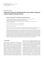
Figure 1: No occlusion with H = 1.
5. Single UAV Case
We begin our assessment of the performance of a POMDP-
based design with the simple case of a single UAV and two
targets, where the two targets move along parallel straight-
line paths. This is enough to demonstrate the qualitative
behavior of the method. It turns out that a straightforward
but naive implementation of the POMDP approach leads
to performance problems, but these can be overcome by
employing an approximate ECTG term in the objective, and
a two-phase approach for the action search.
5.1. Scenario Trajectory Plots. First, we describe what is
depicted in the scenario trajectory plots that appear through-
out the remaining sections. See, for example, Figures 1 and
2. Target location at each measurement time is indicated
by a small red dot. The targets in most scenarios move in
straight horizontal lines from left to right at constant speed.
The track covariances are indicated by blue ellipses at each
measurement time; these are 1-sigma ellipses corresponding
to the position component of the covariances, centered at
the mean track position indicated by a black dot. (However,
this coloring scheme is modified in later sections in order to

better distinguish between closely spaced targets.)
The UAV trajectory is plotted as a thin black line, with
an arrow periodically. Large X’s appear on the tracks that are
synchronized with the arrows on the UAV trajectory, to give
a sense of relative positions at any time.
Finally, occlusions are indicated by thick light green lines.
When the line of sight from a sensor to a target intersects an
occlusion, that target is not visible from that sensor. This is
a crude model of buildings or walls that block the visibility
of certain areas of the ground from different perspectives.
It is not meant to be realistic, but serves to illustrate the
effect of occlusions on the performance of the UAV guidance
algorithm.
5.2. Results with No ECTG. Following the NBO procedure,
our first design for guiding the UAV optimizes the cost
function (31) within a receding horizon approach, issuing
only the command a
0
and reoptimizing at the next step. In
the simplest case, the policy is a myopic one: choose the
next action that minimizes the immediate cost at the next
step based on current state information. This is equivalent
to a receding horizon approach with H
= 1 and no ECTG
term. The behavior of this policy in a scenario with two
targets moving at constant velocity along parallel paths is
illustrated in Figure 1. For this scenario, the behavior with
H>1 (applying NBO) is not qualitatively different. The
UAV’s speed is greater than the targets’, so the UAV is forced
to loop or weave to reduce its average speed. Moreover, the

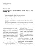
Figure 2: Gap occlusion with H = 1.
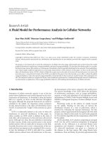
Figure 3: Gap occlusion with H = 4.
UAV tends to fly over one target than the other, instead of
staying in between. There are two main reasons for this. First,
the measurement noise is nonisotropic, so it is beneficial to
observe the targets from different angles over time. Second,
the trace objective is minimized by locating the UAV over the
target with the greater covariance trace.
To see this, consider a simplified one-dimensional
tracking problem with stationary targets on the real line
with positions x
1
and x
2
, sensor position y, and noisy
measurement of target positions given by
z
i
∼N

x
i
, ρ(y − x
i
)
2
+ r

, i = 1, 2. (37)
This noise model is analogous to the relative range uncer-

tainty defined in Section 3.2. If the current “track” variances
are given by p
1
and p
2
, then the variances after updating with
the Kalman filter, as a function of the new sensor location y,
are given by
p
+
i
(y) = (1 − k
i
)p
i
=
ρ(y −x
i
)
2
+ r
ρ(y − x
i
)
2
+ r + p
i
p
i
, i = 1, 2,

(38)
and the trace of the overall (diagonal) covariance is c(y)
=
p
+
1
(y)+p
+
2
(y). It is not hard to show that if the targets are
separated enough, c(y) has local minima at about y
= x
1
and y = x
2
with values of approximately p
2
+ p
1
r/(p
1
+r)and
p
1
+ p
2
r/(p
2
+ r), respectively. Therefore, the best location of
the sensor is at about x

1
if p
1
>p
2
, and at about x
2
if the
opposite is true.
Thus, the simple myopic policy behaves in a nearly
optimal manner when there are no occlusions. However,
if occlusions are introduced, some lookahead (e.g., longer
planning horizon) is necessary to anticipate the loss of
observations. Figure 2 illustrates what happens when the
planning horizon is too short. In this scenario, there are
two horizontal walls with a gap separating them. If the UAV
cannot cross the gap within the planning horizon, there is no
apparent benefit to moving away from the top target toward
the bottom target, and the track on the bottom target goes
stale. On the other hand, with H
= 4 the horizon is long
enough to realize the benefit of crossing the gap, and the
weaving behavior is recovered (see Figure 3).
EURASIP Journal on Advances in Signal Processing 9
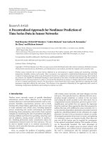
Figure 4: Gap occlusion with H = 4, search initialized with H = 1
plan.
In addition, to the length of the planning horizon,
another factor that can be important in practical perfor-
mance is the initialization of the search for the action
sequence. The result of the policy of initializing the four-

step action sequence with the output of the myopic plan
(H
= 1) is shown in Figure 4. The search fails to overcome
the poor performance of the myopic plan because the search
starts near a local minimum (recall that the trace objective
has local minima in the neighborhood of each target).
Bellman’s principle depends on finding the global minimum,
but our search is conducted with a gradient-based algorithm
(Matlab’s fmincon function), which is susceptible to local
minima. One remedy is to use a more reliable but expensive
global optimization algorithm. Another remedy, the one we
chose, is to use a more intelligent initialization for the search,
using a penalty term described in the next section.
5.3. Weighted Trace Penalty. The performance failures illus-
trated in the previous section are due to the lack of sensitivity
in our finite-horizon objective function (31) to the cost of
not observing a target. When the horizon is too short, it
seems futile to move toward an unobserved target if no
observations can be made within the horizon. Likewise, if the
action plan required to make an observation on an occluded
target deviates far enough from the initial plan, it may not
be found by a local search because locally there is no benefit
to moving toward the occluded target. To produce a solution
closer to the optimal infinite-horizon policy, the benefit of
initial actions that move the UAV closer to occluded targets
must be exposed somehow.
One way to expose that benefit is to augment the cost
function with a term that explicitly rewards actions that bring
the UAV closer to observing an occluded target. However,
such modifications must be used with caution. The danger

of simply optimizing a heuristically modified cost function
is that the heuristics may not apply well in all situations.
Bellman’s principle informs us of the proper mechanism
to include a term modeling a “hidden” long-term cost: the
ECTG term. Indeed, the blame for poor performance may
be placed on the use of truncation rather than HECTG as
the finite-horizon approximation to the infinite-horizon cost
(see Section 4.2).
In our tracking application, the hidden cost is the growth
of the covariance of the track on an occluded target while
it remains occluded. We estimate this growth by a weighted
trace penalty (WTP)term,whichisaproductofthecurrent
covariance trace and the minimum distance to observability
(MDO) for a currently occluded target, a term we define
precisely below. With the UAV moving at a constant speed,
Ta rg et
Sensor
D
p
MDO
Figure 5: Minimum distance to observability.
this is roughly equivalent to a scaling of the trace by the
time it takes to observe the target. When combined with the
trace term that is already in the cost function, this amounts
to an approximation of the track covariance at the time the
target is finally observed. More accurate approximations are
certainly possible, but this simple approximation is sufficient
to achieve the desired effect.
Specifically, the terminal cost or ECTG term using the
WTP has the following form:


J(b) = J
WTP
(b):= γD(s, ξ
i
)Tr P
i
, (39)
where γ is a positive constant, i is the index of the worst
occluded target
i
= argmax
i∈I
Tr P
i
,
I
={i | ξ
i
invisible from s},
(40)
and D(s, ξ) is the MDO, that is, the distance from the
sensor location given by s to the closest point p
MDO
(s, ξ)
from which the target location given by ξ is observable.
Figure 5 is a simple illustration of the MDO concept. Given
a single rectangular occlusion, p
MDO
(s, ξ)andD(s, ξ)can

be found very easily. Given multiple rectangular occlusions,
the exact MDO is cumbersome to compute, so we use a
fast approximation instead. For each rectangular occlusion
j,wecomputep
MDO
j
(s, ξ)andD
j
(s, ξ)asifj were the
only occlusion. Then we have D(s, ξ)
≥ max
j
D
j
(s, ξ) > 0
whenever ξ is occluded from s, so we use max
j
D
j
(s, ξ)asa
generally suitable approximation to D(s, ξ).
The reason a worst-case among the occluded targets is
selected, rather than including a term for each occluded
target, is that this forces the UAV to at least obtain an
observation on one target instead of being pulled toward two
separate targets and possibly never observing either one. The
true ECTG certainly includes costs for all occluded targets.
However, given that the ECTG can only be approximated, the
quality of the approximation is ultimately judged by whether
it leads to the correct ranking of action plans within the

horizon, and not by whether it closely models the true ECTG
value. We claim that by applying the penalty to only the worst
track covariance, the chosen actions are closer to the optimal
policy than what would result by applying the penalty to all
occluded tracks.
10 EURASIP Journal on Advances in Signal Processing
Figure 6: Behavior of WTP(1).
5.4. Results with WTP for ECTG. Let WTP(H) denote the
procedure of optimizing the NBO cost function with horizon
length H plus the WTP estimate of the ECTG:
min
a
0
, ,a
H−1
H−1

k=0
c(

b
k
, a
k
)+J
WTP
(

b
H

). (41)
Initially, we consider the use of WTP(1) in two different
roles: adapting the horizon length and initializing the action
search. Subsequently, we consider the effect of the terminal
cost in WTP(H)withH>1.
Figure 6 shows the behavior of WTP(1) on the gap
scenario previously considered, using a penalty weight of
just γ
= 10
−6
. Comparing with Figure 2, which has the same
horizon length but no penalty term, we see that the WTP
has the desired effect of forcing the UAV to alternately
visit each target. Therefore, the output of WTP(1) is a
reasonable starting point for predicting the trajectory arising
from a good action plan. Since WTP(1) is really a form
of Q-value approximation (namely, the heuristic ECTG
approach mentioned in the beginning of Section 4.1), it is
not surprising that it generates a nonmyopic policy that
outperforms the myopic policy, even though both policies
evaluate the incremental cost c at only one step.
By playing out a sequence of applications of WTP
(1)—which amounts to a sequence of one-dimensional
optimizations—we can quickly generate a prediction of
sensor motion that is useful for adapting the planning hori-
zon and initializing the multistep action search, potentially
mitigating the effects seen in Figures 2 and 4.Thus,weusea
three-step algorithm described as follows.
(1) Generate an initial action plan by a sequence of H
max

applications of WTP(1).
(2) Choose H to be the minimum number of steps such
that there is no change in observability of any of the
targets after that time, with a minimum value of H
min
.
(3) Search for the optimal H-step action sequence,
starting at the initial plan generated in step 1.
This can be considered a two-phase approach, with the first
two steps constituting Phase I and the third step being Phase
II. The heuristic role of WTP(1) in the above algorithm
is appropriate in the POMDP framework, because any
suboptimal behavior caused by the heuristic in Phase I has
a chance of being corrected by the optimization over the
longer horizon in Phase II, provided H
min
and H
max
are large
enough. Figure 7 shows the effectiveness of using WTP(1) to
choose H and initialize the search. In this test, H
min
= 1and
H
max
= 8, and the mean value of the adaptive H is 3.7, which
Figure 7: WTP(1) used for initialization and adaptive horizon.
Figure 8: Effect of truncated horizon with no ECTG.
Figure 9: Behavior of WTP(H) policy.
corresponds approximately to H = 4inFigure 3 but without

having to identify that value beforehand.
In practice, however, the horizon length is always
bounded above in order to limit the computation in
any planning iteration, and the upper bound H
max
may
sometimes be too small to achieve the desired performance.
Figure 8 illustrates such a scenario. There is only one
occlusion, but it is far enough from the upper target that
once the UAV moves sufficiently far from the occlusion, the
horizon is too short to realize the benefit of heading toward
the lower target when minimizing the trace objective. This
is despite the fact that the search is initialized with the UAV
headed straight down according to WTP(1).
The remedy, of course, is to use WTP as the ECTG in
Phase II, that is, to employ WTP(H)asin(41). The effect
of WTP(H) is depicted in Figure 9. In general, the inclusion
of the ECTG term makes lookahead more robust to poor
initialization and short horizons.
In general, we would not expect the optimal trajectory
to be symmetric with respect to the two targets, because of
a number of possible factors, including: (1) the location of
the occlusions, and (2) the dynamics and the acceleration
constraints on the UAV. In Figures 6 and 9, we see this
asymmetry in that the UAV does not spend equal amounts
of time near the two targets. In Figure 9, the position of the
occlusion is highly asymmetric in relation to the path of the
two targets—in this case, it is not surprising that the UAV
trajectory is also asymmetric. In Figure 6, the two occlusions
are more symmetric, and we would expect a more symmetric

trajectory in the long run. However, in the short run, the UAV
trajectory is not exactly symmetric because of the timing
and direction of the UAV as it crosses the occlusion. The
particular timing and direction of the UAV results in the need
for an extra loop in some instances but not others.
EURASIP Journal on Advances in Signal Processing 11
6. Multiple UAV Case
As it stands, the procedure developed for the single UAV case
is ill-suited to the case of multiple UAVs, because the WTP
is defined with only a single sensor in mind. An extension of
the WTP to multiple sensors is developed in Section 6.1,and
in Section 6.2 this extension is applied to a new scenario to
demonstrate the coordination of two sensors.
6.1. Extension of WTP. A slight modification of the WTP
defined in (39) can certainly be used as an ECTG in scenarios
with more than one sensor, for example:

J(b) = γ min
j
D(s
j
, ξ
i
)Tr P
i
, (42)
where s
j
is the state of sensor j. However, this underutilizes
the sensors, because only one sensor can affect the ECTG.

One would like the ECTG to guide two sensors toward two
separate occluded targets if it makes sense to do so. On the
other hand, if one sensor can “cover” two occluded targets
efficiently, there is no need to modify the motion of a second
sensor. The problem, therefore, is to decide which sensor will
receive responsibility for each occluded target.
It is natural to assign the “nearest” sensor to an occluded
target, that is, the one that minimizes the MDO as in (42).
However, to account for the effect of previous assignments
to that sensor, the MDO should not be measured along a
straight line directly from the starting position of the sensor,
but rather, along the path the sensor takes while making
observations on previously assigned targets. In the spirit of
the WTP for a single sensor, it is assumed that if multiple
occluded targets are assigned to a sensor, the most uncertain
track (the one with the highest covariance trace) is the one
that appears in the WTP and governs the motion of the
sensor, until the target is actually observed; then, the next
most uncertain track appears in the WTP, and so on. So,
roughly speaking, the sensor makes observations of occluded
targets in order of decreasing uncertainty.
Therefore, a multiple weighted trace penalty (MWTP)
term is computed according to the following procedure.
(1) Find the set of targets occluded from all sensors, and
sort in order of decreasing Tr P
i
.
(2) Set

J = 0, and D

j
= 0 for each sensor j.
(3) For each occluded target i (in order):
(a) find j
= argmin
j
{D
j
+ D(s
j
, ξ
i
)};
(b) if D
j
= 0 then set

J ←

J + γD(s
j
, ξ
i
)Tr P
i
;
(c) set D
j
← D
j

+ D(s
j
, ξ
i
)ands
j
← p
MDO
(s
j
, ξ
i
).
This procedure is an approximation in several respects. First,
it ignores the motion of the targets in the interval of time it
takes the sensor to move from one p
MDO
location to the next.
Second, it ignores the dynamic constraints of the UAVs. The
total distance is computed by a greedy, suboptimal algorithm.
None of these deficiencies is insurmountable, but for the
purpose of a quick heuristic ECTG for ranking action plans,
thisMWTPissufficient.
Figure 10: Beginning of scenario: sensors cover separate regions.
Figure 11: Transition: sensors coordinate plans to cover all targets
as one target moves.
6.2. Coordinated Sensor Motion. Figures 10, 11,and12
show snapshots of a scenario illustrating the coordination
capability of the guidance algorithm using the MWTP from
the previous section as an ECTG term. There are three

targets (red, blue, and black) and two sensor UAVs (black
and green). This scenario also demonstrates the adaptive
horizon, with thin magenta and orange lines showing the
UAVs’ planned Phase I and Phase II trajectories, respectively,
according to the current horizon length H.
Initially, the three targets are divided into two regions by
an occlusion, and one sensor covers each region. At this point
H
= 1isasufficient horizon. Then, the black target heads
down and crosses two occlusions to enter the bottom region.
In response, the green UAV chases after the downward-
bound target, while the black UAV moves to cover both upper
regions—the sensors coordinate to maximize coverage of the
targets. Figure 11 plots the UAV motion plans at the moment
the planner decides to chase the downward-bound target. A
large black X marks the spot from which the green sensor
expects to first see the black target. Generally speaking, the
longer the planning horizon, the earlier the UAVs react to the
downward-bound target, and the less time any target remains
unseen by a sensor. In the moment depicted in the figure,
12 EURASIP Journal on Advances in Signal Processing
Figure 12: End of scenario: sensors have coordinated for maximum
coverage.
Phase I has predicted that the black target is going to cross
the occlusion, and thus the adaptive horizon has increased to
H
= 6.
Unlike the previous scenarios, this scenario features
random target motion as well as random measurement noise.
This allows a broader comparison of performance among

different planning algorithms. Figure 13 shows a plot of the
empirical cumulative distribution function (CDF) of the
average tracking performance of seven algorithms: H
=
1 with no ECTG term, MWTP(1), MWTP(3), MWTP(4),
MWTP(5), MWTP(6), and MWTP(H) with adaptive H
between 1 and 6. The plot shows that the use of the
approximate ECTG produces substantially better perfor-
mance. Without the MWTP term in the objective, one of the
targets (usually the downward-bound one) is ignored when
it becomes occluded. There appears to be a minor benefit to
using H
= 1 or adaptive horizon over the other settings.
However, one should not make too much of this apparent
ranking. Perturbations of the problem configuration or other
parameters result in other performance rankings, though in
all cases MWTP significantly outperforms the pure myopic
policy lacking ECTG.
7. Track Ambiguity
Track accuracy metrics, such as the mean-squared-error
metric proposed in Section 3.2, are not the only measure
of tracking performance. Other considerations such as track
16001400120010008006004002000
Root mean squared track position error
Tr P, H
= 1
MWTP(1)
MWTP(3)
MWTP(4)
MWTP(5)

MWTP(6)
MWTP(H)
0
0.1
0.2
0.3
0.4
0.5
0.6
0.7
0.8
0.9
1
Cumulative frequency
Tr PMWTP
Two sensor, three target scenario; 3000 Monte Carlo runs
Figure 13: CDF of tracking performance in multi-sensor scenario.
duration and track continuity are also important. In partic-
ular, when target ID or threat class information is attached
to a track through some separate discrimination process, it
is important to maintain a consistent association between
the track and the target it represents. So-called “track
swaps” (switches in the mapping between targets and tracks)
may be caused by incorrect data association—updating a
track with measurements from a different target—or by
approximation of the true Bayesian update of the target state
distribution that the track state represents. The latter cause
is mainly a function of the tracking algorithm; the multiple
hypothesis tracking (MHT) algorithm with an unlimited
hypothesis set represents the true Bayesian update under

standard assumptions [34], but any practical tracker is an
approximation of the ideal. Data association ambiguity, on
the other hand, is a function of the sensor locations as
well as the tracker, and therefore minimizing this quantity
is a suitable objective in the UAV guidance problem. In
this section, we demonstrate the flexibility of the POMDP
framework by augmenting the mean-squared-error cost
function with a term that represents the risk of a track swap,
and applying the same basic algorithm to demonstrate how
the guidance algorithm reduces the probability of a track
swap in a scenario where the targets are confusable.
7.1. Detect ing Ambiguity. A challenge of this exercise is
thatitishardtopredicttrackswapswithNBO,since
the full spectrum of uncertainty is not explored. In the
context of predicting the performance of a proposed action
sequence, one could try to detect a track swap by comparing
associations of predicted track states and predicted target
states. This approach might work within a Monte Carlo
approximation method such as hindsight optimization, fore-
sight optimization, or policy rollout. With NBO, however,
EURASIP Journal on Advances in Signal Processing 13
the only predicted target state is the one that comes from
the maximum likelihood value of the predicted track state,
so the best data association will always be the “correct” one.
We must resort to a more indirect approach, measuring
a quantity that serves as a predictor of a likely track
swap.
The assessment of data association ambiguity is currently
a topic of concern in tracking [35], because of its role
as an indicator of the potential for error in track states

and track identity. Nevertheless, the ambiguity of a single
measurement-to-track data association is not a reliable
predictor of track swap. Consider the case of two targets
that cross each other at an oblique angle, which are tracked
with an NCV model updated with position measurements.
Despite the complete ambiguity of association at the point
when the targets cross, a track swap is extremely unlikely
under a reasonable track update rate because the velocity
estimate is unaffected by the ambiguity. Furthermore, tracks
can become confusable after accumulating a series of updates
with slightly ambiguous data associations, none of which is
egregious enough by itself to indicate trouble. This suggests
using an extended period of data association ambiguity as a
predictor of track swap; however, one can easily envision a
scenario in which one or two misassociations is enough to
cause a track swap.
Similarity of target state distributions (belief states)
should be a better indicator of the potential for a track swap.
If two tracks have similar distributions, it is unlikely that the
targets they represent can be reliably discriminated from each
other, now or in the future. For this approach to work, the
belief-state updates must reflect the inherent ambiguity of
the target states. It will not suffice to use a single-hypothesis
tracker in the prediction of belief states, even if the data
association is correct as it is in the “truth tracker” used
elsewhere in this paper. Again, a full MHT algorithm is
required to represent the true Bayesian update of the belief
states, which is intractable exactly when data association is
ambiguous. We have found that when the hypothesis set
is truncated to a reasonable limit, the MHT has trouble

representing uncertainty over extended periods of time.
Instead, we use the joint probability data association (JPDA)
algorithm [36] for belief-state (and track-state) updates in
this context, because it is designed to represent track state
uncertainty but in the compressed representation of one
Gaussian distribution per track.
The dissimilarity between distributions may be measured
in several ways: Kullback-Leibler divergence (or alpha diver-
gence), Bhattacharyya distance, or discordance [37], all of
which have closed-form solutions for Gaussians. However,
these measures are basically average-case measures of how
often the state values from the two distributions are within
a small neighborhood of each other. It turns out that a
worst-case metric is a better predictor of the potential for a
track swap. The reason for this is that track swaps are more
closely associated with instantaneous ambiguities in the track
associations. Specifically, even if on average the state variables
from two tracks are not often close, even a single occurrence
of an ambiguous measurement can cause a track swap. The
worst-case metric we use is defined next.
Given a Gaussian distribution N (μ, P), define the “χ
2
value” as follows:
χ
2
μ,P
(x):= (x −μ)
T
P
−1

(x −μ), (43)
so called because when x
∼N (μ, P) the quantity has an
χ
2
distribution with n degrees of freedom, where n is the
number of components in x. This is the square of the
Mahalanobis distance from μ to x. We define a worst-case
“χ
2
distance” between two Gaussian distributions N (μ
1
, P
1
)
and N (μ
2
, P
2
) as follows:
D
χ
2
(μ
1
, P
1
; μ
2
, P

2
)
:
= min

d |∃x  χ
2
μ
1
,P
1
(x) ≤ d, χ
2
μ
2
,P
2
(x) ≤ d

=
min
x
max

χ
2
μ
1
,P
1

(x), χ
2
μ
2
,P
2
(x)

.
(44)
Note that it makes sense to compare χ
2
μ
1
,P
1
(x)andχ
2
μ
2
,P
2
(x)
since they have the same distribution when x is drawn
randomly from N (μ
1
, P
1
)andN (μ
2

, P
2
), respectively. Geo-
metrically, D
χ
2
may be interpreted as the smallest d such
that the ellipsoid level surfaces χ
2
μ
1
,P
1
(x) = d and χ
2
μ
2
,P
2
(x) =
d just touch each other. Analytically, the problem may be
seen as measuring the distance between μ
1
and μ
2
but using
two different distance metrics. One way to use two different
metrics is to consider the set of points “equidistant” from
the two means, that is, the points having the same distance
from each mean using the applicable Mahalanobis distance

from each mean. Then, the desired distance is given by the
equidistant point with the least distance. Strictly speaking,
D
χ
2
(or its square root) is not a distance because it does not
satisfy the triangle inequality, but it does satisfy symmetry
and positivity, with a value of zero only when the means
agree.
The computation of D
χ
2
is a quasiconvex problem, which
can be solved with a bisection method involving a generalized
eigenvalue problem at each iteration, according to the S-
procedure [38]. This is a rather expensive procedure to
execute as part of a single objective function evaluation.
However, empirical tests revealed that one of the upper
bounds used in the bisection method tends to be a constant
factor of the true value in both ambiguous and unambiguous
situations, so we elected to use that as a surrogate for D
χ
2
.
The upper bound in question is obtained by restricting the
problem to the line segment between μ
1
and μ
2
:


D
χ
2
(μ
1
, P
1
; μ
2
, P
2
):= min
α∈[0,1]
max

χ
2
μ
1
,P
1
(μ
1
+ α(μ
2
−μ
1
)),
χ

2
μ
2
,P
2
(μ
1
+ α(μ
2
−μ
1
))

.
(45)
If a point y lies in two intervals along that line segment
starting at opposite ends, and y has the same χ
2
value d to
each mean, then surely the ellipsoidal sets given by χ
2
μ
1
,P
1
(x) ≤
d and χ
2
μ
2

,P
2
(x) ≤ d intersect because y is contained in
the intersection. Therefore, d is an upper bound on the
minimum distance such that there is an intersection, that
is,

D
χ
2
(μ
1
, P
1
; μ
2
, P
2
) ≥ D
χ
2
(μ
1
, P
1
; μ
2
, P
2
). The upper bound

is computed by simply solving a quadratic equation, which
14 EURASIP Journal on Advances in Signal Processing
Figure 14: Tr P objective in ambiguity scenario.
Figure 15: Tr P + γ/

D
χ
2
objective in ambiguity scenario.
determines the α ∈ [0,1] such that the two χ
2
values in (45)
are equal.
7.2. Benefits of Ambiguity Objective. Using the method from
Section 5, a sensor tracking two targets will try to stay near
to both targets, indeed between them if possible, thereby
minimizing ambiguity even without an explicit measure of
ambiguity in the objective function. Thus to demonstrate
the effect of a planner that deliberately seeks to minimize
ambiguity requires a scenario in which at least one sensor is
assigned to track at least three targets on its own.
The scenario depicted in Figures 14 and 15 demonstrates
a genuine tradeoff that has to be made by the planner. Two
of the targets (red and blue) are traveling very close to each
other. The third (black) target is far away from the other
two. If the sensor stays near the two bottom targets then it
has a good chance of maintaining a clear picture of which
is which, but its estimate of the top target’s state remains at
a consistently poor quality. If the sensor “weaves” between
the top and bottom targets then it can maintain a more

balanced level of estimated error amongst the targets, but it
is much more likely to confuse the identity of the bottom
two. Recall from Section 5.2 that weaving optimizes the mean
squared tracking error objective when tracking targets that
are distant from each other. With the same mean-squared-
error objective function (approximated by Tr P), the same
behavior occurs in this scenario (Figure 14)exceptmoretime
is spent in the lower region with the two closely spaced
targets. By adding a term proportional to 1/

D
χ
2
to the cost,
a penalty is placed on ambiguity of track states, and as seen
in Figure 15, the result is that the sensor stays near the two
bottom targets.
The outcomes shown in Figures 14 and 15 are in fact
representative of the behavior of the two different objective
functions over multiple Monte Carlo runs. Figure 16 plots
the cumulative distribution of the fraction of incorrect data
associations over the course of each of 5000 Monte Carlo
simulations. The weaving behavior produced by the trace
0.90.80.70.60.50.40.30.20.10
Percent of incorrect track to measurement associations
Tr P, H
= 1
Tr P, H
= 6
Tr P +γ/


D
χ
2
, H = 1
Tr P +γ/

D
χ
2
, H = 6
1/D
χ
2
, H = 1
0
0.1
0.2
0.3
0.4
0.5
0.6
0.7
0.8
0.9
1
Cumulative frequency
Tr P
One sensor, three target ambiguity scenario; 5000 Monte Carlo runs
Figure 16: CDF of data association error rate in ambiguity scenario.

Table 1: Frequency of correct track association at end of scenario.
Objective H %CorrectID
Tr P 1 70.14%
Tr P 6 58.58%
Tr P + γ/

D
χ
2
1 97.04%
Tr P + γ/

D
χ
2
6 97.02%
1/D
χ
2
1 97.20%
objective clearly results in a higher proportion of association
errors. However, as mentioned in Section 7.1, individual
track to measurement associations are not our concern per
se, but rather the correctness of the final track to truth
association after the targets separate. Tab le 1 summarizes
how frequently tracks are assigned to the correct target ID
at the end of the scenario. Again, the benefit of including
D
χ
2

or

D
χ
2
for ambiguity avoidance is clear. (Note that in the
presence of complete ambiguity between the two targets on
the bottom, we could guess the correct target ID by a coin
flip and expect 50% accuracy.)
While the above results demonstrate the success of our
ambiguity objective in accomplishing what it was explicitly
designed for, one additional positive outcome from this
scenario may be surprising at first. The objective functions
that include ambiguity tend to produce a better overall
mean-squared-tracking error than the trace objective alone,
as seen in Figure 17. The reason is the latter equality in
(21) assumes correct data association. In other words, in the
presence of ambiguity, the trace of the position covariance
no longer represents the mean-squared-track error relative
to truth. As such, we can view the term 1/D
χ
2
as a heuristic
ECTG—the term plays a similar role as the ECTG term
EURASIP Journal on Advances in Signal Processing 15
350300250200150100500
Root mean squared track position error
Tr P, H
= 1
Tr P, H

= 6
Tr P,+γ/

D
χ
2
, H = 1
Tr P +γ/

D
χ
2
, H = 6
1/D
χ
2
, H = 1
0
0.1
0.2
0.3
0.4
0.5
0.6
0.7
0.8
0.9
1
Cumulative frequency
Tr P

One sensor, three target ambiguity scenario; 5000 Monte Carlo runs
Figure 17: CDF of RMS track error in ambiguity scenario.
in Section 6 and contributes to improvement in the overall
tracking performance.
The histogram in Figure 18 shows a clear bimodal
distribution when using the trace objective, apparently
corresponding to the cases where a track swap does or
does not occur, respectively. Although the trace objective
produces good tracking performance when no track swap
occurs, the significant second mode leads to a poor average
performance result. In contrast, Figure 19 shows that when
the objective includes ambiguity, the mean-squared error
is heavily distributed around a single mode with a very
low weight on the second mode (even with the ambiguity
objective the sensor occasionally produces a track swap
because constraints on the UAV motion prohibit it from
remaining in place between the two targets).
8. Conclusion
Our main contribution in this paper is a demonstration
of the effectiveness of the POMDP formalism as basis for
designing a solution to a complex resource management
problem. The application of ideas from POMDP theory is
not straightforward because approximations must be made
in order to develop a practical solution. Nevertheless, by
grounding the design approach in the principles of POMDP,
we can preserve the key advantages of the theoretical
framework, namely the flexibility to handle complex models
and objectives, and the lookahead nature of the solution.
We have illustrated both of those advantages in the
UAV guidance examples presented here. These simplified

examples were designed to highlight some of the central
issues involved in the practical application of POMDP-
based design. They identified the benefit of a nonmyopic
policy, the crucial importance of an approximate ECTG
120100806040200
Root mean squared track position error
Tr P, H
= 1
0
100
200
300
400
500
600
700
Frequency
Figure 18: Histogram of RMS track error, Tr P objective, H = 1.
120100806040200
Root mean squared track position error
Tr P +γ/

D
χ
2
, H = 1
0
100
200
300

400
500
600
700
Frequency
Figure 19: Histogram of RMS track error, Tr P + γ/

D
χ
2
objective,
H
= 1.
term in the objective, the structured roles that heuristics can
play in the algorithm (e.g., adaptive horizon length, search
initialization), and the ability to change the objective without
major redesign.
We have also presented a new approximation method
called nominal belief-state optimization (NBO) which is
particularly well suited to the tracking application considered
here, because under standard assumptions the expected cost
can be computed analytically. As NBO is a special case of
hindsight optimization and foresight optimization, a design
based on NBO is easily extended to these more computation-
ally expensive methods if more accurate representation of the
randomness of the problem is required.
As our main goal in this paper is to illustrate some of
the practical issues involved in applying the POMDP-based
design approach, the actual guidance system developed here
16 EURASIP Journal on Advances in Signal Processing

is not meant to be taken as the best design we could achieve.
There are many directions in which the algorithm could be
improved, including:
(i) a more accurate MDO approximation;
(ii) a more global search for the optimal action plan;
(iii) an adaptive weight on the ECTG term (which
currently requires some tuning);
(iv) a different parameterization of the action space that
allows for longer planning horizons while limiting
the growth of the search space;
(v) a limited use of Monte Carlo methods to explore
alternative futures other than the nominal belief-state
sequence.
The conclusion we wish to emphasize is that the principled
framework of a POMDP-based design provides an under-
standing of where approximations are applied, leading to
avenues of performance improvement (such as the ones
listed above) as more computational resources become
available.
Acknowledgments
This work was supported by AFOSR Grant no. FA9550-07-
1-0360 and NSF Grant no. ECCS-0700559.
References
[1] B.Grocholsky,J.Keller,V.Kumar,andG.Pappas,“Coopera-
tive air and ground surveillance,” IEEE Robotics & Automation
Magazine, vol. 13, no. 3, pp. 16–26, 2006.
[2] R. A. Wise and R. T. Rysdyk, “UAV coordination for auton-
omous target tracking,” in Proceedings of the AIAA Guidance,
Navigation, and Control Conference, pp. 3210–3231, Keystone,
Colo, USA, August 2006.

[3] O. Madani, S. Hanks, and A. Condon, “On the undecid-
ability of probabilistic planning and infinite-horizon partially
observable Markov decision problems,” in Proceedings of the
16th National Conference on Artificial Intelligence (AAAI ’99),
pp. 541–548, Orlando, Fla, USA, July 1999.
[4] S. Musick, “Defense applications,” in Foundations and Appli-
cations of Sensor Management, A. O. Hero III, D. Casta
˜
non,
D. Cochran, and K. Kastella, Eds., chapter 11, Springer, New
York, NY, USA, 2007.
[5] A.O.HeroIII,D.Casta
˜
non, D. Cochran, and K. Kastella, Eds.,
Foundations and Applications of Sensor Management, Springer,
New York, NY, USA, 2008.
[6] S. Miranda, C. Baker, K. Woodbridge, and H. Griffiths,
“Knowledge-based resource management for multifunction
radar,” IEEE Signal Processing Magazine,vol.23,no.1,pp.66–
76, 2006.
[7] W. Schmaedeke and K. Kastella, “Information based sensor
management and IMMKF,” in Signal and Data Processing of
Small Targets, vol. 3373 of Proceedings of SPIE, pp. 390–401,
Orlando, Fla, USA, April 1998.
[8]B.P.Grocholsky,H.F.Durrant-Whyte,andP.W.Gibbens,
“Information-theoretic approach to decentralized control of
multiple autonomous flight vehicles,” in Sensor Fusion and
Decentralized Control in Robotic Systems III, vol. 4196 of Pro-
ceedings of SPIE, pp. 348–359, Boston, Mass, USA, November
2000.

[9]C.M.Kreucher,A.O.HeroIII,K.D.Kastella,andM.
R. Morelande, “An information-based approach to sensor
management in large dynamic networks,” Proceedings of the
IEEE, vol. 95, no. 5, pp. 978–999, 2007.
[10] D. J. Klein and K. A. Morgansen, “Controlled collective
motion for trajectory tracking,” in Proceedings of the American
Control Conference (ACC ’06), pp. 5269–5275, Minneapolis,
Minn, USA, June 2006.
[11] J. Lee, R. Huang, A. Vaughn, et al., “Strategies of path-
planning for a UAV to track a ground vehicle,” in Proceedings
of the 2nd Annual Symposium on Autonomous Intelligent
Networks and Systems (AINS ’03),MenloPark,Calif,USA,
June 2003.
[12] A. Ryan, J. Tisdale, M. Godwin, et al., “Decentralized control
of unmanned aerial vehicle collaborative sensing missions,” in
Proceedings of the American Control Conference (ACC ’07),pp.
4672–4677, New York, NY, USA, July 2007.
[13] D. J. Klein, C. Matlack, and K. A. Morgansen, “Cooperative
target tracking using oscillator models in three dimensions,”
in Proceedings of the American Control Conference (ACC ’07),
pp. 2569–2575, New York, NY, USA, July 2007.
[14] A. D. Ryan, H. Durrant-Whyte, and J. K. Hedrick,
“Information-theoretic sensor motion control for distributed
estimation,” in Proceedings of the ASME International Mechan-
ical Engineering Congress and Exposition (IMECE ’07),pp.
725–734, Seattle, Wash, USA, November 2007.
[15] E. K. P. Chong, C. Kreucher, and A. O. Hero III, “POMDP
approximation methods based on heuristics and simulation,”
in Foundations and Applications of Sensor Management,A.O.
Hero III, D. Casta

˜
non, D. Cochran, and K. Kastella, Eds.,
chapter 8, pp. 95–120, Springer, New York, NY, USA, 2008.
[16] Y. He and E. K. P. Chong, “Sensor scheduling for target
tracking in sensor networks,” in Proceedings of the 43rd IEEE
Conference on Decision and Control (CDC ’04) , vol. 1, pp. 743–
748, Paradise Island, Bahamas, December 2004.
[17] Y. He and E. K. P. Chong, “Sensor scheduling for target
tracking: a Monte Carlo sampling approach,” Digital Signal
Processing, vol. 16, no. 5, pp. 533–545, 2006.
[18] L.W.Krakow,E.K.P.Chong,K.N.Groom,J.Harrington,Y.
Li, and B. Rigdon, “Control of perimeter surveillance wireless
sensor networks via partially observable Marcov decision
process,” in Proceedings of the 40th Annual IEEE International
Carnahan Conference on Security Technology (ICCST ’06),pp.
261–268, Lexington, Ky, USA, October 2006.
[19] Y. Li, L. W. Krakov, E. K. P. Chong, and K. N. Groom,
“Dynamic sensor management for multisensor multitarget
tracking,” in Proceedings of the 40th Annual Conference on
Information Sciences and Systems (CISS ’07), pp. 1397–1402,
Princeton, NJ, USA, March 2007.
[20] Y. Li, L. W. Krakow, E. K. P. Chong, and K. N. Groom,
“Approximate stochastic dynamic programming for sensor
scheduling to track multiple targets,” DigitalSignalProcessing.
In press.
[21] S. Thrun, W. Burgard, and D. Fox, Probabilistic Robotics, MIT
Press, Cambridge, Mass, USA, 2005.
[22] S. Thrun, “Monte Carlo POMDPs,” in Advances in Neural
Information Processing Systems 12, S. Solla, T. Leen, and K
R. M

¨
uller, Eds., pp. 1064–1070, MIT Press, Cambridge, Mass,
USA, 2000.
EURASIP Journal on Advances in Signal Processing 17
[23] J. M. Porta, N. Vlassis, M. T. J. Spaan, and P. Poupart, “Point-
based value iteration for continuous POMDPs,” Journal of
Machine Learning Research, vol. 7, pp. 2329–2367, 2006.
[24] S. Ross, B. Chaib-draa, and J. Pineau, “Bayesian reinforcement
learning in continuous POMDPs with application to robot
navigation,” in Proceedings of IEEE International Conference
on Robotics and Automation ( ICRA ’08), pp. 2845–2851,
Pasadena, Calif, USA, May 2008.
[25] D. P. Bertsekas, Dynamic Programming and Optimal Control,
vol. 2, Athena Scientific, Belmont, Mass, USA, 3rd edition,
2007.
[26] C. Boutilier, R. Dearden, and M. Goldszmidt, “Stochastic
dynamic programming with factored representations,” Artifi-
cial Intelligence, vol. 121, no. 1-2, pp. 49–107, 2000.
[27] S. Ross, J. Pineau, S. Paquet, and B. Chaib-draa, “Online plan-
ning algorithms for POMDPs,” Journal of Artific ial Intelligence
Research, vol. 32, pp. 663–704, 2008.
[28]C.Kreucher,A.O.HeroIII,K.Kastella,andD.Chang,
“Efficient methods of non-myopic sensor management for
multitarget tracking,” in Proceedings of the 43rd IEEE Confer-
ence on Decision and Control (CDC ’04), vol. 1, pp. 722–727,
Paradise Island, Bahamas, December 2004.
[29] D. P. Bertsekas and J. N. Tsitsiklis, Neuro-Dynamic Program-
ming, Athena Scientific, Belmont, Mass, USA, 1996.
[30] R. S. Sutton and A. G. Barto, Reinforcement Learning: An
Introduction, MIT Press, Cambridge, Mass, USA, 1998.

[31] D. P. Bertsekas and D. A. Casta
˜
non, “Rollout algorithms for
stochastic scheduling problems,” Journal of Heuristics, vol. 5,
no. 1, pp. 89–108, 1999.
[32] E. K. P. Chong, R. L. Givan, and H. S. Chang, “A frame-
work for simulation-based network control via hindsight
optimization,” in Proceedings of the 39th IEEE Conference on
Decision and Control (CDC ’00), vol. 2, pp. 1433–1438, Sydney,
Australia, December 2000.
[33] G. Wu, E. K.P. Chong, and R. Givan, “Burst-level congestion
control using hindsight optimization,” IEEE Transactions on
Automatic Control, vol. 47, no. 6, pp. 979–991, 2002.
[34] L. D. Stone, C. A. Barlow, and T. L. Corwin, Bayesian Multiple
Tar g e t Trac k in g , Artech House, Boston, Mass, USA, 1999.
[35] S. Gadaleta, S. Herman, S. Miller, et al., “Short-term ambiguity
assessment to augment tracking data association informa-
tion,” in Proceedings of the 8th International Conference on
Information Fusion ( ICIF ’05), vol. 1, pp. 691–698, Philadel-
phia, Pa, USA, July 2005.
[36] Y. Bar-Shalom and T. Fortmann, Tracking and Data Associa-
tion, Academic Press, San Diego, Calif, USA, 1988.
[37] S. Ray, Distance-based model-selection with application to the
analysis of gene expression data, Ph. D. thesis, Department of
Statistics, Pennsylvania State University, University Park, Pa,
USA, 2003.
[38] S. Boyd and L. Vandenberghe, Convex Optimization,Cam-
bridge University Press, New York, NY, USA, 2004.