Báo cáo hóa học: " Research Article Dynamic Resolution in GPU-Accelerated Volume Rendering to Autostereoscopic Multiview " potx

Hindawi Publishing Corporation
EURASIP Journal on Advances in Signal Processing
Volume 2009, Article ID 843753, 8 pages
doi:10.1155/2009/843753
Research Article
Dynamic Resolution in GPU-Accelerated Volume Rendering to
Autostereoscopic Multiview Lenticular Displays
Daniel Ruijters
X-Ray Predevelopment, Philips Healthcare, Veenpluis 4-6, 5680DA Best, The Netherlands
Correspondence should be addressed to Daniel Ruijters,
Received 12 December 2007; Revised 29 March 2008; Accepted 11 June 2008
Recommended by Levent Onural
The generation of multiview stereoscopic images of large volume rendered data demands an enormous amount of calculations.
We propose a method for hardware accelerated volume rendering of medical data sets to multiview lenticular displays, offering
interactive manipulation throughout. The method is based on buffering GPU-accelerated direct volume rendered visualizations of
the individual views from their respective focal spot positions, and composing the output signal for the multiview lenticular screen
in a second pass. This compositing phase is facilitated by the fact that the view assignment per subpixel is static, and therefore can
be precomputed. We decoupled the resolution of the individual views from the resolution of the composited signal, and adjust the
resolution on-the-fly, depending on the available processing resources, in order to maintain interactive refresh rates. The optimal
resolution for the volume rendered views is determined by means of an analysis of the lattice of the output signal for the lenticular
screen in the Fourier domain.
Copyright © 2009 Daniel Ruijters. This is an open access article distributed under the Creative Commons Attribution License,
which permits unrestricted use, distribution, and reproduction in any medium, provided the original work is properly cited.
1. Introduction
New developments in medical imaging modalities lead to
ever increasing sizes in volumetric data. The ability to
visualize and manipulate this 3D data interactively is of great
importance in the analysis and interpretation of the data.
Interactivity, in this context, means that the frame rates of the
visualization are sufficient to provide direct feedback during
user manipulation (such as rotating the scene). When the

visualization’s frame rate is too low, manipulation becomes
very cumbersome. Five frames per second are often used as a
required minimum frame rate in the medical world.
Direct volume rendering is a visualization technique that
allows a natural representation, while maximally preserving
the information encapsulated in the data. The interactive
visualization of such data remains a challenge, since the
frame rate is heavily depending on the amount of data to be
visualized.
Autostereoscopic displays allow a stereoscopic view of
a 3D scene, without the use of any additional aid, such as
goggles. The additional depth impression that a stereoscopic
image offers enables a natural interpretation of 3D data.
Principally, there are two methods for conveying a stereo-
scopic image: time multiplexing and spatial multiplexing
of two or more views. Though two views are enough to
create the impression of depth (after all, we have only
two eyes), offering more views has the advantage that the
viewer is not restricted to a fixed sweet spot, since there
is a range of positions where the viewer will be presented
with a stereoscopic visualization. As a consequence, multiple
viewers can look at the same stereoscopic screen, without
wearing goggles. Furthermore, it is possible to “look around”
an object, when moving within the stereoscopic range, which
aids the depth perception. The multiview lenticular display
uses a sheet of lenses to spatially multiplex the views [1], and
typically offer four to fifteen spatially sequential images.
The graphics processing unit (GPU) is a powerful parallel
processor on today’s off-the-shelf graphics cards. It is espe-
cially capable in performing single instruction multiple data

(SIMD) operations on large amounts of data. In this article,
a method for generating direct volume rendered images for
display on lenticular screens is discussed, benefitting from
the vast processing power of modern graphics hardware.
The presented approach allows dynamical adjustment of
the resolution of the volume rendered images, in order to
guarantee a minimal frame rate.
2 EURASIP Journal on Advances in Signal Processing
(a)
Z
Y
X
L-arm
Rotation
Angulation
Philips
(b) (c)
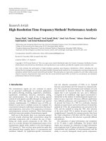
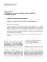
Figure 1: (a) The X-ray C-arm system in a clinical intervention. (b) The degrees of rotational freedom of the C-arm geometry. (c) A 3D data
set, acquired using the X-ray C-arm system.
We applied the presented approach to visualize intraop-
eratively acquired 3D data sets on a Philips 42

lenticular
screen, which was mounted in the operation room (OR).
The orientation of the 3D data set followed in realtime the
orientation of an X-ray C-arm system; see Figure 1. This
approach aids in reducing the X-ray radiation, since the
physician can choose the optimal orientation to acquire X-
ray images without actually radiating. Further, it improves
the interpretation of the live projective 2D X-ray image,

which is presented on a separate display, since the 3D data set
on the stereoscopic screen (which is in the same orientation)
gives a proper depth impression through the stereovision of
the lenticular screen. In this application, interactivity is very
important, and the refresh rate has to be sufficient to provide
a realtime impression. After all, when the refresh rate is too
low, the interaction with the human operator can lead to
oscillating manipulation. Further, the fact that the clinician
is not limited to single sweet spot makes these displays
particularly suitable for this environment, since the clinical
intervention demands that the operator can be positioned
freely in the range close to the patient.
2. State of the Art
In 1838, Sir Charles Wheatstone developed a device, called
the stereoscope, which allowed the left and the right eyes
to be presented with a different image (illustration or
photograph), in order to create an impression of depth.
Matusik and Pfister [2] presented a comprehensive overview
of the various systems for stereoscopic visualizations that
have been developed over the time. The development of auto
stereoscopic display devices, presenting stereoscopic images
without the use of glasses, goggles, or other viewing aids, has
seen an increasing interest since the 1990s [3–5].
The advancement of large high resolution LCD grids,
with sufficient brightness and contrast, has brought high-
quality multiview autostereoscopic lenticular displays within
reach [6]. A number of publications have investigated the
image quality aspects of autostereoscopic displays. Seunti
¨
ens

et al. [7] have discussed the perception quality of lenticular
displays as a function of white noise. Konrad and Agniel
[8] describe the Fourier domain properties of the lenticular
display, and they propose a pre-filtered sample approach. The
effect of light that ought to be contributed to one particular
view leaking into other views, which is called crosstalk, has
been quantitatively investigated by Brasspenning et al. [9]
and Boev et al. [10].
The range of viewing positions, allowing the perception
of a stereoscopic image, is mainly determined by the number
of views, offered by the display. Further, a higher resolution
per view leads to less artifacts and improves the image
quality. The required resolution of the LCD pixel grid can be
established as the number of views times the resolution per
view. Clearly, fulfilling both requirements demands very high
resolution LCD pixel grids, which means that an enormous
amount of pixel data has to be rendered and transferred to
the display.
Several publications describe how the GPU can be
employed to extract the data stream for the lenticular display
from a 3D scene in an effective manner. Kooima et al. [11]
present a two-pass GPU-based algorithm for two-view head-
tracked parallax barrier display. First the views for the left
and the right eyes are rendered, and in the subsequent pass
they are interweaved. Domonkos et al. [12]describeatwo-
pass approach, dedicated for isosurface rendering. In the first
pass they perform the geometry calculations on the pixel-
shader for every individual pixel, and in the second pass the
shading is performed. H
¨

ubner and Pajarola [13]describea
GPU-based single-pass multiview volume rendering, varying
the direction of the casted rays depending on their location
on the lenticular screen.
The previous GPU-based approaches were dedicated
render methods, working on the native resolution of the
lenticular LCD grid. We present an approach that decouples
the render resolution from the native LCD grid resolution,
allowing lower resolutions, when higher frame rates are
demanded.
3. The Multiview Lenticular Display
Multiview autostereoscopic displays can be regarded as
three-dimensional light field displays [14, 15](orfour-
dimensional, when also considering time). The dimensions
EURASIP Journal on Advances in Signal Processing 3
1
2
3
4
5
6
7
(a)
View: −1
0
1
(b)
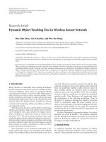
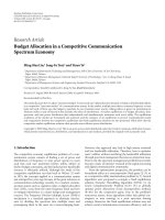
Figure 2: (a) The spatial multiplexing of the different views. (b)
The light of the subpixels is directed into different directions by the
lens [9].

−2
−3
−4
0
−1
−2
2
1
0
4
3
2
−3
−4
4
−1
−2
−3
1
0
−1
3
2
1
−4
4
3
−2
−3
−4

0
−1
−2
2
1
0
4
3
2
−3
−4
4
−1
−2
−3
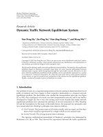
Figure 3: The cylindrical lenses depict every subpixel in a different
view. The numbers in the subpixels indicate in which view they are
visible.
are described by the parameters (x, y, φ), whereby x and y
indicate a position on the screen and φ indicates the angle in
the horizontal plane in which the light is emitted. The light
is further characterized by its intensity and its color.
The multiview lenticular display device consists of a
sheet of cylindrical lenses (lenticulars) placed on top of an
LCD in such a way that the LCD image plane is located
at the focal plane of the lenses [16]. The effect of this
arrangement is that LCD pixels located at different positions
underneath the lenticulars fill the lenses when viewed from
different directions; see Figure 2. Provided that these pixels
are loaded with suitable stereo information, a 3D stereo effect

is obtained, in which the left and right eyes see different,
but matching information. The screen we used offered nine
distinct angular views, but our method is applicable to any
number of views.
The fact that the different LCD pixels are assigned to
different views (spatial multiplex) leads to a lower resolution
per view than the resolution of the LCD grid [17]. In order
to distribute this reduction of resolution over the horizontal
and vertical axes, the lenticular cylindrical lenses are not
placed vertically and parallel to the LCD column, but slanted
at a small angle [1]. The resulting assignment of a set of LCD
pixels, which is specified by the manufacturer, is illustrated
in Figure 3. Note that the red, green, and blue color channels
of a single pixel are depicted in different views.
Projection matrix
view 1
Projection matrix
view 2
.
.
.
Projection matrix
view n
Volume rendering
Volume rendering
.
.
.
Volume rendering
Compositing Display

Figure 4: The process of rendering for the lenticular display.
Optionally, the rendering of the n individual views can be done in
parallel.
d
f
Screen
Figure 5: The frustums resulting from three different view points.
4. The Different Angular Views
We propose a two-pass algorithm: first the individual views
from the different foci positions are separately rendered to an
orthogonal grid. In the second pass, the final output signal
has to be resampled from the views to a nonorthogonal
grid in the compositing phase (see Figure 4). The processing
power of the GPU is harvested for both passes. In order to
maintain an acceptable frame rate, the resolution of the views
can be changed dynamically.
The frustums that result from the different focal spots
are illustrated in Figure 5. The viewing directions of the
frustums are not parallel to the normal of the screen, except
for the centered one. Therefore the corresponding frustums
are asymmetric [18]. A world coordinate (x, y, z) that is
perspectively projected, using such an asymmetric frustum,
leads to the following view port coordinate v(x, y):
v(x, y)
=

(x −n·d)·f
f −z
+ n
·d,

y
·f
f −z

,(1)
whereby f denotes the focal distance, n the view number,
and d the distance between the view cameras. All parameters
should be expressed in the same metric (e.g., millimeters),
and the origin is placed in the center of the view port.
Figures 5 and 6 illustrate the process of rendering the
scene from focal spot positions with an offset to the center of
the screen. After the projection matrix has been established,
using (1), the scene has to be rendered for that particular
view. All views are stored in a single texture, which we
call texture1. In OpenGL, the views can be placed next to
4 EURASIP Journal on Advances in Signal Processing
(a) (b)
Figure 6:Thesamescenerenderedfromthemostleftandmost
right view points.
each other in horizontal direction, using the glViewport
command. The location of a pixel in view n in texture1 can
be found as follows:

t
=

1
2
+
n


N
+
2p
x
−1
2

N
, p
y

,(2)
whereby

t denotes the normalized texture coordinate,

p the
normalized pixel coordinate within the view, and

N the total
number of views. The view index n is here assumed to be in
the range [
−(

N −1)/2, (

N −1)/2], as is used in, for example,
Figure 3.
5. Direct Volume Rendering

For each view the volumetric data set has to be rendered,
using the appropriate frustum perspective projection. In
order to use the GPU for volume rendering, the voxel data set
has to be loaded in the texture memory of the graphics card.
To obtain textures which are better suited for the memory
architecture of the graphics hardware and to be able to deal
with data set sizes exceeding the available texture memory,
the data set is divided into the so-called bricks.
The actual direct volume rendering process consists of
evaluating the volume rendering equation for rays which are
casted through the pixels of display; see Figure 7.Thevolume
rendering equation can be approximated by the following
summation:
i
=
M

m=0

α
m
c
m
·
m

m

=0


1 −α
m



,(3)
whereby i denotes the resulting color of a ray, α
m
the opacity
at a given sample m,andc
m
the color at the respective sample.
Since medical data sets typically only consist of scalar values,
a transfer function has to be defined, mapping the scalar
values to color and opacity values.
ThissummationcanbebrokendowninM iterations
over the so-called over operator [19], whereby the rays are
traversed in a back-to-front order:
C
m+1
= α
m
·c
m
+

1 −α
m

·C

m
. (4)
Here C
m
denotes the intermediate value for a ray. For (4),
standard alpha blending, offered by DirectX or OpenGL, can
Focal
spot
Display
Sample
Te x t u r e d
slice
Ray
(a)
(b) (c)
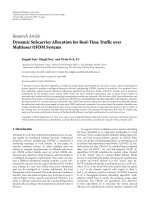
Figure 7: (a) Volume rendering involves the evaluation of the
volume render equation along the rays, passing through the pixels of
the display. The usage of textured slices means that the rays are not
evaluated sequentially. Rather for a single slice the contribution of
the sample points to all rays is processed. (b) A volume rendered
data set, with large intervals between the textured slices. (c) The
same volume rendered data set, with a small distance between the
textured slices.
be used. In order to execute (4), a set of textured slices,
containing the volumetric medical data, are blended into
each other [20]. To map the slices properly on the display
area, the projection matrix is set to match the perspective
defined by the focal spot and the display area; see (1). The
modelview matrix is a rigid transformation matrix, and
determines the position, orientation, and scale of the volume

in the 3D space. The slices are then processed in a back-to-
front order, whereby the intermediate results C
m
are written
in the frame buffer.
Our GPU-based direct volume rendering implementa-
tion is capable of rendering highlights, diffuse, and ambient
lighting, which enhances the depth impression. Further it can
handle any perspective projection matrix.
The rendered views are stored locally on the graphics
card. They are put horizontally next to each other, in a single
wide rectangular texture map; see Section 4. The fact that
the entire scene has to be drawn multiple times is partially
compensated by the fact that the individual views have a
lower resolution than the output window.
6. Resolution Considerations
The maximum information density that can be conveyed
by the lenticular display per view is determined by the way
the pixels of the LCD grid are refracted by the lenticular
lenses. In modern lenticular displays, the lens array is slanted
under a slight angle, which affects the distribution of the
set of pixels that are diverted to a particular viewing angle.
EURASIP Journal on Advances in Signal Processing 5
In Figure 9(a), it is shown how the green subpixels, visible
from the middle viewing position (view 0), are distributed
over the LCD grid. Though the allocation of the subpixels
over the grid is regular, it is not orthogonal. The sampling
theory of multidimensional signals, described by Dubois
[21], can be used to examine the frequency range that can
be transmitted by a certain nonorthogonal grid. Especially

the maximum view port size that does not lead to aliasing
is of interest. When the resolution of the view port is too
high, the compositing undersamples the view, and aliasing
occurs. Though such views can be low-pass filtered to prevent
aliasing, it is preferable to render them immediately at the
optimal resolution, in order to keep the load on the scarce
processing resources as low as possible.
The set of subpixels that are refracted to the same angular
view can be considered to form a lattice. Let the vectors
{

v
1
,

v
2
, ,

v
N
} form a basis, not necessarily orthogonal, of
R
N
. Then lattice Λ ⊂ R
N
is defined as a set of discrete
points in
R
N

, formed by all linear combinations of vectors

v
1
,

v
2
, ,

v
N
with integer coefficients.
In order to perform a Fourier transform of a signal,
sampled on a lattice, the reciprocal lattice is required. The
reciprocal lattice Λ
∗
of lattice Λ is defined as the set of vectors

y, such that

y
·

x is an integer for all

x
∈ Λ.LetV be the
matrix, whose columns are the representation of the basis
vectors


v
1
,

v
2
, ,

v
N
in the standard orthonormal basis for
R
N
. Then matrix W, containing the basis vectors of the
reciprocal lattice Λ
∗
, is determined by W
T
V = I,withI
being the N
·N identity matrix.
The Vorono i cell of a lattice is defined as the set of all
points in
R
N
closer to origin

0 than to any other lattice point;
see Figure 8. The basis V for a given lattice is not unique (i.e.,

alatticeΛ can be described by several different basis matrices
V). However, any basis for a certain lattice Λ delivers the
same unique Voronoi cell.
Let the Fourier transform of a continuous multidimen-
sional signal u
c
(

x)with

x ∈ R
N
be defined as
U
c


f

=

R
N
u
c


x

e

−j2π

f ·

x
d

x,

f ∈ R
N
. (5)
The Fourier transformation of signal u
c
sampled on lattice Λ
is periodical, with lattice Λ
∗
as periodicity [21]:
U


f

=
1


det V





r
∈Λ
∗
U
c


f +

r

. (6)
Consequently, if a signal that is not bandwidth limited within
the Voronoi cell of lattice Λ
∗
is sampled on lattice Λ,spectral
overlap (i.e., aliasing) occurs.
The sampling that occurs in the compositing phase can
be examined, considering only one monochromatic primary
color (red, green, or blue), or can be evaluated for all
colors together; see Figure 9. The basis matrices V of the
sample lattice can be established by taking two vectors
(nonlinearly dependent) between adjacent lattice points. The
LCD pixel distance is used as a metric, which means that two
neighboring subpixels (e.g., red and green) have a distance
of 1/3 pixel. For example, for the color-independent lattice
Figure 8: A lattice (black dots) and corresponding Voronoi cells
(red). The green vectors compose a possible basis V for this lattice.

The Voronoi cell of a given lattice point is the set of points in
R
N
that are closer to this particular lattice point than to any other lattice
point.
(Figure 9(b)), we take the vectors

v
1
= (5/3, −1)
T
and

v
2
=
(4/3, 1)
T
. This delivers the following basis matrices V and
their reciprocals W
T
:
V
mono
=

3 −1
0
−3


, V
color
=
⎛
⎝
5
3
4
3
−11
⎞
⎠
,
W
mono
=
1
9

30
−1 −3

, W
color
=
1
9

33
−45


.
(7)
The individual views are rendered on an orthogonal grid,
and the Voronoi cell of an orthogonal lattice is a simple
rectangle. The maximum resolution that can be visualized on
the lenticular screen can be examined by fitting this Nyquist
frequency rectangle range of the orthogonal grid on the
Voronoi cell of the reciprocal lattice of the lenticular sample
grid.
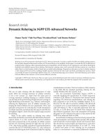
A logical choice for the resolution of the individual views,
for a lenticular screen with 9 views, seems to be 1/3 of the
LCD pixel grid resolution in both directions. After all, this
represents the same amount of information: 9 views with
each 1/3
·1/3· the amount of pixels of the LCD grid. We
call this the 1/3 orthogonal grid. The Nyquist frequency
rectangle of this resolution has been depicted on top of the
Voronoi cell of the reciprocal lattice of the lenticular sample
grid in Figure 9. Looking at a single primary color channel
(in Figure 9(a) the green subpixels are used, but the lattice
is the same for red and blue), it can be noted that the
rectangle is not completely encapsulated within the Voronoi
cell. This means that for monochromatic red, green, and blue
images there is a slight undersampling in certain directions,
and aliasing might occur in the higher frequencies. If the
lenticular lattice for a single view is considered, regardless of
the colors of the subpixels, then the rectangle is completely
contained within the Voronoi cell; see Figures 9(b) and
9(d). This implies that for gray colored images there is no

aliasing when only the intensities are considered, but there
might be some aliasing between the colors. In practise, this
behavior resembles color dithering for real-world images.
6 EURASIP Journal on Advances in Signal Processing
−2
−3
−4
4
0
−1
−2
−3
2
1
0
−1
4
3
2
1
−3
−4
4
3
−1
−2
−3
−4
1
0

−1
−2
3
2
1
0
−4
4
3
2
−2
−3
−4
4
0
−1
−2
−3
2
1
0
−1
4
3
2
1
−3
−4
4
3

−1
−2
−3
−4
(a)
−2
−3
−4
4
0
−1
−2
−3
2
1
0
−1
4
3
2
1
−3
−4
4
3
−1
−2
−3
−4
1

0
−1
−2
3
2
1
0
−4
4
3
2
−2
−3
−4
4
0
−1
−2
−3
2
1
0
−1
4
3
2
1
−3
−4
4

3
−1
−2
−3
−4
(b)
(c) (d)
Figure 9: (a) The LCD pixel grid and the view that is associated with each subpixel. The green subpixels that are diverted to view 0 are circled.
(b) All subpixels that are diverted to view 0 are circled, independent from their color. (c) The reciprocal lattice of the green subpixels for
view 0. The Voronoi cell of the reciprocal lattice is indicated in pink. In blue, the Nyquist frequency of the 1/3 orthogonal grid is indicated.
Since the Voronoi cell does not cover the complete Nyquist frequency range, slight aliasing in the higher frequencies might occur. (d) The
reciprocal lattice of the subpixel configuration of view 0, ignoring their color. Since the Nyquist frequency range (blue) is contained within
the Voronoi cell (pink), there is no aliasing in the intensity image.
High frequent primary-colored structures (such as thin lines)
may suffer from slight visible aliasing artifacts, though.
7. Dynamic Resolution
As long as there are sufficient processing resources available,
the resolution of the angular views is set to the 1/3 orthogonal
grid. This resolution provides a good tradeoff between
maximum detail and minimum aliasing, as described above.
When the frame rate falls below a predefined threshold,
the resolution of the individual views can be lowered; see
Figure 10.
For the sake of simplicity, we use the same resolution for
all views that contribute to a particular frame, but there is
no technical reason imposing this. The resolution of a view
can simply be changed by setting the view port to the desired
size. The size of the offscreen buffer containing texture1 is not
changed; it is always kept at the maximum size needed.
Of course, lowering the view resolution does not guaran-

tee that the desired minimum frame rate is achieved. This
is mostly determined by the major bottlenecks in the 3D
scene [20]. In cases where the major bottleneck is determined
by the fragment throughput, the frame rate scales very well
with the view port size, and may increase significantly. When,
for example, the vertex throughput is the most important
bottleneck, the frame rate is largely independent of the view
port size.
Lower-resolution views correspond to smaller Nyquist
rectangles in the frequency domain. For lower resolutions,
the rectangle typically fits in the Voronoi cell of Figure 9(c),
which implies that the view is oversampled by the com-
positing process. This corresponds to low-pass filtering the
view at maximum resolution, which means that reducing
dynamically the view resolution does not lead to aliasing
artifacts, but merely to loss of detail. These details can be
regained when the scene content is more static, and there is
sufficient time to render the scene at high resolution.
To composite the final image, which will be displayed on
the lenticular screen, the red, green, and blue components
of each pixel have to be sampled from a different view (see
Figure 3). The view number stays fixed all the time for each
subpixel. Therefore, this information is precalculated once,
and then put in a static texture map, called texture0.
In the compositing phase, all the pixels in the output
image are parsed by a GPU program. For each normalized
pixel coordinate

p in the output image, texture0 will deliver
EURASIP Journal on Advances in Signal Processing 7

(a) (b)
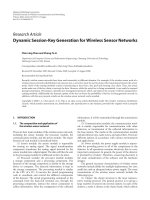
Figure 10: (a) The lenticular screen has been photographed to show how a view is being displayed, rendered at the 1/3 orthogonal grid
resolution. (b) The same view, but sampled at 0.375 the resolution of the view in (a). Though the downsampling is visible, the effect is less
strong than might be expected. This can be contributed to the fact that the displaying process possesses a low-pass filter character, due to
effects like crosstalk.
(a) (b)
Figure 11: (a) The raw output signal that is sent to the lenticular display. Please note that the Moir
´
e-like structures are not artifacts, but can
be contributed to the interweaved subpixels, belonging to different views. (b) A zoomed fragment of the left image.
the view numbers n that have to be sampled for the
red, green, and blue components. The respective views are
then sampled in texture1 according to (2), using bilinear
interpolation, delivering the appropriate pixel value; see
Figure 11.
8. Results and Conclusions
Figure 12 shows the adaptive adjustment of the view resolu-
tion. The minimum desired frame rate was set to 7 frames
per second in this case, which corresponds to rendering
63 views per second, since the lenticular display requires
nine views to compose one frame. The measurements were
performed using volume rendering of the data set depicted
in Figure 10, and involved advanced lighting. It consisted of
256
2
·200 voxels (25 MB), while the output signal comprised
1600
·1200 pixels. The resolution of the views was the
resolution of the 1/3 orthogonal grid, multiplied by the
scaling factor (right vertical axis) in both the x-andy-

directions.
In order to characterize the performance of the GPU-
accelerated volume rendering and compositing, several data
sets were rendered at the 1/3 orthogonal grid resolution to
an output window of 800
2
pixels. Nine views were rendered
per frame, and the view size was 264
2
pixels. Using a scan of
a foot, consisting of 256
2
·200 voxels (25 MB), we achieved
a frame rate of 52.4 frames per second, which corresponds
to rendering 471 views per second. A CT scan of a head of
512
2
·256 voxels (128 MB) could be rendered at 19.2 frames
per second (173 views per second), and a 3DRA data set of
8 EURASIP Journal on Advances in Signal Processing
0
1
2
3
4
5
6
7
8
9

10
(fps)
0
0.1
0.2
0.3
0.4
0.5
0.6
0.7
0.8
0.9
1
Scaling
Figure 12: Pink line: frame rate in frames per second (fps). Blue
line: view resolution scaling. The horizontal axis represents the
time.
512
3
voxels (256 MB), showing the vasculature in the brain,
could be visualized at 21.3 frames per second (192 views per
second).
All measurements were obtained, using a 2.33 GHz
Pentium 4 system, with 2GB RAM memory, and an nVidia
QuadroFX 3500 with 256 MB on board memory as graphics
card.
In this article, a method for accelerated direct volume
rendering to multiview lenticular displays has been pre-
sented. Due to the GPU-acceleration, together with the
adaptive adjustment of the intermediate view resolution,

interactive frame rates can be reached, which allows intuitive
manipulation of the rendered scene. Since both the volume
rendering and the compositing take place on the graphics
hardware, the requirements for the other components of the
PC system are rather modest. Thus the realization of the
proposed high-performance system can be very cost effective.
The fact that viewers do not need to wear any additional
glasses, and are not limited to a sweet spot, as well as the
fact that large data sets can be manipulated interactively,
make this method very suitable for a clinical interventional
environment.
References
[1]C.vanBerkel,D.W.Parker,andA.R.Franklin,“Multiview
3D LCD,” in Stereoscopic Displays and Virtual Reality Systems
III, vol. 2653 of Proceedings of SPIE, pp. 32–39, San Jose, Calif,
USA, January-February 1996.
[2] W. Matusik and H. Pfister, “3D TV: a scalable system for real-
time acquisition, transmission, and autostereoscopic display
of dynamic scenes,” ACM Transactions on Graphics, vol. 23, no.
3, pp. 814–824, 2004.
[3] M. Halle, “Autostereoscopic displays and computer graphics,”
ACM Computer Graphics, vol. 31, no. 2, pp. 58–62, 1997.
[4] N. A. Dodgson, “Autostereoscopic 3D displays,” Computer, vol.
38, no. 8, pp. 31–36, 2005.
[5] L. Onural, T. Sikora, J. Ostermann, A. Smolic, M. R. Civanlar,
and J. Watson, “An assessment of 3DTV technologies,” in
Proceedings of the 60th Annual NAB Broadcast Enginee ring
Conference, pp. 456–467, Las Vegas, Nev, USA, April 2006.
[6] A. Vetro, W. Matusik, H. Pfister, and J. Xin, “Coding
approaches for end-to-end 3D TV systems,” in Proceedings of

the 24th Picture Coding Symposium (PCS ’04), pp. 319–324,
San Francisco, Calif, USA, December 2004.
[7]P.J.H.Seunti
¨
ens, I. E. J. Heynderickx, W. A. IJsselsteijn, et
al., “Viewing experience and naturalness of 3D images,” in
Three-Dimensional TV, Video, and Display IV, vol. 6016 of
Proceedings of SPIE, pp. 43–49, Boston, Mass, USA, October
2005.
[8] J. Konrad and P. Agniel, “Subsampling models and anti-alias
filters for 3-D automultiscopic displays,” IEEE Transactions on
Image Processing, vol. 15, no. 1, pp. 128–140, 2006.
[9] R. Braspenning, E. Brouwer, and G. de Haan, “Visual quality
assessment of lenticular based 3D displays,” in Proceedings of
the 13th European Signal Processing Conference (EUSIPCO ’05),
Antalya, Turkey, September 2005.
[10] A. Boev, A. Gotchev, and K. Egiazarian, “Crosstalk measure-
ment methodology for autostereoscopic screens,” in Proceed-
ingsofthe3DTVConference, pp. 1–4, Kos Island, Greece, May
2007.
[11] R. L. Kooima, T. Peterka, J. I. Girado, J. Ge, D. J. Sandin, and T.
A. Defanti, “A GPU sub-pixel algorithm for autostereoscopic
virtual reality,” in Proceedings of the IEEE Virtual Reality (VR
’07), pp. 131–137, Charlotte, NC, USA, March 2007.
[12] B. Domonkos, A. Egri, T. F
´
oris,T.Juh
´
asz, and L. Szirmay-
Kalos, “Isosurface ray-casting for autostereoscopic displays,”

in Proceedings WSCG, pp. 31–38, Plzen, Czech Republic,
January-February 2007.
[13] T. H
¨
ubner and R. Pajarola, “Single-pass multiview volume
rendering,” in Proceedings of the IADIS International Con-
ference on Computer Graphics and Visualization (CGV ’07),
Lisbon, Portugal, July 2007.
[14] M. Levoy and P. Hanrahan, “Light field rendering,” in Pro-
ceedings of the 23rd Annual Conference on Computer Graphics
and Interactive Techniques (SIGGRAPH ’96), pp. 31–42, New
Orleans, La, USA, August 1996.
[15] A. Isaksen, L. McMillan, and S. J. Gortler, “Dynamically
reparameterized light fields,” in Proceedings of the 27th Annual
Conference on Computer Graphics and Interactive Techniques
(SIGGRAPH ’00), pp. 297–306, New Orleans, La, USA, July
2000.
[16] C. van Berkel, “Image preparation for 3D LCD,” in Stereoscopic
Displays and Virtual Reality Systems VI, vol. 3639 of Proceed-
ings of SPIE, pp. 84–91, San Jose, Calif, USA, January 1999.
[17] N. A. Dodgson, “Autostereo displays: 3D without glasses,” in
Proceedings of the Electronic Information Displays (EID ’97)
,
Surrey, UK, November 1997.
[18] D. Maupu, M. H. Van Horn, S. Weeks, and E. Bullitt,
“3D stereo interactive medical visualization,” IEEE Computer
Graphics and Applications, vol. 25, no. 5, pp. 67–71, 2005.
[19] T. Porter and T. Duff, “Compositing digital images,” ACM
Computer Graphics, vol. 18, no. 3, pp. 253–259, 1984.
[20] D. Ruijters and A. Vilanova, “Optimizing GPU volume

rendering,” Journal of WSCG, vol. 14, no. 1–3, pp. 9–16, 2006.
[21] E. Dubois, “The sampling and reconstruction of time-varying
imagery with application in video systems,” Proceedings of the
IEEE, vol. 73, no. 4, pp. 502–522, 1985.