Báo cáo hóa học: " Research Article Distributed Iterative Multiuser Detection through Base Station Cooperation" pot

Hindawi Publishing Corporation
EURASIP Journal on Wireless Communications and Networking
Volume 2008, Article ID 390489, 15 pages
doi:10.1155/2008/390489
Research Article
Distributed Iterative Multiuser Detec tion through
Base Station Cooperation
Shahid Khattak, Wolfgang Rave, and Gerhard Fettweis
Vodafone Chair Mobile Communications Systems, Technische Universit
¨
at Dresden, 01062 Dresden, Germany
Correspondence should be addressed to Shahid Khattak,
Received 1 August 2007; Revised 18 December 2007; Accepted 13 February 2008
Recommended by Huaiyu Dai
This paper deals with multiuser detection through base station cooperation in an uplink, interference-limited, high frequency
reuse scenario. Distributed iterative detection (DID) is an interference mitigation technique in which the base stations at different
geographical locations exchange detected data iteratively while performing separate detection and decoding of their received data
streams. This paper explores possible DID receive strategies and proposes to exchange between base stations only the processed
information for their associated mobile terminals. The resulting backhaul traffic is considerably lower than that of existing
cooperative multiuser detection strategies. Single-antenna interference cancellation techniques are employed to generate local
estimates of the dominant interferers at each base station, which are then combined with their independent received copies from
other base stations, resulting in more effective interference suppression. Since hard information bits or quantized log-likelihood
ratios(LLRs)aretransferred,weinvestigatetheeffect of quantization of the LLR values with the objective of further reducing
the backhaul traffic. Our findings show that schemes based on nonuniform quantization of the “soft bits” allow for reducing the
backhaul to 1–2 exchanged bits/coded bit.
Copyright © 2008 Shahid Khattak et al. This is an open access article distributed under the Creative Commons Attribution
License, which permits unrestricted use, distribution, and reproduction in any medium, provided the original work is properly
cited.
1. INTRODUCTION
An ever growing demand for new broadband multimedia
services emphasizes the need for higher spectral efficiency in

future wireless systems. A higher-frequency reuse is therefore
proposed, resulting in the interference from cochannel users
outside the cells to dominate, thereby forming a single
most important factor limiting the system performance.
This interference coming from outside the cell boundaries
is commonly referred to as other cell inter ference (OCI). OCI
has been treated in [1], where it was suggested that advanced
receiver and transmitter techniques can be employed in the
uplink and downlink of a cellular system, respectively. Given
that the mobile terminals (MTs) are low-cost, low-power
independent entities, and are not expected to cooperate to
perform transmit or receive beamforming, they are assumed
to be as simple as possible with most of the complex
processing of a cellular system moved to the base stations
(BSs).
In this paper, we restrict ourselves to advanced receiver
techniques for uplink communication. Different advanced
receiver techniques, suggested in the literature for the
uplink, give tradeoffs between complexity and performance.
Optimum maximum likelihood detection (MLD) [2, 3]is
prohibitively complex for multiple-input multiple-output
(MIMO) scenarios employing higher-order modulation.
Linear receivers [4–7] are simpler, but less effective in
decoupling the incoming multiplexed data streams, and offer
low spatial diversity for full-rank systems. Iterative receivers
[8–10] with soft decision feedback offer the best compromise
between complexity and performance, and they have been
universally adopted as a strategy of choice.
One principal line of thought to address the OCI
problem was initiated by Wyner ’s treatment of base station

cooperation in a simple and analytically tractable model of
cellular systems [11]. In this model, cells are arranged in
either an infinite linear array or in some two-dimensional
pattern, with interference originating only from the imme-
diate neighboring cells (having a common edge). All the
processing is performed at a single central point. Subsequent
work on the information theoretic capacity of the centralized
processing systems concluded that the achievable rate per
2 EURASIP Journal on Wireless Communications and Networking
user significantly exceeds that of a conventional cellular
system [12, 13].
Recently, decentralized detection using the belief propa-
gation algorithm for a simple one-dimensional Wyner model
was proposed in [14]. The belief propagation algorithm
effectively exchanges the estimates for all signals received
at each BS, by alternately exchanging likelihood values
and extrinsic information. This idea was extended to 2D
cellular systems in [15–17], where the limits compared to
MAP decoding were studied, showing the great potential
of BS cooperation with decentralized processing (at least
for regular situations). Unfortunately, for a star network
(commonly used today) interconnecting the BSs, this results
in a huge backhaul traffic.
Another approach to convert situations where cochannel
users interfere each other with comparably strong signals
into an advantage for a high-frequency reuse cellular system
was proposed in [18]: different BSs cooperate by sending
quantized baseband signals to a single central point for joint
detection and decoding. Such a distributed antenna system
(DAS) not only reduces the aggregate transmitted power, but

also results in much improved received SINR [19]. Using
appropriate receive strategies, both array and diversity gains
are obtained, resulting in a substantial increase in system
capacity [20, 21]. The DAS scheme, however, is less attractive
for network operators due to the large amount of backhaul
it requires and the cooperative scheduling necessary between
the adjacent DAS units in order to avoid interference. Here,
backhaul is defined as the additional communication link
between different cooperating entities. Although the band-
width of wired links used for backhaul can be very high, they
are usually owned by a third party, making it attractive for the
cellular system operators to reduce the backhaul in order to
minimize operating costs. The influence of limited backhaul
on capacity in DAS has been investigated in [22, 23].
Similarly as in the mentioned works, we are interested
in asymmetric multiuser detection scenarios. We assume
that the resource management of the cellular network can
detect (e.g., via signal strength indicators) groups of MTs
that are strongly received at several base stations. However,
in contrast to [15, 17] and related work, our main interest
is not the network wide optimum information exchange,
but rather its decentralized implementation. To this end,
the concept of distributed iterative detection (DID) was
introduced in [24, 25]: each base station initially performs
single-user detection for the strongest MT, treating the
signals received from all other mobile terminals as noise. The
information that becomes available at the decoder output
is then sent to neighboring BS while mutually receiving
data from its own neighbors in order to reconstruct and
cancel the interference of its own received signal. Single-user

detection is then applied to this interference-reduced signal
by applying parallel interference cancellation [26]. Further
improvements can be achieved by repeated application of
this procedure. The questions we try to answer here are as
follows.
(i) How much improvement can we get with respect
to conventional single-user detection in different scenarios
(varying strength of the user coupling through the channel)?
(ii) Which additional gain is possible if we replace the
single-user detection step in the 0th iteration with
single-antenna interf erence cancellation (SAIC) which is
implemented as j oint maximum likelihood detection (JMLD)
in the symbol detector acting as the receiver frontend?
(iii) What is a reasonable trade off between the amount
of information exchange and improvement beyond single-
user detection? Or, stated otherwise, what happens under
constraints for the maximum available data rate over the
backhaul links between base stations and associated finite
precision effects due to quantization?
The organization of the remainder of this paper is as
follows. Section 2 presents the system model, where the
coupling among users/cells and the channel model are
described. Section 3 discusses in detail various components
of distributed iterative receivers. In Section 4 different decen-
tralized detection strategies are compared. In Section 5 we
examine the effect of quantization of reliability information.
We compare various quantization strategies in terms of
information loss and necessary backhaul traffic. Numerical
results are presented in Section 6 before conclusions are
drawn.

Notation
Throughout the paper, complex baseband notation is used.
Vectors are written in boldface. A set is written in double
stroke font such as
I and its cardinality is denoted by |I|.
The expected value and the estimates of a quantity such as s
are denoted as E
{s} and s,respectively.Randomvariablesare
written as uppercase letters and their realization with lower-
case letters. A posteriori probabilities (APPs) will be expressed
as log-likelihood ratios (L-values). A superscript denotes
the origin (or receiver module), where it is generated. We
distinguish L
d1
, L
d2
,andL
ext
which are APPs generated at the
detector and the decoder of a given BS or externally to it.
2. TRANSMISSION MODEL
We consider an idealized synchronous single-carrier (narrow
band) cellular network in the uplink direction. N is the
number of receive antennas and M is the number of transmit
antennas corresponding to the number of BSs and cochannel
MTs, respectively.
A block of information bits u
m
from user antenna m is
encoded and bit-interleaved leading to the sequence x

m
of
length K,wherem
= 1···M. This sequence is divided into
groups of q bits each, which are then mapped to a vector of
output symbols for user m of size K
s
= K/q according to s
m
=
[s
m,1
, , s
m,K
s
] = map(x
m
). Each symbol is randomly drawn
from a complex alphabet
A of size Q= 2
q
with E{s
m,k
}=0
and E
{|s
m,k
|
2
}=σ

2
s
for m = 1 ···M.
AblockofK
s
symbol vectors s[k] = [s
1,k
, s
2,k
, , s
M,k
]
T
(corresponding to one respective codeword) is transmitted
synchronously by all M users. At any BS l, a corresponding
block of symbols r
l
[k] is received, where the index k is related
to time or subcarrier indices (1
≤ k ≤ K
s
):
r
l
[k] = g
l
[k]·s[k]+n[k], 1 ≤ k ≤ K
s
. (1)
Shahid Khattak et al. 3

With n we denote the additive zero mean complex Gaussian
noise with variance σ
2
n
= E{n
2
}. For ease of notation, we
omit the time index k in the following, because the detector
operates on each receive symbol r
l
separately.
The row vector g
l
is the elementwise product g
l,m
=
h
l,m
√
ρ
l,m
of weighted channel coefficients h
l,m
of M co-
channels seen at the lth BS. The channel coefficient vector
h
l
, obtained as the current realization of a channel model
(the channel is passive on the average, i.e., E
{|h

l,m
|
2
}=1),
is assumed to be known perfectly. The coupling coefficients
ρ
l,m
reflect different user positions (path losses) with respect
to base station l. These will be abstracted in the following by
two coupling coefficients ρ
i
and ρ
j
which characterize the BS
interaction with strong and weak interferers.
Equation (1) can therefore be written in terms of the
desired signal (denoted with the index d) and weak and
strong interferences:
r
l
= g
ld
s
d
+

i∈I
l
g
li

s
i
+

j∈I
l
g
lj
s
j
+ n
= h
ld
s
d
+

ρ
i

i∈I
l
h
li
s
i
  
strong interference
+


ρ
j

j∈I
l
h
lj
s
j
  
weak interference
+ n,
(2)
where ρ
ld
= 1. We note that this is of course a variant of
the two-dimensional Wyner model. With
I
l
we denote the
set of indices of all strongly received interferers at BS l with
cardinality
|I
l
|=m
l
−1, where m
l
is total number of strongly
received signals at BS l. Additionally,

I
l
is the complementary
set for all weakly received interferers:
|I
l
∪I
l
|=M − 1.
Note that the received signal-to-noise ratio (SNR) is
defined as the ratio of received signal power at the nearest
BS and the noise power. Specifically, the SNR at the lth BS
can be written as SNR
= E{h
ld
s
d

2
}/E{n
2
}=σ
2
s
/σ
2
n
.
The considered synchronous model is admittedly some-
what optimistic and was recently criticized due to the impos-

sibility to compensate different delays to different mobiles
(positions) simultaneously [27]. However, the reason to
ignore synchronization errors is twofold. First, it allows
to study the possible improvement through base station
cooperation without other disturbing effects to obtain
bounds (the degradation from nonideal synchronization
should thereafter be included as a second step). Second,
for OFDM transmission or frequency domain equalization
that we envisage in order to obtain parallel flat channels
enabling separate JMLD on each subcarrier, we argue that
it is possible to keep the interference due to timing and
frequency synchronization errors at acceptable levels.
Increased delay spreads of more distant MTs have to
be handled by an appropriately adjusted guard interval in
the cooperating region. Timing differences between mobiles
lead to phase shifts in the channel transfer function,
which are taken into account with the channel estimate.
Concerning frequency offsets due to variations among
oscillators and Doppler effects, one has to evaluate the
intercarrier interference induced by relative shifts of the
subcarrier spectra of different users. Roughly estimating
this with the sinc
2
( f/f
sub
) function of the power spectral
density for adjacent subcarriers, the SINRshould still be
Cell 1 Cell 2
Cell 4 Cell 3
d

44
d
14
d
33
d
13
d
11
d
12
d
22
BS
MT
ρ
11
=

d
11
d
11

γ
= 1  ρ
Th
ρ
12
=


d
22
d
22

γ
≈ 1  ρ
Th
⎫
⎪
⎪
⎪
⎬
⎪
⎪
⎪
⎭
Strong signals
ρ
13
=

d
33
d
13

γ
<ρ

Th
ρ
14
=

d
44
d
14

γ
<ρ
Th
⎫
⎪
⎪
⎪
⎬
⎪
⎪
⎪
⎭
Weak signals
γ: Path-loss exponent
d
lm
: Distance b/w BS l and MT m
Figure 1: An example setup showing a rectangular grid of 4 cells,
with power control assumed with respect to associated BS.
well above 20 dB, if the frequency offset can be kept at the

order of 1% and therefore become negligible with respect
to the interference to be cancelled on the same resource
(oscillator accuracies of 0.1 ppm considered, e.g., in the
LTE standardization translate to around 1% in terms of
the subcarrier spacing of 15 kHz). We, however, leave the
detailed study of asynchronous transmission for future work.
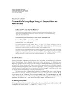
As an example for a cellular scenario that we intend to
capture with our model, a rectangular grid of 4 cells is shown
in Figure 1,whereρ
Th
is the path-loss threshold introduced
to distinguish between weak and strong interferers. It is
defined as the minimum path loss required for an interferer
to be detected separately during the BS processing. It depends
upon the constellation size and m
l
; for example, for 16-QAM
and m
l
= 2weuseρ
Th
=−12dB. Periodic or nonperiodic
boundary conditions are possible, allowing for representing
extended joint operation or isolated groups of cooperating
BSs.
3. DISTRIBUTED ITERATIVE RECEIVER
The setup for performing distributed detection with infor-
mation exchange between base stations is shown in Figure 2.
It comprises one input for the signal r
l

generated by the
mobile terminals and received at the base station antenna. In
addition, it contains a communication interface for exchang-
ing information with the neighboring base stations. This
information is either in the form of hard bits
u
l
or likelihood
ratios L
d2
l
of the locally detected signal and corresponding
quantities about the estimates of the interfering signals
delivered from other base stations. This communication
interface is capable of not only transmitting information
about the detected data stream to the other base stations, but
also receiving information from these base stations.
The receiver processing during initial processing involves
either SAIC/JMLD or conventional single-user detection
followed by decoding. In subsequent iterations, interfer-
ence subtraction is performed followed by conventional
single-user detection and decoding. Different components
of the distributed multiuser receiver are discussed in what
follows:
(i) interference cancellation,
(ii) demapping at the symbol detector,
4 EURASIP Journal on Wireless Communications and Networking
g
l
·s

i
Soft
modulator
s
i
μ
ext
i
/

L
ext
i
π
π
−1

L
tot
i
=

L
d2
i
+

L
ext
i

Extrinsic info. from
neighboring BS
+
+
−
Encoder
u
d
/L
d2
d
r
l
y
l
Detector Decoder
L
d2
d
L
a2
d
,
†
L
a2
i
L
d1
d

,
†
L
d1
i
†
L
d2
i
σ
2
eff
Figure 2: A DID receiver at the lth base station. The subscripts
d and i represent the desired data stream and the dominant
interferers. Variables designated by
† are evaluated only in the first
pass of the processing through the receiver. The superscripts 1 and
2 correspond to variables associated with detector and decoder,
respectively.
(iii) soft decoding,
(iv) (soft) interference reconstruction.
3.1. Interference canceller and effective
noise calculation
At the beginning of every iterative stage, interference of
neighboring mobile terminals is subtracted from the signal
received at each base station. If r
l
is the signal received at
the lth base station, the interference-reduced signal y
l

at the
output of the interference canceller is
y
l
= r
l
− g
l
·s
i
= r
l
−

i∈I
l
∪I
l
g
li
s
i
,(3)
where
s
i
∈ C
[1×n
T
]

is a vector of symbol estimates. If we
exchange only hard decisions about the information bits,
then no reliability information is conveyed. Under such
condition, additional noise due to the variance of the symbol
estimates is not available and the effective noise variance σ
2
eff
is underestimated and taken to be equal to that of receiver
input noise, that is, σ
2
eff
= σ
2
n
. On the other hand, if reliability
information for the received bits is available, a vector of
error variances e
2
i
for the estimated symbol streams can
be calculated. It is then added to the AWGN noise for the
subsequent calculations:
σ
2
eff
= σ
2
n
+


i∈I
l
∪I
l


g
li


2
E



s
i
− s
i


2

= σ
2
n
+

i∈I
l

∪I
l


g
li


2
e
2
i
  
residual-noise
.
(4)
The quantities e
2
i
and s
2
i
are both evaluated in the soft mod-
ulator (see Figure 1) and are discussed in detail in
Section 3.4.
Note that if the contributions of weak interferers
s
i
∈ I
l

in (4)and(5) are neglected, an error floor will occur in the
performance curves, especially at higher-order modulation.
Since both e
2
i
and s
2
i
are evaluated upon arrival of esti-
mates from the neighboring base stations, the interference
subtractor is not activated during the first pass and r
l
is fed
directly into the detector. The effective noise due to inherent
interference present in the signal during the first pass is
calculated based on the mean transmitted signal power and
the number m
d
of received signals that are to be jointly
detected. Therefore, for the first pass, the effective noise σ
2
eff
at the input of the detector of the lth BS, assuming m
d
= m
l
,
is given as
σ
2

eff
= σ
2
n
+ σ
2
s

i∈I
l


g
li


2
. (5)
3.2. Detection and demapper APP evaluation
The interference-reduced signal y
l
and its corresponding
noise value are sent to a demapper to compute the a
posteriori probability, usually expressed as an L-value [28]. If
m
d
data streams (each with q bits/sample) are to be detected,
the a posteriori probabilities L
d1
(x

k
|y
l
)ofthecodedbits
x
k
∈{±1} for k = 1 ···qm
d
, conditioned on the input
signal y
l
,aregivenas
L
d1

x
k
|y
l

=
ln
P

x
k
= +1|y
l

P


x
k
=−1|y
l

. (6)
For m
d
= 1 single-user detection is applied. When m
d
= m
l
,
(where m
l
is the number of strong signals at the BS l)JMLD-
based single-antenna interference cancellation is applied.
We make the standard assumption that the received bits
from any of the m
d
data streams in y
l
have been encoded
and scrambled through an interleaver placed between the
encoder and the modulator. Therefore, all bits within y
l
can be assumed to be statistically independent of each
other. Using Bayes’ theorem and exploiting the independence
of x

1
, x
2
, , x
qm
d
by splitting up joint probabilities into
products, we can write the APPs as
L
d1

x
k
|y
l

= ln
P

y
l
|x
k
= +1

P

x
k
= +1


P

y
l
|x
k
=−1

P

x
k
=−1

=
ln

x∈X
k,+1
p

y
l
|x


x
i
∈x

P

x
i


x∈X
k,−1
p

y
l
|x


x
i
∈x
P

x
i

.
(7)
X
k,+1
is the set of 2
qm
d

−1
bit vectors x having x
k
= +1, and
X
k,−1
is the complementary set of 2
qm
d
−1
bit vectors x having
x
k
=−1; that is,
X
k,+1
=

x|x
k
= +1

, X
k,−1
=

x|x
k
=−1


. (8)
The product terms in (7) are the a priori information about
the bits belonging to a certain symbol vector. Since we do not
make use of any a priori information in the demapper, these
termscancelout.TheL-values at the output of the demapper
can now be obtained by taking the natural logarithm of the
ratio of likelihood functions p(y
l
|x), that is,
L
d1

x
k
|y
l

= ln

x∈X
k,+1
p

y
l
|x


x∈X
k,−1

p

y
l
|x

. (9)
Shahid Khattak et al. 5
Calculating likelihood functions
The signal y
l
at the detector input contains not only m
d
signals that are to be detected at a BS, but also noise
and weak interference. For a typical urban environment
(assumed here), the number of cochannel interferers from
the surrounding cells can be quite large. We therefore make
the simplifying assumption that the distribution of the
effective noise due to the (M
− m
d
) interferers together
with the receiver noise is Gaussian. The likelihood function
p(y
l
|s
d
) can then be written as
p


y
l
|s
d

=
1
πσ
2
eff
exp

−
1
σ
2
eff

y
l
− h
ld
s
d
−

i∈I
l
g
li

s
i

2

,
(10)
where s
d
= map(x) is the vector of m
d
jointly detected
symbols. For single-user detection, s
d
= s
d
and the sum
term in the exponent of (10) disappears (the subscript “d”
in m
d
and s
d
denotes the detected streams). This should not
be confused with the desired user meant by the scalar s
d
.
To e v a l u a t e ( 10), the standard trick that we exploit in our
numerical simulation is the so-called “Jacobian logarithm”:
ln


e
x
1
+ e
x
2

= max

x
1
, x
2

+ln

1+e
−|x
1
−x
2
|

. (11)
The second term in (11) is a correction of the coarse
approximation with the max-operation and can be neglected
for most cases, leading to the max-log approximation. The
APP at the detector output at the lth BS as given in (9)can
then be simplified to
L

d1

x
k
|y
l

∼
=
max
x∈X
k,+1

−
1
σ
2
eff





y
l
− h
ld
s
d
−


i∈I
l
g
li
s
i





2

−
max
x∈X
k,−1

−
1
σ
2
eff





y

l
− h
ld
s
d
−

i∈I
l
g
li
s
i





2

.
(12)
Despite the max-log simplification, the complexity of calcu-
lating L
d1
(x
k
|y
n
) is still exponential in the number of the

detected bits in x. To find a maximizing hypothesis in (12)
for each x
k
, there are 2
qm
d
−1
hypotheses to search over in
each of the two terms (e.g., 16-QAM modulation with m
d
=
2 already requires a search over 256 hypotheses to detect
a single bit unless other approximations like tree-search
techniques [29] are introduced; for lower-order modulation,
more than 2 users can certainly be simultaneously detected
with acceptable complexity).
3.3. Soft-input soft-output decoder
The detector and decoder in our receiver form a serially
concatenated system. The APP vector L
d1
(for each detected
stream) at the demapper output is sent after deinterleaving as
a priori information L
a2
to the maximum a posteriori (MAP)
decoder. The MAP decoder delivers another vector L
d2
of
APP values about the information as well as the coded bits.
The a posteriori L-value of the coded bit x

k
, conditioned on
L
a2
,is
L
d2

x
k
|L
a2

=
ln
P

x
k
= +1|L
a2

P

x
k
=−1|L
a2

. (13)

Using the sets
Y
k,+1
and Y
k,−1
to denote all possible
codewords x, where bit k equals
±1, respectively, this
can after some mathematical manipulation (see [30]) be
simplified to
L
d2

x
k
|L
a2

=
ln

x∈Y
k,+1
e
(1/2)x
T
·L
a2

x∈Y

k,−1
e
(1/2)x
T
·L
a2
. (14)
3.4. Interference reconstruction
The decoded APP values received from neighboring BS are
combined with local information to generate reliable symbol
estimates before interference subtraction. It is therefore
critical that the dominant interferers are correctly evaluated.
Soft symbol vectors
s
i
estimating the signals of the strongest
interferers at BS l are generated from the exchanged extrinsic
LLR values L
ext
i
and local dominant interference estimate
L
d2
i
,wheres
i
= [s
1
, s
2

···s
M
]
T
removing the component of
the desired signal with
s
d
= 0. Since the channels for the
links between one MT and different BSs can be assumed
to be uncorrelated, the extrinsic and local LLR values are
combined by simply adding them [16], that is,
L
tot
i
= L
ext
i
+ L
d2
i
. (15)
The soft symbol estimate
s
i
(one element of the vector s
i
)
is evaluated in the soft modulator [31] by calculating the
expectation of the random variable S

i
given the combined
likelihood ratios associated with the bits of the symbol taken
from L
tot
i
:
s
i
= E

S
i


L
tot
i

=

s
k
∈A
s
k
P

S
i

= s
k


L
tot
i

, ∀i ∈ I
l
∪ I
l
.
(16)
The variance of this estimate is equal to the power of the
estimation error and it adds to the receiver noise as described
in Section 3.1. Any element of the variance vector e
2
i
=
[e
2
1
, e
2
2
···e
2
M
]

T
with e
2
d
= 0 is calculated as
e
2
i
= var


s
i


L
tot
i

=

s
k
∈A

s
k
− s
i


2
P

S
i
= s
k


L
tot
i

, ∀i ∈ I
l
∪ I
l
.
(17)
The error power e
2
i
depends upon the extent of quantization
of the LLR values (see Section 5). If only hard bits are
transferred,
s
i
∈ A and the estimated symbol error becomes
zero, resulting in degraded performance.
4. DECENTRALIZED DETECTION STRATEGIES

The performance of the decentralized processing schemes
depends upon receiver complexity and allowable backhaul
traffic. In this section, we describe three strategies with
increasing complexity that offer different tradeoffsbetween
complexity, performance, and backhaul.
6 EURASIP Journal on Wireless Communications and Networking
4.1. Basic distributive iterative detection
In the basic version of distributive iterative detection, the
decentralized detection problem is treated as parallel inter-
ference cancellation by implementing information exchange
between the BSs. To keep complexity and backhaul low,
only the signal from the associated MT is detected and
exchanged between the BSs, while the rest of the received
signals are treated as part of the receiver noise. Consider
Figure 2, showing the receiver for BS l, where only the desired
data s
d
is detected with single-user detection and transmitted
out to other BSs. The APPs at the output of the soft detector
are approximated as
L
d1

x
k
|y
l

∼
=

max
x∈X
k,+1

−
1
σ
2
eff


y
l
− h
ld
s
d


2

−
max
x∈X
k,−1

−
1
σ
2

eff


y
l
− h
ld
s
d


2

.
(18)
The decoded estimates of the desired streams are exchanged
after quantization. The incoming decoded data streams from
the neighboring BS are used to reconstruct the interference
energy. Since only the desired data stream is detected, no
local estimates of the strongest interferers L
d2
i
are available,
making the symbol estimates less reliable. This scheme needs
a higher SIR than the ones presented in Sections 4.2 and 4.3
to converge. It is therefore beneficial only in the case of low-
frequency reuse.
4.2. Enhanced distributive iterative
detection with SAIC
The performance of the basic distributed detection receiver

degrades for asymmetrical channels encountered in high-
frequency reuse networks when dominant interferers are
present and the SIR
→0dB.
The error propagation encountered in the basic DID
scheme is reduced by improving the initial estimate through
single-antenna interference cancellation. Although all the
detected data streams are decoded, in this approach only the
decoded APPs for the desired users are exchanged between
the BSs to limit the amount of backhaul. However, the APPs
for the dominant interferers are not discarded, but used
in conjunction with reliability information from other BSs
to cancel the interference. The performance of this scheme
is, however, limited by the number of nondetected weak
interferers and/or by the quantization of the exchanged reli-
ability information. Therefore, also the number of required
exchanges between the BSs to reach convergence is slightly
higher than for the unconstrained scheme described next.
Unlike the basic DID scheme, the performance curves
for SAIC aided DID to converge even if the SIR is around
or below 0 dB (this is similar to the situation in spatial
multiplexing with strong coupling among the streams). Since
a BS does not receive multiple copies of the desired signal
from several neighboring BSs, there is a loss of array gain and
spatial diversity for the desired signals.
4.3. DID with unconstrained backhaul
In this version of decentralized detection, all estimates of
the received data streams are detected at each BS, and all
available soft LLR values are exchanged. This approach uses
multiple exchanges of extrinsic information between the BSs

and is similar to message passing (although we may use an
ML detector during the first information pass). Since all
detected input streams are exchanged, both diversity and
array gain are obtained. In addition, the algorithm converges
more quickly than the ones with constrained backhaul.
While the simultaneous detection of multiple data streams
through SAIC during initial iteration can further speed up
convergence, low-complexity SUD detection during the first
iteration is normally sufficient and results in only marginal
degradation in performance. The amount of backhaul per
iteration for a fully coupled system (m
l
= M), however,
grows cubically in the cooperating setup size, that is,
backhaul
∝ MN(M − 1), making this scheme impractical
even for a few BSs in cooperation.
5. QUANTIZATION OF THE RELIABILITY
INFORMATION
A posteriori probabilities at the decoder must be quantized
before transmission causing quantization noise, which is
equivalent to information loss in the system. By increasing
the number of quantization levels, this loss will decrease
at the cost of added backhaul, which has to stay within
guaranteed limits from the network operator’s standpoint.
The information content associated with L-values varies
with their magnitude. While single-bit quantization will
incur little information loss at high reliability values, it leads
to considerable degradation in performance for L-values
having their mean close to zero. Therefore, L-values follow-

ing a bimodal Gaussian distribution should not simply be
represented using uniform quantization. Even nonuniform
quantization according to [32, 33] applied directly to the L-
values by minimizing the mean square error (MSE) between
the quantized and nonquantized densities is not optimum
as we will show. In what follows we develop a quantization
strategy based on information-theoretic concepts, such as
“soft bits” and mutual information. Representation of the
L-values with these quantities takes the saturation of the
information content (with increasing magnitude of the L-
values) into account and improves the backhaul efficiency.
5.1. Representation of L-values based on
mutual information
Mutual information I(X; L)betweentwovariablesx and l
measures the average reduction in uncertainty about x when
l is known and vice versa [34]. We use mutual information
to measure the average information loss about binary data if
the L-values are quantized. A general expression for mutual
information based on entropy and conditional entropy is
I(X; L)
= H(L) −H(L|X). (19)
Shahid Khattak et al. 7
Assuming equal a priori probability for the binary variable
x
∈{−1, +1}, a simplified expression for the mutual
information between x and the a posteriori L-value at the
decoder output is (in what follows all logarithms are with
respect to base 2)
I


X; L

=
1
2

x=±1

+∞
−∞
p

l|x

ln

2p

l|x

p

l|x=+1

+p

l|x=−1


dl.

(20)
Exploiting the symmetry and consistency properties of the
L-value density [28], (20)becomes
I(X; L)
=

∞
−∞
p(l|x = +1)

1 − ln

1+e
−l

dl
= 1 −E

ln

1+e
−l

.
(21)
If in the last relation the expected bit values or “soft bits”[28]
defined as λ
= E{x}=tanh(l/2) are used, then an equivalent
expression for the mutual information between X and L is
I(X; L)

= E

ln(1 + λ)

. (22)
In practice, the expectation in (21)and(22) is approximated
by a finite sum over the L-values in a received codeword:
I(X; L)
 1 −
1
K
K

k=1
ln

1+e
−l
k
x
k

=
1
K
K

k=1
ln


1+λ
k
x
k

.
(23)
An expression to calculate the conditional mutual infor-
mation based solely on the magnitude
|l| of the APP values
wasprovidedin[35]. Consider the entropy H
b
(x)ofabinary
random variable x
∈{0, 1} with Pr(x = 0) = P given by
H
b
(x) =−P1d(P) − (1 − P)1d(1 − P). If we calculate the
binary entropy of the (instantaneous) bit error probability
P
e
(l) = e
−|l|/2
/(e
|l|/2
+ e
−|l|/2
), the probability that hard
decisions based on the L-values lead to the wrong sign,
l

k
x
k
=−1, is given by

∞
0
p(|l|)P
e
(l)d|l|. Now the mutual
information between X and L can be compactly written (as
the expectation of the complement of the binary entropy of
the bit error rate P
e
[36]):
I(X; L)
= 1 −E

H
b

P
e

=
1+E

P
e
ln


P
e

+

1 − P
e

ln

1 − P
e

.
(24)
From the above expressions, three different L-value
representations are conceivable for quantization. They are
sketched as a function of the magnitude of the L-values in
Figure 3:
(i) original L-values,
(ii) soft bits: λ(l)
= tanh(l/2),
(iii) mutual information: I(l)
= 1 −H
b
(P
e
).
The underlying L-value density depends only on a single

parameter σ
L
, because mean and variance are related by μ
L
=
σ
2
L
/2[37]. This density is given as
p
L
(l) =
1/2
√
2πσ
L

exp

−

l−σ
2
L
/2

2
2σ
2
L


+exp

−

l+σ
2
L
/2

2
2σ
2
L

.
(25)
0
0.2
0.4
0.6
0.8
1
f (|l|)
012345678910
|l|
l
λ(
|l|)
I(

|l|)
Figure 3: L-value l, soft-bit λ(l), and mutual information I(l)
representations of the LLR plotted as a function of the magnitude
|l| of the LLR.
Using the distribution function (cdf) of p
L
(l) and the
inverse function l = 2tanh
−1
λ, the transformed soft value
density can be obtained in closed form as
p
∧
(λ)
=
1/2

1 − λ
2

√
2πσ
L

exp

−

4tanh
−1

λ − σ
2
L

2
8σ
2
L

+exp

−

4tanh
−1
λ + σ
2
L

2
8σ
2
L

,
(26)
while a mutual information density based on (23)canonly
be calculated numerically. The three densities that can be
alternatively quantized are illustrated in Figure 4.Themutual
information density is mirrored at the ordinate to conserve

the sign as in the LLR or λ-representations. The performance
of different quantization schemes will be investigated next.
5.2. Quantization strategies
Mutual information evaluated with H
b
(P
e
) and similarly the
soft-bit representation are nonlinear functions of L-values
that saturate with increasing magnitude. This suggests that
nonuniform quantization schemes that minimize the mean-
squared quantization error should be able to exploit this and
have in addition an advantage over uniform quantization.
We adopted the well-known Lloyd-Max quantizer to verify
our hypotheses.
Nonuniform quantization in the LLR domain
The optimal quantization scheme due to Lloyd [32]and
Max [33] was applied to the L-value density of the decoder
output. The reconstruction levels r
i
are determined through
an iterative process after the initial decision levels d
i
have been
set. The objective function to calculate the optimal r
i
reads
min
r
i

R

i=1

d
i+1
d
i

l − r
i

2
p(l)dl. (27)
8 EURASIP Journal on Wireless Communications and Networking
σ
2
L
= 1
σ
2
L
= 4
σ
2
L
= 16 σ
2
L
= 100

0
0.05
0.1
0.15
0.2
0.25
0.3
0.35
p(L)
−60 −50 −40 −30 −20 −100 102030405060
L
L-value density
(a)
σ
2
L
= 1
σ
2
L
= 4
σ
2
L
= 16 σ
2
L
= 100
0
0.05

0.1
0.15
0.2
0.25
0.3
0.35
p(L)
−60 −50 −40 −30 −20 −100 102030405060
λ(L)
Soft bit density
(b)
σ
2
L
= 1
σ
2
L
= 4
σ
2
L
= 16
σ
2
L
= 100
0
2
4

6
8
p(I)
−1 −0.75 −0.5 −0.25 0 0.25 0.50.75 1
I(L)
Mutual information density
(c)
Figure 4: Comparison of the distribution of L-values represented in
the original bimodal Gaussian form (a) or by soft bits (b) or mutual
information (c).
This is iteratively solved by determining the centroids r
i
of
the area of p(l) between the current pairs of decision levels d
i
and d
i+1
:
r
i
=

d
1+1
d
i
lp(l)dl

d
1+1

d
i
p(l)dl
, (28)
and later updating the decision level for the next iteration as
d
i
=
1
2

r
i−1
+ r
i

. (29)
The number of quantization levels and the number of
quantization bits are denoted with R
= 2
b
and b,respectively.
Results for b
= 1, 2 and 3 bits can be found in the appendix.
−0.25
−0.2
−0.15
−0.1
−0.05
0

Mutual information loss ΔI
00.20.40.60.81
I
non-quant.
Soft bit quantization
LLR quantization
R
= 2
R
= 4
R
= 8
Figure 5: Mutual information loss ΔI(X; L) for nonuniform
quantization levels determined in the LLR and soft-bit domains (1–
3 quantization bits).
Nonuniform quantization in the soft-bit domain
In this approach, the optimum reconstruction and decision
levels to quantize the L-values were calculated in the “soft-
bit domain” again in accordance with (27)-(29). Detailed
results for b
= 1 − 3 quantization bits are shown again in
the appendix. It should be stressed that the final quantization
still occurs in the L-value domain, because the optimized
levels are mapped back via l
= 2tanh
−1
(λ). Note that only
the number of quantization levels and the variance of the L-
values have to be communicated between the BSs to interpret
the exchanged data, because the optimized levels can be

stored in lookup tables throughout the network.
Mutual information loss
Based on the set of levels d
i
and r
i
, the mutual information
for quantized and nonquantized L-value densities was cal-
culated. The difference represents the reduction or loss in
mutual information ΔI due to quantization:
ΔI
= I
non-quant
− I
quant
. (30)
This loss is shown in Figure 5 as a function of the average
mutual information of the nonquantized L-values.
I
non-quant
was found with p
L
(l|x = +1) evaluating (21).
Using the optimized reconstruction and decision levels from
the appendix, I
quant
was determined explicitly as
I
quant
=

R

i=1

1 − ln

1+e
−r
i


d
i+1
d
i
p(l|x = +1)dl
=
1
2
R

i=1

1 − ln

1+e
−r
i

erf


l − μ
L
√
2σ
L





d
i+1
d
i
.
(31)
The larger loss due to quantization of the L-values
is clearly visible in Figure 5,whereΔI is plotted for 1-3
quantization bits (R
= 2, 4,8 levels).
Shahid Khattak et al. 9
10
−1
10
−2
10
−3
10
−4

10
−5
10
−6
BER
012345 678
E
s
/N
0
= σ
2
L
/8(dB)
No quantization
LLR quantization
Soft bit quantization
R
= 2
R
= 4
R
= 8
Figure 6: BER after soft combining of L-values for quantized
information exchange with optimized levels in either the soft-bit
or LLR domain.
10
0
10
−1

10
−2
FER
0 5 10 15 20
E
b
/N
0
(dB)
Isolated
DID-ρ
i
=−6dB
DID-ρ
i
=−3dB
SAIC-ρ
i
=−6dB
SAIC-ρ
i
=−3dB
ρ
j
= 0(−∞dB)
m
l
= 4
DID-UB-ρ
i

=−6dB
DID-UB-ρ
i
=−3dB
3
× 3setup,1/2 pccc (mem 2), 4-QAM, IID Rayleigh channel
Figure 7:FERcurvesfordifferent receive strategies in decentralized
detection: distributed iterative detection (DID), SAIC-aided DID
(SAIC), DID with unconstrained backhaul (DID-UB).
We also tested the combining of two mutual information
values with and without quantization as it occurs in decen-
tralized detection with limited backhaul. For transmission of
BPSK symbols over an AWGN channel, the relation between
SNR and the associated variance of the L-value at the channel
output is given by E
s
/N
0
= σ
2
L
/ 8[36]. Generating two
independent distributions for the same σ
2
L
and combining
the unquantized L
1
with L
2

according to L
tot
= L
1
+ L
2
,
we compared the bit error rates (probability of the L-value
having the wrong sign) for unquantized L
2
and quantized
L
2
based either on optimized quantization levels in the LLR
or in the soft-bit domain. Figure 6 shows the BER again for
b
=1– 3 quantization bits.
We note that the curves for quantization based on the
soft-bit domain already for only 1 quantization bit approach
the performance of 2 to 3 quantization bits based on the L-
value domain.
6. NUMERICAL RESULTS
In this section, we provide simulation results to illustrate the
performance of distributed iterative strategies in an uplink
cellular system. A synchronous cellular setup of 3
× 3cells
(N
= M = 9) or 2 × 2 cells (N = M = 4) is assumed. The
number of strongly received signals m
l

variesfrom1to5.The
dominant interferers for any BS l are defined by the index set
I
l
=

i : l(mod M)+1≤ i ≤ l + m
l
(mod M)+1

, (32)
where 1
≤ l ≤ M and x(mody) represents the modulo
operation. As an example, the 2
× 2setupwithm
l
= 2
strong interferers and ρ
j
= 0 is characterized by the following
coupling matrix:
ρ
=
⎡
⎢
⎢
⎢
⎣
1 ρ
i

ρ
i
0
01ρ
i
ρ
i
ρ
i
01ρ
i
ρ
i
ρ
i
01
⎤
⎥
⎥
⎥
⎦
. (33)
The number of symbols in each block (codeword) is fixed
to 504. A narrowband flat fading i.i.d. Rayleigh channel
model is assumed with an independent channel for each
symbol. It is further assumed that the receiver has perfect
channel knowledge for the desired user signal as well as
the interfering signals. A half-rate memory two-parallel
concatenated convolutional code with generator polynomials
(7, 5)

8
is used in all simulations with either 4-QAM or 16-
QAM modulation. The number of information exchanges
between neighboring base stations is fixed to five unless
otherwise stated.
6.1. Comparison of different decentralized
detection schemes
The performance of different decentralized detection sch-
emes described in Section 4 is presented in Figure 7 for a 3
×3
setup and 4-QAM modulation.
Three dominant interferers are received at each BS, that
is, m
l
= 4, with normalized dominant interferer path loss
ρ
i
∈{0.25 0.5}(−3and−6 dB, resp.). The path loss for the
weak interferers ρ
j
is assumed to be zero, and unquantized
L-values are exchanged. As already mentioned, both basic
DID and DID with SAIC have the inherent disadvantage
that they only utilize the desired user energy received at the
associated BS for signal detection. As a consequence, they do
not benefit from array gain or additional spatial diversity and
are bounded by the isolated user performance. Although the
performance of the basic-DID scheme is comparable to that
of SAIC-DID for low values of ρ
i

, the difference becomes
substantial for higher values of ρ
i
. In fact, for ρ
i
≈ 1and
10 EURASIP Journal on Wireless Communications and Networking
for higher-order modulation (16-QAM or higher), the basic-
DID scheme does not converge.
In terms of performance, the strategy of exchanging
all processed information between the BSs with unlimited
backhaul (DID-UB) is the clear winner. This advantage,
however, comes at the cost of huge backhaul, with an increase
in the number of exchanges between the BSs per iteration
∝ m
l
. Besides, the large array gain of the near-optimal
scheme diminishes (not shown here) for less-robust higher-
order modulation, that is, 16-QAM.
Figure 8 shows the FER curves for the (3
× 3) cell setup
with m
l
= 4, ρ
j
= 0, while the normalized path losses
ρ
i
of the dominant interferers vary from 0 to 1. Physically,
this can be interpreted as an interferer moving away from

its own BS towards the base station where the observations
are being made. For a network with more than a single
tier of neighbors, it is physically impossible to have a high
normalized path loss between all the communicating entities.
The curve for ρ
i
= 0 dB is practically not possible and
serves only as the indication of the lower performance limits
of the receiver. The results for 4-QAM modulation show
that the performance stays quite close to an isolated user
performance, and has a loss of less than 1 dB at FER of 10
−2
for ρ
i
≤−6dB.
To show the behavior of a setup with random path losses,
the elements ρ
li
of the path-loss vector are randomly gener-
ated with uniform distribution at every channel realization,
where i
∈ I
l
and 0 ≤ ρ
i
≤ 1. The simulation results are
shown by the dashed curve labeled as “random”, which is
comparable to ρ
i
=−6dBcurve.

Figure 9 illustrates the iterative behavior of the SAIC-
based receive strategy. There is a large improvement in
performance after the initial exchange of decoder APPs,
which diminishes with later iterations. We therefore restrict
all subsequent simulations to five iterations as very little
performance improvement is gained beyond this point.
Figure 10 shows the FER for SAIC-DID plotted as a
function of the number of dominant cochannel signals m
l
at SNR = 5dB. The FER curve for ρ
i
=−10dB indicates
that the performance is relatively independent of m
l
at low
interference levels. However, when ρ
i
→1, the performance
degrades considerably with additional interferers. For exam-
ple, for m
l
= 5andρ>−6 dB, the SAIC-DID schemes only
start converging at an SNR higher than 5 dB. For a typical
cellular setup using directional BS antennas with down-tilt,
m
l
normally stays between 2 and 4 for 4-QAM, resulting in
theFERwaterfalltobelocatedaround5dB.
6.2. SAIC-DID with unquantized LLR exchange
To see how the performance of a receive strategy scales

with the size of the network, Figure 11 depicts a 2
× 2
cell network in comparison to a 3
× 3cellnetworkfor
different values of the normalized path loss ρ
i
.Thenumber
of dominant received signals at each BS is fixed to 4. For the
solid curves, the set
I
l
is defined according to (32), with the
modulo operation ensuring that symmetry conditions are
incorporated; that is, each MT is received by 4 BSs, while each
BS receives 4 MTs. Interestingly, the performance for a 2
× 2
10
0
10
−1
10
−2
FER
−2 0 2 4 6 8 10 12 14
E
b
/N
0
(dB)
ρ

i
= 0dB
ρ
i
=−3dB
ρ
i
=−6dB
ρ
i
=−10 dB
Isolated
ρ
i
= random
ρ
j
= 0(−∞dB)
m
l
= 4
3
× 3setup,1/2 pccc (mem 2), 4-QAM, IID Rayleigh channel
Figure 8: Effect of path loss of the dominant interferer ρ
i
,SAIC-
DID. For the dashed curve labeled as “random”, each element of the
path-lossvector0
≤ ρ
l,m

≤ 1, l
/
=m, is randomly generated with
uniform distribution.
10
0
10
−1
10
−2
FER
0 5 10 15 20
E
b
/N
0
(dB)
0iteration
1iteration
2iteration
5iterations
10 iterations
Isolated
ρ
i
= 0.25(−6dB)
ρ
j
= 0(−∞dB)
m

l
= 4
3
× 3, DID, 1/2 pccc (mem 2), 4-QAM, IID Rayleigh channel
Figure 9: Iterative behavior of SAIC-DID exchanging soft APP
values.
cell network with greater mutual-coupling is only slightly
worse than in a 3
× 3 cell setup. The mutual-coupling in a
3
×3 cell setup can be increased by symmetrically placing the
dominant interferers on either side of the leading diagonal.
The resulting difference in performance between the setups
of two sizes is further reduced (dashed lines). This suggests
that for a given number of dominant interferers m
l
and
coupling ρ
i
, the performance depends on the sizes of the
cycles that are formed by exchanging information among the
BSs.
Shahid Khattak et al. 11
10
0
10
−1
10
−2
10

−3
FER
12345
m
l
ρ
i
=−10 dB
ρ
i
=−6dB
ρ
i
=−3dB
SNR
= 5dB
ρ
j
= 0(−∞dB)
3
× 3, DID, 1/2 pccc (mem 2), 4-QAM, IID Rayleigh channel
Figure 10: FER for SAIC-DID, plotted as function of the number
of dominant cochannel signals m
l
at SNR = 5dB.
10
0
10
−1
10

−2
10
−3
FER
−2 0 2 4 6 8 10 12 14
E
b
/N
0
(dB)
2 ×2-ρ
i
=−6dB
2
× 2-ρ
i
=−3dB
2
× 2-ρ
i
= 0dB
3
× 3-ρ
i
=−6dB
3
× 3-ρ
i
=−3dB
3

× 3-ρ
i
= 0dB
ρ
j
= 0(−∞dB)
m
l
= 4
1/2 pccc (mem 2), 4-QAM, IID Rayleigh channel
Figure 11: SAIC-DID performance comparison for 2 ×2 and 3 ×3
cells setup. Each MT is received strongly at 4 BSs, while each BS
receives signals from 4 MTs. The two curves for 3
×3cellsetupgive
the bounds for different possible combinations of couplings within
the setup.
Figure 12 shows the performance of SAIC-DID for 4-
QAM and 16-QAM modulations, employing a 2
× 2 cellular
setup with only a single dominant interferer, m
l
= 2, and
varying the coupling strength. While the performance of
4-QAM degrades only marginally for ρ
i
= 0 dB at the
FERof10
−2
, the loss of the performance for 16-QAM is
already more than 3 dB. This indicates that with additional

impairments, strong cochannel interferers are difficult to
handle for 16-QAM modulation.
10
0
10
−1
10
−2
10
−3
FER
024681012
E
b
/N
0
(dB)
Isolated
ρ
i
=−6dB
ρ
i
=−3dB
ρ
i
= 0dB
ρ
j
= 0(−∞dB)

m
l
= 2
4Tx-4Rx, DID, 1/2 pccc (mem 2), IID Rayleigh channel
4-QAM
16-QAM
Figure 12: Effect of path loss of the dominant interferer ρ
i
for
different modulation orders. Each BS sees just two dominant signals
m
l
= 2.
10
0
10
−1
10
−2
10
−3
FER
11 12 13 14 15 16
E
b
/N
0
(dB)
Unquantized LLR
R

= 2, LLR (opt)
R
= 8, LLR (opt)
R
= 2, soft-bit (opt)
R
= 4, soft-bit (opt)
R
= 8, soft-bit (opt)
R
= 8, soft-bit (opt)
∗
ρ
i
= 1(0 dB)
ρ
j
= 0(−∞dB)
m
l
= 4
4Tx-4Rx, DID, 1/2 pccc (mem 2), 4-QAM IID Rayleigh channel
Figure 13: Effect of quantization of the exchanged decoder LLR
values, where ρ
i
= 0 dB. Curve labeled with “+” exchanges only
those bits that have changed signs between iterations, and adaptively
sets the number of quantization intervals during each iteration to
reduce backhaul.
6.3. Quantization of L-values and backhaul traffic

The performance of the proposed scheme for the two
different quantization strategies, optimal quantization in the
soft-bit and LLR domains, and for different numbers of
quantization bits is presented in Figure 13. The normalized
path loss ρ
i
= 1 (0 dB) is chosen such that any loss of
quality of the estimates has a pronounced effect on system
performance. As already predicted, quantization in the soft-
bit domain is clearly superior to that in the LLR domain.
For soft-bit domain quantization, exchanging hard bits will
12 EURASIP Journal on Wireless Communications and Networking
result in a performance loss of one dB which is reduced to
almost one quarter of a dB for 2-bit quantization (R
= 4).
Any further increase in quantization bits will bring limited
gains.
For the dashed curve labeled with a plus sign (“+”) only
those bits that have changed signs between iterations are
exchanged, and the number of quantization intervals R is set
adaptively during each iteration to save backhaul capacity.
The maximum number of reconstruction levels is R
max
= 8.
It is illustrated that despite a large improvement in backhaul,
the performance degrades only marginally.
As already mentioned, all decoded information bits
are only exchanged during the first iteration to minimize
the backhaul, while in the later iterations only those bits
that have changed signs are exchanged after applying some

lossless compression, for example, run-length encoding [38]
or vector quantization techniques [39]. Figure 14 shows that
the average backhaul traffic during different iterations is
plotted as a function of SNR for a hard information bit
exchange. In the operating region of interest (E
b
/N
0
>
15 dB), there is negligible trafficafter3iterations.Thetotal
backhaul in this operating region lies between 100% and
150% of the total number of information bits received, which
is a substantial gain over DAS backhaul trafficrequirement
[19]. It must be mentioned that any additional overhead,
required for the compression technique (such as run-length)
and used for exchanging a fraction of the estimates, was not
taken into account.
6.4. Sensitivity to additional interference
Finally Figure 15 shows the degradation in the performance
of the receiver in the presence of additional weak interferers.
As an example, a (2
× 2) cellular system is considered
with three interferers. It is assumed that two interferers are
strongly received (m
l
= 3) with the normalized path loss
ρ
i
= 1 (0 dB), while the third one is a weak interferer whose
normalized path loss ρ

j
can be varied. As illustrated, the
performance deteriorates sharply if ρ
j
> −10 dB. This is
due to the fact that the product constellation of the three
stronger streams is quite densely populated and any small
additional noise may result in a large change in the demapper
output estimates, thereby making the decoder less effective.
As to be expected, the schemes become more sensitive to
this additional noise after quantization. With comparison to
Figure 11 (2
× 2,0dBcurve),onecanconcludethatitis
more beneficial for the considered scenario to jointly detect
all four incoming signals if the normalized path loss for the
weak interferer exceeds
−10 dB.
7. CONCLUSIONS AND FUTURE WORK
Outer cell interference in future cellular networks can be
suppressed through base station cooperation. We presented
an alternative strategy to the distributed antenna system
(DAS) for mitigating OCI which we termed as distributed
iterative detection (DID). An interesting feature of this
approach is the fact that no special centralized processing
units is needed. In addition, we explored its implementation
10
2
10
1
10

0
10
−1
Normalized backhaul (%)
13 14 15 16 17 18 19
E
b
/N
0
(dB)
1st iteration
2nd iteration
3rd iteration
4th iteration
5th iteration
ρ
i
= 1(0 dB)
ρ
j
= 0(−∞dB)
R
= 2
m
l
= 4
4Tx-4Rx, DID, 1/2 pccc (mem 2), 4-QAM, IID Rayleigh channel
Figure 14: Backhaul traffic normalized with respect to total infor-
mation bits. Single-bit quantization of LLR values is performed.
Only those bits that have changed signs between iterations are

exchanged (ρ
i
= 0dB).
10
0
10
−1
10
−2
FER
024681012141618
E
b
/N
0
(dB)
R = 4-ρ
j
=−∞dB
R
= 4-ρ
j
=−20 dB
R
= 4-ρ
j
=−10 dB
R
= 4-ρ
j

=−6dB
R
= 2-ρ
j
=−∞dB
R
= 2-ρ
j
=−20 dB
R
= 2-ρ
j
=−10 dB
R
= 2-ρ
j
=−6dB
ρ
i
= 1(0 dB)
m
l
= 3
4Tx-4Rx, 1/2 pccc (mem 2), 4-QAM, IID Rayleigh channel
Figure 15: FER for SAIC-DID in the presence of a weak interferer.
ρ
j
represents the path loss of the weak interferer.
with reduced backhaul traffic by performing joint maximum
likelihood detection for the desired user and the dominant

interferers. We propose to exchange nonuniformly quantized
soft bits to minimize the backhaul traffic. Interestingly, the
quantization of reliability information does not result in a
pronounced performance loss and sometimes even hard bits
can be exchanged without undue degradation. To minimize
backhaul it is further proposed that only those bits that have
changed signs between iterations be exchanged. The result
is a considerable reduction in backhaul trafficbetweenbase
Shahid Khattak et al. 13
stations. The scheme is limited by (undetected) background
interference.
An extension of this work could address the question
under which conditions reliability information for more than
one stream should be exchanged to obtain diversity and array
gain and when this does not pay. This should provide some
further insight into the tradeoff between capacity increase
and affordable complexity.
APPENDIX
OPTIMUM QUANTIZATION OF
THE L-VALUE DENSITY
To optimize the reconstruction (quantization) levels r
i
and
decision levels d
i
for a given density p(x), we have to
iteratively compute the integrals updating the reconstruction
levels given the current decision levels d
i
(see (29)).

Consider first the bimodal Gaussian density of L-values
givenin(25). The integrals to be evaluated become (with
μ
L
= σ
2
L
/2)

d
i+1
d
i
exp

−

x − μ
L

2
2σ
2
L

+exp

−

x + μ

L

2
2σ
2
L

dx
= σ
L

π
2

erf
x
− μ
L
√
2σ
L
+erf
x + μ
L
√
2σ
L







d
i+1
d
i
,
(A.1)
and

d
i+1
d
i
x exp

−

x − μ
L

2
2σ
2
L

+ x exp

−


x + μ
L

2
2σ
2
L

dx
= σ
2
L

exp

−

x−μ
L

2
2σ
2
L

+exp

−


x+μ
L

2
2σ
2
L






d
i+1
d
i
+ μ
L
σ
L

π
2

erf
x
− μ
L
√

2σ
L
+erf
x + μ
L
√
2σ
L






d
i+1
d
i
.
(A.2)
The optimum positive quantization levels are displayed in
Figure 16 (the negative levels are obtained by inversion due
to symmetry). As to be expected, for one quantization
bit, the level equals the mean more or less exactly. With
additional bits, the levels are placed on both sides around
the mean. Similar integrals have to be evaluated to quantize
nonuniformly in the “soft-bit” domain. Here only one
integral can be carried out:

d

i+1
d
i
p
∧
(λ)dλ =
1
2
erf

2tanh
−1
(λ) − μ
L
√
2σ
L





d
+1
d
i
+
1
2
erf


2tanh
−1
(λ)+μ
L
√
2σ
L





d
+1
d
i
(A.3)
with p
∧
(λ)givenby(26). The other integral

d
i+1
d
i
λp
∧
(λ)dλ
has to be evaluated by numerical integration. The derived

optimum quantization levels converted back to the LLR
domain with L
= 2tanh
−1
(λ) are shown in Figure 17.
0
5
10
15
20
25
30
r
i,opt
0 5 10 15 20 25 30 35 40
σ
2
L
R = 2
R
= 4
R
= 8
Reconstruction levels of 1–3 bit quantizers
(Lloyd-Max algorithm in L-value domain)
Figure 16: Optimum nonuniform quantization levels obtained by
optimization in the L-value domain.
0
1
2

3
4
5
6
7
r
i,opt
0 5 10 15 20 25 30 35 40
σ
2
L
R = 2
R
= 4
R
= 8
Reconstruction levels of 1–3 bit quantizers
(Lloyd-Max in ‘soft bit’ domain)
Figure 17: Optimum nonuniform quantization levels obtained by
optimization in the “soft-bit” domain.
−0.25
−0.2
−0.15
−0.1
−0.05
0
Mutual information loss ΔI
0 102030405060
σ
2

L
Soft bit quantization
LLR quantization
R
= 2
R
= 4
R
= 8
Figure 18: Mutual information loss ΔI(X; L) for 1–3 quantization
bits as a function of the variance of the L-values.
14 EURASIP Journal on Wireless Communications and Networking
We observe that now the optimized levels show some
saturation with increasing mean/variance of the L-value
density, because the increase in reliability is not important.
Rather it pays more to distinguish L-values of intermediate
magnitude, say, roughly in the range 2
≤ l ≤ 6.
For practical evaluation, it is more convenient to deter-
mine the necessary quantizer resolution according to the
variance of the L-values. We therefore provide a plot corre-
sponding to Figure 5 with σ
2
L
as the abscissa in Figure 18.
REFERENCES
[1] J. G. Andrews, “Interference cancellation for cellular systems:
a contemporary overview,” IEEE Wireless Communications,
vol. 12, no. 2, pp. 19–29, 2005.
[2] H. Dai, A. F. Molisch, and H. V. Poor, “Downlink capacity

of interference-limited MIMO system with joint detection,”
IEEE Transactions on Wireless Communications, vol. 3, no. 2,
pp. 442–453, 2004.
[3] J. G. Proakis, Digital Communication, McGraw-Hill, New
York, NY, USA, 4th edition, 2001.
[4] S. Verdu, “Demodulation in the presence of multiuser interfer-
ence: progress and misconceptions,” in Intelligent Methods in
Signal Processing and Communications, pp. 15–44, Birkhauser
Boston, Cambridge, Mass, USA, 1997.
[5] R. Lupas and S. Verdu, “Linear multiuser detectors for
synchronous code-division multiple-access channels,” IEEE
Transactions on Information Theory, vol. 35, no. 1, pp. 123–
136, 1989.
[6] U. Madhow and M. L. Honig, “MMSE interference sup-
pression for direct-sequence spread-spectrum CDMA,” IEEE
Transactions on Communications, vol. 42, no. 12, pp. 3178–
3188, 1994.
[7] D. Seethaler, G. Matz, and F. Hlawatsch, “An efficient MMSE-
based demodulator for MIMO bit-interleaved coded mod-
ulation,” in Proceedings of IEEE Global Telecommunicat ions
Conference (GLOBECOM ’04), vol. 4, pp. 2455–2459, Dallas,
Tex, USA, November-December 2004.
[8]P.D.Alexander,M.C.Reed,J.A.Asenstorfer,andC.B.
Schlegel, “Iterative multiuser interference reduction: turbo
CDMA,” IEEE Transactions on Communications, vol. 47, no. 7,
pp. 1008–1014, 1999.
[9] B. Lu and X. Wang, “Iterative receivers for multiuser space-
time coding systems,” IEEE Journal on Selected Areas in
Communications, vol. 18, no. 11, pp. 2322–2335, 2000.
[10] H. Lee, B. Lee, and I. Lee, “Iterative detection and decoding

with an improved V-BLAST for MIMO-OFDM systems,” IEEE
Journal on Selected Areas in Communications,vol.24,no.3,pp.
504–513, 2006.
[11] A. D. Wyner, “Shannon-theoretic approach to a Gaussian
cellular multiple-access channel,” IEEE Transactions on Infor-
mation Theory, vol. 40, no. 6, pp. 1713–1727, 1994.
[12] S. Shamai and A. D. Wyner, “Information-theoretic considera-
tions for symmetric, cellular, multiple-access fading channels.
I,” IEEE Transactions on Information Theory,vol.43,no.6,pp.
1877–1894, 1997.
[13] W. Choi, J. G. Andrews, and C. Yi, “Capacity of multicellular
distributed antenna networks,” in Proceedings of the Interna-
tional Conference on Wireless Networks, Communications and
Mobile Computing (WIRLES ’04), vol. 2, pp. 1337–1342, Maui,
Hawaii, USA, June 2005.
[14] A. Grant, S. Hanly, J. Evans, and R. M
¨
uller, “Distributed
decoding for Wyner cellular systems,” in Proceedings 5th
Australian Communications Theory Workshop (AusCTW ’04),
pp. 77–81, Newcastle, Australia, February 2004.
[15] E. Aktas, J. Evans, and S. Hanly, “Distributed decoding in a
cellular multiple-access channel,” in Proceedings of the IEEE
International Symposium on Information Theory (ISIT ’04),p.
484, Chicago, Ill, USA, June-July 2004.
[16] E. Aktas, J. Evans, and S. Hanly, “Distributed base station
processing in the uplink of cellular networks,” in Proceedings of
IEEE International Conference on Communications (ICC ’06),
vol. 4, pp. 1641–1646, Istanbul, Turkey, June 2006.
[17] O. Shental, A. J. Weiss, N. Shental, and Y. Weiss, “Generalized

belief propagation receiver for near-optimal detection of two-
dimensional channels with memory,” in Proceedings of the
IEEE Information Theory Workshop (ITW ’04), pp. 225–229,
San Antonio, Tex, USA, October 2004.
[18] A. Sklavos and T. Weber, “Interference suppression in multi-
user OFDM systems by antenna diversity and joint detection,”
in
Proceedings of the COST 273 Management Committee
Meeting (MCM ’01), Bologna, Italy, October 2001, TD(01)020.
[19] S. Khattak, W. Rave, and G. Fettweis, “SIC based multiuser
turbo detection in a distributed antenna system for non gray
mapping,” in Proceedings of the 9th Internat ional Symposium
on Wireless Personal Multimedia Communications (WPMC
’06), San Diego, Calif, USA, September 2006.
[20] W. Roh and A. S. Paulraj, “MIMO channel capacity for the
distributed antenna systems,” in Proceedings of the IEEE 56th
Vehicular Technology Conference (VTC ’02), vol. 2, pp. 706–
709, Vancouver, BC, Canada, September 2002.
[21] S. Verdu, Multiuser Detection, Cambridge University Press,
Cambridge, UK, 1998.
[22] P. Marsch and G. Fettweis, “A framework for optimizing the
uplink performance of distributed antenna systems under a
constrained backhaul,” in Proceedings of the IEEE International
Conference on Communications (ICC ’07), pp. 975–979, Glas-
gow, Scotland, June 2007.
[23] A. Sanderovich, O. Somekh, and S. Shamai, “Uplink macro
diversity with limited backhaul capacity,” in Proceedings of the
IEEE International Symposium on Information Theory (ISIT
’07), Nice, France, June 2007.
[24] S. Khattak and G. Fettweis, “Distributed iterative detection

in an interference limited cellular network,” in Proceeding of
the 65th IEEE Vehicular Technology Conference (VTC ’07),pp.
2349–2353, Dublin, Ireland, April 2007.
[25] T. Weber, A. Ahrens, and S. Deng, “Decentralized interference
cancellation in mobile radio networks,” in Proceedings of the
IEEE Wireless Communications and Networking Conference
(WCNC ’07), pp. 2190–2194, Kowloon, China, March 2007.
[26] V. K
¨
uhn, “Combined MMSE-PIC in coded OFDM-CDMA
systems,” in Proceedings of Conference IEEE Global Telecom-
municatins Conference (GLOBECOM ’01), vol. 1, pp. 231–235,
San Antonio, Tex, USA, November 2001.
[27] H. Zhang, N. B. Mehta, A. F. Molisch, J. Zhange, and H. Dai,
“Joint transmission by cooperative base stations in multiuser
MIMO cellular downlinks with asynchronous interference,”
IEEE Transactions on Wireless Communications, vol. 7, no. 1,
2008.
[28] J. Hagenauer, E. Offer, and L. Papke, “Iterative decoding of
binary block and convolutional codes,” IEEE Transactions on
Information Theory, vol. 42, no. 2, pp. 429–445, 1996.
[29] E. Zimmermann, S. Bittner, and G. Fettweis, “Complexity
reduction in iterative MIMO receivers based on EXIT chart
analysis,” in Proceedings of the 4th International Symposium on
Turbo Codes & Related Topics (ISTC ’06),M
¨
unchen, Germany,
April 2006.
Shahid Khattak et al. 15
[30] B. M. Hochwald and S. ten Brink, “Achieving near-capacity on

a multiple-antenna channel,” IEEE Transactions on Communi-
cations, vol. 51, no. 3, pp. 389–399, 2003.
[31] W J. Choi, K W. Cheong, and J. M. Cioffi,“Iterative
soft interference cancellation for multiple antenna systems,”
in Proceedings of the IEEE Wireless Communications and
Networking Conference (WCNC ’00), vol. 1, pp. 304–309,
Chicago, Ill, USA, September 2000.
[32] S. Lloyd, “Least squares quantization in PCM,” IEEE Transac-
tions on Information Theory, vol. 28, no. 2, part 1, pp. 129–137,
1982.
[33] J. Max, “Quantizing for minimum distortion,” IEEE Transac-
tions on Informat i on Theory, vol. 6, no. 1, pp. 7–12, 1960.
[34] T. M. Cover and J. A. Thomas, Elements of Information Theory,
John Wiley & Sons, New York, NY, USA, 1991.
[35] I. Land, P. A. Hoeher, and S. Gligorevic, “Computation of
symbol-wise mutual information in transmission systems
with LogAPP decoders and application to Exit charts,” in
Proceedings of the 5th International ITG Conference on Source
and Channel Coding (SCC ’04), pp. 195–202, Erlangen,
Germany, January 2004.
[36] J. Hagenauer, “The Exit chart,” in Proceedings of the 12th
European Signal Processing Conference (EUSIPCO ’04),pp.
1541–1548, Vienna, Austria, September 2004.
[37] S. ten Brink, “Convergence behavior of iteratively decoded
parallel concatenated codes,” IEEE Transactions on Communi-
cations, vol. 49, no. 10, pp. 1727–1737, 2001.
[38] S. Golomb, “Run-length encodings,” IEEE Transactions on
Information Theory, vol. 12, no. 3, pp. 399–401, 1966.
[39] A. Gersho and R. M. Gray, Vector Quantizat ion and Signal
Compression, Kluwer Academic Publishers, Boston, Mass,

USA, 1992.