Báo cáo hóa học: "Research Article Efficient Path Key Establishment for Wireless Sensor Networks" ppt

Hindawi Publishing Corporation
EURASIP Journal on Wireless Communications and Networking
Volume 2008, Article ID 456703, 9 pages
doi:10.1155/2008/456703
Research Article
Efficient Path Key Establishment for Wireless Sensor Networks
Noureddine Mehallegue, Ahmed Bouridane, and Emi Garcia
The Institute of Electronics, Communications and Information Technology, Queen’s University of Belfast,
Northern Ireland Science Park, Belfast BT3 9DT, UK
Correspondence should be addressed to Noureddine Mehallegue,
Received 13 June 2007; Revised 30 November 2007; Accepted 11 February 2008
Recommended by Athina Petropulu
Key predistribution schemes have been proposed as means to overcome wireless sensor network constraints such as limited
communication and processing power. Two sensor nodes can establish a secure link with some probability based on the
information stored in their memories, though it is not always possible that two sensor nodes may set up a secure link. In this paper,
we propose a new approach that elects trusted common nodes called “Proxies” which reside on an existing secure path linking two
sensor nodes. These sensor nodes are used to send the generated key which will be divided into parts (nuggets) according to the
number of elected proxies. Our approach has been assessed against previously developed algorithms, and the results show that our
algorithm discovers proxies more quickly which are closer to both end nodes, thus producing shorter path lengths. We have also
assessed the impact of our algorithm on the average time to establish a secure link when the transmitter and receiver of the sensor
nodes are “ON.” The results show the superiority of our algorithm in this regard. Overall, the proposed algorithm is well suited for
wireless sensor networks.
Copyright © 2008 Noureddine Mehallegue et al. This is an open access article distributed under the Creative Commons
Attribution License, which permits unrestricted use, distribution, and reproduction in any medium, provided the original work is
properly cited.
1. INTRODUCTION
Wireless sensor networks (WSNs) have many applications
in, for example, domestic, medical, and military settings [1].
Security plays a vital role: on the one hand, data must be
protected using encryption algorithms; on the other hand,
the network itself must be protected from intruders and

malicious attacks. At the same time, it must be ensured that
proper discovery and authentication procedures are in place
in order to admit only legitimate nodes to the network.
WSNs are limited in their energy, computation, and
communication capabilities. Because of these constraints,
current security mechanisms are inadequate for WSNs.
These extra constraints pose new research challenges with
regard to key establishment, secrecy and authentication, pri-
vacy, robustness to denial-of-service attacks, secure routing,
and node capture [2].
Recently, researchers have developed random key predis-
tribution protocols in which a large pool of symmetric keys
is chosen and a random subset of the pool is distributed to
each sensor node. Eschenauer and Gligor [3] have proposed
a random key predistribution scheme which operates as
follows. Before the deployment process, each sensor node
receives a random subset of keys from a large key pool.
To agree on a key for communication, two nodes find
one common key within their subsets for use as their
shared secret key for protecting their communication. The
Eschenauer-Gligor scheme has been progressively improved
by Chan et al. [4], Du et al. [5], and Liu et al. [6]. The link key
in [4] is set as a hash of all common keys between two nodes.
Liu et al. have used a polynomial pool instead of a key pool
as proposed in [4]. Du et al. proposed the DDHV(Du, Deng,
Han, and Varshney) scheme. The DDHV scheme [5]isbased
on a multiple key space scheme generated from Blom’s [7] λ-
secure symmetric key generation system which is randomly
assigned to each sensor node in the network. In the DDHV
scheme, two nodes agree upon to calculate a unique pairwise

key if and only if both nodes share a common key space. Let
P
actual
define the probability that two sensor nodes sharing
a common key space could communicate and let the total
number of key spaces in the network be ω. Each sensor node
carries τ key spaces. Thus, the probability of sharing a single
key space between two sensor nodes is given by [5]
P
actual
= 1 −

(ω − τ)!

2
(ω − 2τ) · ω!
. (1)
2 EURASIP Journal on Wireless Communications and Networking
The DDHV scheme has been improved in [8] where the key
distribution proposed makes use of coordinator sensor nodes
elected on a cyclical basis, producing an increased number of
nodes vulnerable to capture by an adversary.
In order that any two sensor nodes may communicate
securely, they have to share a secret. This can be a common
key as described in [3]oracommonkeyspaceasdescribed
in [5]. Thus, secure communications in WSNs depend on
the probability that every pair of sensor nodes shares a
secret. When two sensor nodes share a common secret, they
can secure their communications. There is another scenario
referred to as “path key establishment” whereby two sensor

nodes do not share a secret when setting up a secure link.
In this paper, a new algorithm is proposed for path key
establishment.
The paper is structured as follows. After an overview
describing related work in Section 2, Section 3 sets out the
details of the proposed Algorithm. In Section 4,weconjure
the performance of our algorithm compared with that of [9].
Conclusions are drawn in Section 5.
2. RELATED WORK
Due to memory constraints for WSNs [1], existing key
predistribution schemes for WSNs do not guarantee that any
two sensor nodes could share a common key with a 100%
probability (see (1)). In large WSNs, it will not be feasible
for a sensor node memory to store (n
− 1) keys to secure
communication with all the sensor nodes in the network.
They have to rely on their trusted neighbours to find a secure
path to exchange a new key for their future communications.
This process is referred as “path key establishment” in the
literature.
Anderson et al. [10] did not consider the path key estab-
lishment problem. Instead, they focused on strengthening
an existing secure path. They proposed a multipath key
reinforcement method to strengthen the security of an estab-
lished link key by establishing the link key through multiple
paths. It aims to add extra security for all communications.
However, it does not address the “path key establishment
problem” in which two neighbouring nodes do not share a
secret thereby establishing a secure link.
Liu et al. [6] considered a particular case of the path

key establishment problem in which two sensor nodes do
not share a secret in order to set up a secure link. The
two sensor nodes need to initiate a path key establishment
phase. The source node tries to find another node that can
help it set up a pairwise key with the destination node. The
source node broadcasts two lists of polynomial identifiers
referred to as IDs. One list comprises the source node
polynomial IDs and the second comprises the destination
node polynomial IDs. The two lists are available at both
the source and the destination nodes after the polynomial
share discovery. If one of the nodes receiving this request
is able to establish direct keys with both the source and the
destination nodes (i.e., this node is an intermediate node),
it replies with a message containing two encrypted copies
of a randomly generated key: one is encrypted by the direct
key with the source node, and the other is encrypted by the
N
6
N
2
N
4
N
1
N
5
N
3
Physical link
Secure link

Figure 1: Path key establishment problem.
direct key with the destination node. Both the source and the
destination nodes can then obtain the new pairwise key from
this message. If no such intermediate node exists, Liu et al.
did not extend the search to other sensor nodes to solve the
path key establishment problem. In [3], intermediate nodes
are selected for setting up path keys with nodes discovering
paths to other nodes using locally broadcast messages. Path
key establishment, as proposed in [11, 12], is based on the
node’s identifier so that nodes can unilaterally select the
intermediaries used to set up path keys. This eliminates the
communication cost of searching for suitable intermediate
nodes.
To the best of our knowledge, the best analysis of the
path key establishment problem is provided in [9] where the
authors give an analysis on the number of hops needed to
select intermediate nodes.
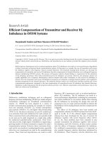
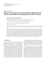
To explain in detail the path key establishment problem,
we illustrate using a small network having six sensor nodes
as shown in Figure 1. Solid and dashed lines are used to
represent physical and secure links, respectively. A secure link
exists if there is a shared secret between both end nodes. For
example, there is a secure link between node N
6
and node
N
1
, since they share a common key. On the other hand, node
N
6

and node N
4
have only a physical link since they do not
share a key. The following question arises: how could N
6
and
N
4
communicate?
A first solution is as follows: one node generates a
random key which can then be transmitted via a secure path
(N
6
-N
1
-N
5
-N
4
). The risk is that, if one node of this path is
captured, the key will be revealed. Thus, all communications
between the two nodes remain insecure. It has been proposed
in [9] to use multiple paths to send the generated key.
The new key will be divided according to the number of
secure paths between the two end sensor nodes. For example,
suppose there exist two secured paths between node N
6
and
node N
4

. The generated key will be divided into two parts
(nuggets). One part will be sent on the first path (N
1
-N
5
),
the other part will be sent via the second path (N
3
-N
2
). This
division obviously depends on the number of secure paths
that exist between them. The greater the number of paths, the
higher the chances of establishing a secure link. Therefore,
Noureddine Mehallegue et al. 3
an efficient algorithm for path key establishment problem
has to be employed taking into account the nature of WSNs
such as memory size and battery lifetime. Node Disjoint
Routing Protocol (NDRP), such as that described in [13], can
be used to find disjoint paths. Our work concentrates, not on
building node disjoint paths, but on how to elect proxies. The
proposed algorithm does not depend on a specific NDRP
algorithm.
Two methods have been proposed in [9] for the path
key establishment process. We use them as benchmarks for
assessing the performance of our proposed algorithm. The
algorithms in [9] are similar to the idea proposed by Liu et al.
in [6]. However, the new key is generated by one of the two
end nodes; while in [6], it is generated by a node which shares
a secret with both end nodes. In addition, these algorithms

use more than a single common node to send the new key
thereby giving added protection to the generated key.
2.1. Algorithm 1 (ALG1)
The basic steps of ALG1 to discover k proxies can be de-
scribed as follows [9].
(i) Node N
1
and node N
2
are two sensor nodes wishing to
set up a path to secure their communications.
(ii) Node N
1
randomly selects k neighbours (or (k − 1)
depending on whether or not node N
1
acts as its own
proxy for one key part or key nugget) and sends out
request for proxy packets containing key IDs for both
nodes N
1
and N
2
. Each recipient examines the key
identifiers (key IDs) list to determine if it shares keys
with both nodes N
1
and N
2
.

(a) If it does, it responds to node N
1
with the key ID
that is chosen to communicate with node N
1
.
(b) If it does not, or if it has received the same
request from node N
1
, it forwards this request to
a random neighbour, other than the sender.
2.2. Algorithm 2 (ALG2)
(i) Node N
1
creates a request packet and sets its time-
to-live (TTL) field to time interval t before locally
flooding the packet into the network. The value of t
may be set to reflect the density of the node within
the neighborhood. For dense networks, the value of
t should be small; while for sparse networks, a large
value of t may be required.
(ii) Nodes receiving a request packet respond with positive
acknowledgment only if they share a key with node N
1
and a key with node N
2
.
(iii) Upon receiving k positive acknowledgment, node N
1
selects the senders of these acknowledgments as k

proxies.
Both ALG1 and ALG2 include the case where nodes N
1
and
N
2
can act as their own proxies. The proxy process discovery
starts by looking for proxies either from node N
1
or node N
2
.
When a sensor node is elected as a proxy, the authors in [9]
do not assess the real length of the path between node N
1
and
node N
2
. For example, if this proxy is l
1
hops away from node
N
1
and l
2
hops away from node N
2
, then the real path will be
of length (l
1

+ l
2
). However, if node N
1
finds a proxy, which
is l
1
hops away, it is possible that this proxy shares a key with
node N
1
and node N
2
, but a path between this proxy and
node N
2
may not exist or be too far away.
In this paper, we propose a novel approach that elects
intermediate sensor nodes as proxies with a guaranteed short
path between the two end nodes.
3. PROPOSED ALGORITHM
The following assumptions are made in our algorithm
(ALG3) and its security analysis.
(1) Before the deployment phase, which is conducted
offline,
(a) each sensor node has a unique node identifier in
the network (node ID);
(b) each sensor node stores a list of keys or the
information necessary to set up a secure link
(DDHV scheme).
(2) After sensor deployment, the following occur.

(a) The key discovery phase takes place where each
node broadcasts its key IDs list. Therefore, each
node sends one message, and receives another
one from each node within its radio range.
Secure links are then set up at the end of the key
discovery phase.
(b) We assume that each sensor node has the sensor
node ID list of its first neighbours which have
a secure link with them (i.e., first neighbours).
The first neighbours of N
i
are defined as those
sensor nodes that are one hop away from a sensor
node N
i
and share a secret with node N
i
.Thus,
all communications between node N
i
and its
adjacent neighbours are secure.
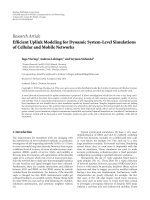
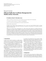
Let TIER (N
i
, j) denote the neighbours that are j hops away
from the node N
i
. Figure 2 illustrates the action of ALG3
where nodes N
1

and N
2
are two sensor nodes which are on
the radio range of each other. If nodes N
1
and N
2
wish to
establish a secure link, they exchange their key IDs’ list. If
they share a secret, they can set up a secure link.
Assume that nodes N
1
and N
2
do not share a secret. We
will show how ALG3 resolves the “Path Key Establishment
Problem.”
A physical link exists between nodes N
1
and N
2
,but
a secure path has yet to be established. ALG3 is initiated
after it is determined that no common secret exists between
nodes N
1
and N
2
.LetPrx denote the number of proxies
required to send the secret. Recall that node N

1
already
knows the ID list for its first neighbours (assumption 2(b)).
Then, node N
1
requests the sensor node ID list of node N
2
’s
first neighbours (those neighbours which are one hop away)
or node N
2
’s Tier 1 neighbours denoted by TIER(N
2
,1).
Then, N
1
starts comparing with its first neighbour sensor
node ID list, denoted as TIER(N
1
,1) (see CMP1 of Figure 2).
4 EURASIP Journal on Wireless Communications and Networking
TIER(N
1
,2)
TIER(N
1
,1)
TIER(N
2
,1)

TIER(N
2
,2)
N
1
N
2
CMP1
CMP2
CMP3
Request IDs list of TIER(N
2
,2)
Send IDs List of TIER(N
2
,2)
Request IDs list of TIER(N
1
,3)
Send IDs List of TIER(N
1
,3)
Request IDs list of TIER(N
2
,3)
Send IDs List of TIER(N
2
,3)
Request to set up
a secure link

Send Key
IDs List
No common Key
Request IDs list
of TIER(N
2
,1)
Send IDs List
of TIER(N
2
,1)
Request IDs list
of TIER(N
1
,2)
Send IDs list
of TIER(N
1
,2)
Figure 2: Proxy process discovery.
TIER(N
1
,1)
TIER(N
1
,2)
TIER(N
1
,3)
TIER(N

2
,1)
TIER(N
2
,2)
TIER(N
2
,3)
N
1
N
2
1
2
3
4
5
6
9
8
7
They cannot establish
a secure link
Figure 3: Chronological sequence comparison for proxy process
discovery.
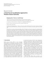
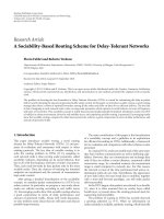
CMP1 corresponds to sequence 1 in Figure 3.Ifacommon
node ID is found, it will be elected as a proxy which is
one hop away from both end sensor nodes N
1
and N

2
(see
Figure 4(a)).
If the number of proxies found after CMP1 is smaller
than Prx,nodeN
1
continues searching for new proxies by
requesting the sensor node ID lists of its second neighbours
and node N
2
’s second neighbours by sending a request to its
first neighbours TIER(N
1
,1) and TIER(N
2
,1), respectively.
TIER(N
1
,1) replies by sending the sensor node ID
list of its first neighbours denoted by TIER(N
1
,2) (node
N
1
’s second neighbours). In addition, TIER(N
2
,1) replies
by sending the sensor node ID list of its first neigh-
bours denoted by TIER(N
2

,2) (node N
2
’s second neigh-
bours).
After receiving the required sensor node ID lists, node N
1
starts searching for new proxies by comparing at CMP2 the
sensor node ID list from its first and second neighbours with
node N
2
’s first and second neighbours (CMP2: see Figure 2).
CMP2 corresponds to sequences 2, 3, and 4 in Figure 3.The
chronological order of comparisons is depicted in Figure 3.
If new proxies are found, the length of the path will be as
follows (see Figure 4(b)):
(i) two, if the second neighbour of node N
1
is the first
neighbour of node N
2
or if the first neighbour of node
N
1
is the second neighbour of node N
2
;
(ii) three, if they both have a common second neighbour
ID.
If the required number of proxies found is smaller than
Prx,nodeN

1
requests its third neighbour sensor node
ID list and node N
2
’s third neighbours’ sensor node ID
list by sending requests to TIER(N
1
,2) and TIER(N
2
,2),
respectively. TIER(N
1
,2) replies by sending the sensor node
ID list of its first neighbours denoted by TIER(N
1
,3) (node
N
1
’s third neighbours) while TIER(N
2
,2) replies by sending
the sensor node ID list of its first neighbours denoted by
TIER(N
2
,3) (node N
2
’s third neighbours).
After receiving the sensor node ID list requested, node N
1
starts searching for new proxies by making comparisons at

Noureddine Mehallegue et al. 5
N
1
N
2
(a) Path length after
CMP1
N
1
N
2
(b) Path length after CMP2
N
1
N
2
(c) PathlengthafterCMP3
Figure 4: Path length after CMP1, CMP2, and CMP3.
CMP3 (see Figure 2). CMP3 corresponds to sequences 5, 6, 7,
8, and 9 in Figure 3. The chronological order of comparison
follows the sequence depicted in Figure 3.Ifproxiesare
found, the length of the path will be three, four, or five (see
Figure 4(c)).
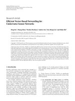
4. ANALYSIS
To assess the performance of our proposed algorithm, the
same experiment as described in [9, 14] with 1000 sensor
nodes randomly distributed over a 100
× 100 square area
was carried out. Simulations were run using Matlab [15].
Three different scenarios were simulated in which the radio

range R was set to 6, 8, and 12 in order to generate networks
with different densities. In Figure 5, when R
= 6, the sensor
node highlighted in black can attempt to establish a secure
link with up to six sensor nodes. When R
= 8andR = 12,
the number of sensor nodes that can be targeted to establish
secure links with increases.
In these experiments, a path key is fragmented into 5
parts (nuggets). Thus, five proxies are required to commu-
nicate the path key between two end nodes so that 100 pairs
of end nodes were chosen randomly in our simulations. The
performance of ALG3 was compared with both ALG1 and
ALG2 using different key distribution scenarios.
4.1. Average number of hops to find a proxy
Figures 6 and 7 show the average number of hops to deter-
mine one proxy in the network for two different scenarios
exhibiting low and high connectivity.
Figure 6 depicts the average number of hops to find one
proxy in a network with a 30% probability that any two nodes
share a secret. When R
= 6(i.e.,forasparsenetwork),a
proxy can be found after more than 9 hops and 3 hops using
ALG1 and ALG2, respectively. However, using ALG3, a proxy
resides fewer than two hops away. In [9], the authors did
not assess the path length l between nodes N
1
and N
2
.For

example, using ALG1, a proxy resides more than 9 hops away
from node N
1
for the case when R = 6. For this case, the
path length between node N
1
and node N
2
is at least 10 hops
if the elected proxy is a first neighbour of node N
2
.However,
this does not always happen. Using ALG2, the path length l
has 4 hops. In our simulations, a proxy is found almost after
exchanging the first, second, and third neighbours’ sensor
node ID list and resides one or two hops away from node
20
22
24
26
28
30
32
34
36
38
40
42
44
46

48
50
20 22 24 26 28 30 32 34 36 38 40 42 44 46 48 50
R
= 6
R
= 8
R
= 12
Figure 5: Varying radio range and connectivity.
N
1
such that the path length is 2 ≤ l ≤ 4 (see Figure 4).
For a medium dense network (R
= 8),aproxyis8hops
and 2 hops away when using ALG1 and ALG2, respectively.
When R
= 12 (i.e., for a dense network), one still needs more
than 8 hops and 2 hops using ALG1 and ALG2, respectively.
In this case, ALG3 outperforms both ALG1 and ALG2 since
a proxy resides less than 2 hops away from node N
1
(see
Figure 6).
Another feature of ALG3 is that it is independent of
the network density making it more appropriate for WSNs.
Figure 7 shows the average number of hops to locate one
proxy for another scenario where the probability that any
twosensornodesareabletocommunicateis60%.Itcan
be observed from Figures 6 and 7 that the number of hops

to determine one proxy in the case when R
= 6falls
from from 9 to 3 for ALG1 and from 3 to 2 for ALG2
when the probability that any two sensor nodes are able
to communicate is varied from 30% to 60%. Using ALG3,
the average number of hops to find one proxy is almost
“1.” This means that there is a higher chance of finding
a proxy residing one hop away from nodes N
1
and N
2
compared to the scenario in Figure 6. Using ALG3, the
degree of connectivity is not so influential as regards the
number of hops needed to find a proxy as in the case of
ALG1 and ALG2. This is an advantage in the case when the
connectivity of the network is reduced due to power or node
failures.
6 EURASIP Journal on Wireless Communications and Networking
0
1
2
3
4
5
6
7
8
9
10
Hops

R = 6 R = 8 R = 12
ALG1
ALG2
ALG3
Figure 6:Averagenumberofhopstogetoneproxyforascenario
with low connectivity (τ
= 4; ω = 50; P
actual
= 30%).
0
1
2
3
4
5
6
7
8
9
10
Hops
R = 6 R = 8 R = 12
ALG1
ALG2
ALG3
Figure 7:Averagenumberofhopstogetoneproxyforascenario
with high connectivity (τ
= 6; ω = 50; P
actual
= 60%).

4.2. Average time to find one proxy
To further demonstrate the superiority of the performance
of ALG3, we have recorded the average time necessary to
establish a secure link between two sensor nodes which does
not share a secure one. The time computed is the interval
between the request to set up a secure link and its final
establishment (see Figure 2). In order to simulate a real
scenario, the IEEE 802.15.4 standard is implemented to assess
our proposed algorithm. The frame sequence in 802.15.4
is depicted in Figure 8(a). One frame duration includes
theback-off period, the frame to be transmitted, turn-around
time, acknowledgment and the interframe space (IFS). It
has to be noticed that the long frames are followed by a
long IFS (LIFS) and short frames by a short IFS (SIFS).
More information on the 802.15.4 can be found in [16]. The
data frame (Figure 8(b)) structure and the medium access
control (MAC) command frame (Figure 8(c)) of 802.15.4
[16] protocol are used to to send the sensor node ID
list and request the establishment of a secure link, respec-
tively.
The following assumptions are considered while record-
ing the average time to determine a proxy.
(i) There are no losses due to collisions; no packets are lost
due to bufferoverflowateithersenderorreceiverside.
The bit error rate is zero. Therefore, a perfect channel
is considered in this study.
(ii) The unslotted version of the 802.15.4 protocol in
the 2.4 GHz band is implemented which provides the
highest data rate (250 Kb/s).
(iii) The short addressing mode is used.

(iv) Acknowledgment packets are omitted.
(v) The number of back-off slots is a random number
uniformly distributed in the interval [0, 2
BE
− 1], BE is
the back-off exponent which has the minimum value
of 3. As a perfect channel is considered with a BER
= 0,
the number of back-off slots can be represented as the
mean of the interval: [(2
3
− 1)/2] = 3.5.Thetimefor
aback-off slot is 320 μs.
(vi) SIFS is used when the MAC protocol data unit
(MPDU) is smaller than 18 bytes (SIFS
= 192 μs).
Otherwise, LIFS is used (LIFS
= 640 μs).
The time computed includes the passive listening of all the
nodes involved in the proxy searching process. When the
probability of sharing a secret is 30%, each sensor node
carries 20 keys randomly from a key pool of 1000. The
key ID identifiers require 10 bits to represent them in a
binary format. The Data payload for the request packet size
is 15 bytes. Therefore, each request packet transmitted is
followed by a SIFS (MPDU < 18 bytes). The data packet
size to send the key ID list is 59 bytes and 79 bytes when
P
actual
= 30% and P

actual
= 60%, respectively. In both
scenarios, each data packet transmitted is followed by a LIFS
(MPDU > 18 bytes). The request packet size is 21 bytes. Both
ALG1 and ALG2 compare the key ID lists to elect a proxy
(Section 2) whereas ALG3 compares the sensor node ID lists
(common trusted neighbours). When, the probability that
two sensor nodes are able to communicate is set to 30%,
each sensor node carries 20 keys. Thus, 20 comparisons are
required each time. Furthermore, the key IDs of both end
nodes need to be transmitted to each sensor node in order
for it to be elected as a proxy. This means higher-power
consumption.
Figure 9 clearly shows that the average active time to
transmit the necessary information to find one proxy using
ALG1 and ALG2 is much higher than ALG3 for a scenario
when P
actual
= 30% with a data rate of 250 Kb/s. When R = 6,
ALG1 and ALG2 require 527.2 ms and 216.4 ms, respectively,
to find one proxy whereas ALG3 requires only 61.85 ms. For
a medium dense network (R
= 8), ALG3 outperforms both
Noureddine Mehallegue et al. 7
Long Frame
ACK
Turnaroundtime
LIFS
Back Off Period
Short Frame

ACK
Turnaroundtime
SIFS
1 frame duration
(a) Frame sequence of 802.15.4 protocol
Octets: 2 1 4 to 20 n 2
Octets: 4 1 1 5 + (4 to 20) + n
11 + (4 to 20) + n
MAC
sublayer
Physical
layer
PPDU
Physical Protocol Data Unit
Frame
Control
Sequence
Number
Addressing
Fields
Data
Payload
FCS
Frame Check
Sequence
MHR
MAC Header
MSDU
MAC Service
Data Unit

MFR
MAC FooteR
Preamble
Sequence
Start of
Frame
Delimiter
Frame
Length
MPDU
MAC Protocol Data Unit
(b) Data frame structure of 802.15.4 protocol
Octets: 2 1 4 to 20 1 n 2
Octets: 4 1 1 6 + (4 to 20) + n
12 + (4 to 20) + n
MAC
sublayer
Physical
layer
PPDU
Physical Protocol Data Unit
Frame
Control
Sequence
Number
Addressing
Fields
Command
Type
Command

Payload
FCS
MHR MSDU MFR
Preamble
Sequence
Start of
Frame
Delimiter
Frame
Length
MPDU
MAC Protocol Data Unit
(c) MAC command frame structure of 802.15.4 protocol
Figure 8: IEEE 802.15.4 frame sequence, data, and command frame structure.
ALG1 and ALG2 (see Figure 9: R = 8). When R = 12 (i.e., for
a dense network), ALG3 requires less time than the others to
find one proxy (see Figure 9: R
= 12).
Figure 10 shows another scenario for the case when
the probability of any two sensor nodes being able to
communicate is set to 60%. In this scenario, each sensor
node carries 30 keys. Thus, 30 comparisons have to be made
each time. When R
= 6 (for a sparse network), Figure 10
shows that the average times to find one proxy using ALG1,
ALG2, and ALG3 are 80.42 ms; 118.73 ms, and 33.39 ms,
respectively. It can also be seen that, for a medium dense
network (R
= 8), ALG3 outperforms both ALG1 and ALG2.
Finally, for a dense network (R

= 12), ALG3 still performs
better than both ALG1 and ALG2. Thus, ALG3 outperforms
both ALG1 and ALG2 across the full range of network types.
4.3. Average time to find five proxies
Simulations to find five proxies have been made. The average
active times to determine the five proxies using ALG1, ALG2,
and ALG3 have been recorded. Figures 11 and 12 clearly show
that ALG3 outperforms both ALG1 and ALG2.
Figure 11 depicts the average time to determine the
five proxies for a network with a low connectivity (30%).
For a sparse network (R
= 6), ALG1, ALG2, and ALG3
require 2635.9 ms, 1082.1 ms, and 181.95 ms, respectively,
to find five proxies. For R
= 8, the average times to
determine five proxies using ALG1, ALG2, and ALG3 are
2344.9 ms, 773.3 ms, and 151.63 ms, respectively. Finally, for
a dense network (R
= 12), ALG1, ALG2, and ALG3 require
2178.5 ms, 685.5 ms, and 218.46 ms, respectively, to find five
8 EURASIP Journal on Wireless Communications and Networking
0
50
100
150
200
250
300
350
400

450
500
550
Time (ms)
R = 6 R = 8 R = 12
ALG1
ALG2
Our ALG
Figure 9: Average time to find one proxy with low connectivity
(data rate
= 250 Kb/s; P
actual
= 30%).
0
20
40
60
80
100
120
Time (ms)
R = 6 R = 8 R = 12
ALG1
ALG2
ALG3
Figure 10: Average time to find one proxy with high connectivity
(data rate
= 250 Kb/s; P
actual
= 60%).

proxies. Figure 12 shows another scenario when P
actual
is set
to 60% and the data rate is set to 250 Kb/s. It is observed that
ALG3 requires less time to find five proxies than do ALG1
and ALG2. For a sparse network (R
= 6), ALG1, ALG2,
and ALG3 require 402.08 ms, 593.65 ms, and 122.27 ms,
respectively,tofindfiveproxies.ForR
= 8, the average times
to determine five proxies using ALG1, ALG2, and ALG3 are
350.27 ms, 311.95 ms, and 121.11 ms, respectively, while for
a dense network (R
= 12), ALG1, ALG2, and ALG3 require
257.33 ms, 213.91 ms, and 123.41 ms, respectively, to find
five proxies. Thus, ALG3 outperforms both ALG1 and ALG2
across the full range of network types.
ALG3 optimises the time necessary to find common
nodes to send the new generated key which will be divided
according to the number of elected proxies. The time to
find those elected proxies using ALG1 and ALG2 is longer
0
500
1000
1500
2000
2500
3000
Time (ms)
R = 6 R = 8 R = 12

ALG1
ALG2
ALG3
Figure 11: Average time to find five proxies with low connectivity
(P
actual
= 30%; data rate = 250 Kb/s).
0
100
200
300
400
500
600
Time (ms)
R = 6 R = 8 R = 12
ALG1
ALG2
ALG3
Figure 12: Average time to find five proxies with high connectivity
(P
actual
= 60%; data rate = 250 Kb/s).
than ALG3. Both ALG1 and ALG2 elect a sensor node as
a proxy only if it has a common key ID with both end
sensor nodes N
1
and N
2
. For a probability of sharing one

key space of 30%, each sensor node carries 20 keys from
a key pool of 1000 keys. Therefore, each time a request to
establish a secure link is sent to a neighbouring node; a
total of two times 20 comparisons of keys ID are required
to be made to decide whether that node has a common key
with both nodes N
1
and N
2
. On the top of that, ALG1 and
ALG2 do not guarantee that a secure link exists between the
elected proxy and N
2
. Furthermore, the length of the path
between N
1
and N
2
is not considered in [9]. Our proposed
method searches proxies by comparing the sensor node ID
resulting in shorter paths and less time to establish a secure
link. Consequently, ALG3 is suitable for WSNs nature (see
Ta ble 1).
Noureddine Mehallegue et al. 9
Table 1: Comparison of ALG1, ALG2, and ALG3.
ALG1 ALG2 ALG3
Resolve the path key establishment problem for WSNs
Suitable for sparse WSNs Suitable for dense WSNs Suitable for WSNs
The elected proxies are far away resulting
Thepathlengthisshorterthan

in a higher path length between N
1
and N
2
.
both ALG1 and ALG2.
It takes both ALG1 and ALG2 a longer time to elect a proxy.
ALG3 requires less time to
The time is directly related to power consumption. Therefore,
elect a proxy. Therefore,
both ALG1 and ALG2 consume more power than ALG3.
it is more suited for WSNs.
5. CONCLUSION
This paper addresses the path key establishment problem
when two neighbouring sensor nodes with an insecure
link require their trusted neighbours to create a secure
link. The proposed algorithm outperforms two previously
developed algorithms [9]. The results and analyses relate to
scenarios for a WSN having high and low connectivities.
In particular, ALG3 can locate proxies with less difficulty
than those algorithms requiring shorter paths and showing
good performance for sparse wireless sensor networks (see
Figure 6).
In addition, it has been shown, through simulations, that
the proposed algorithm is more efficient in terms of the
active time to transmit the necessary information to find one
proxy and five proxies (see Ta ble 1). The time to determine a
proxy is directly related to power consumption, a longer time
necessarytoelectaproxywillresultinanextrapowertobe
consumed. Therefore the proposed algorithm is also power-

efficient. This demonstrates that the proposed algorithm is
well suited for use in wireless sensors networks.
REFERENCES
[1] I. F. Akyildiz, W. Su, Y. Sankarasubramaniam, and E. Cayirci,
“A survey on sensor networks,” IEEE Communications Maga-
zine, vol. 40, no. 8, pp. 102–114, 2002.
[2] C. Karlof and D. Wagner, “Secure routing in wireless sensor
networks: attacks and countermeasures,” in Proceedings of the
1st IEEE International Workshop on Sensor Network Protocols
and Applications (SNPA ’03), pp. 113–127, Anchorage, Alaska,
USA, May 2003.
[3] L. Eschenauer and V. D. Gligor, “A key management scheme
for distributed sensor networks,” in Proceedings of the 9th
ACM Conference on Computer and Communication Security
(CCS ’02), pp. 41–47, Washingtion, DC, USA, November
2002.
[4] H. Chan, A. Perrig, and D. Song, “Random key predistribution
schemes for sensor networks,” in Proceedings of IEEE Sym-
posium on Security and Privacy, pp. 197–213, Oakland, Calif,
USA, May 2003.
[5] W. Du, J. Deng, Y. S. Han, P. Varshney, J. Katz, and A. Khalili,
“A pairwise key predistribution scheme for wireless sensor
networks,” ACM Transactions on Information and System
Securit y, vol. 8, no. 2, pp. 228–258, 2005.
[6] D. Liu, P. Ning, and R. Li, “Establishing pairwise keys in dis-
tributed sensor networks,” ACM Transactions on Information
and System Security, vol. 8, no. 1, pp. 41–77, 2005.
[7] R. Blom, “An optimal class of symmetric key generation
systems,” in Proceedings of the Workshop on the Theory and
Application of Cryptographic Techniques (EUROCRYPT ’84),

pp. 335–338, Paris, France, April 1985.
[8] N. Mehallegue, E. Garcia, and A. Bouridane, “Improving key
distribution for wireless sensor networks,” in Proceedings of the
2nd IEEE NASA/ESA Conference on Adaptive Hardware and
Systems, pp. 82–88, Edinburgh, Scotland, UK, August 2007.
[9] G. Li, H. Ling, T. Znati, and W. Wu, “A robust on-demand
path-key establishment framework via random key predis-
tribution for wireless sensor networks,” EURASIP Journal on
Wireless Communications and Networking, vol. 2006, Article
ID 91304, 10 pages, 2006.
[10] R. Anderson, H. Chan, and A. Perrig, “Key infection: smart
trust for smart dust,” in Proceedings of the 12th IEEE Interna-
tional Conference on Network Protocols (ICNP ’04), pp. 206–
215, Berlin, Germany, October 2004.
[11] H. Chan and A. Perrig, “PIKE: peer intermediaries for key
establishment in sensor networks,” in Proceedings of the
24th Annual Joint Conference of the IEEE Computer and
Communications Societies (INFOCOM ’05), vol. 1, pp. 524–
535, Miami, Fla, USA, March 2005.
[12] S. Zhu, S. Xu, S. Setia, and S. Jajodia, “Establishing pairwise
keys for secure communication in ad hoc networks: a proba-
bilistic approach,” in Proceedings of the 11th IEEE International
Conference on Network Protocols (ICNP ’03), pp. 326–335,
Atlanta, Ga, USA, Novemeber 2003.
[13] X. Li and L. Cuthbert, “Node-disjointness-based multipath
routing for mobile ad hoc networks,” in Proceedings of the
1st ACM Inter n ational Workshop on Performance Evaluation
of Wireless Ad Hoc, Sensor, and Ubiquitous Networks (PE-
WASUN ’04), pp. 23–29, Venice, Italy, October 2004.
[14] H. Ling and T. Znati, “End-to-end pairwise key estab-

lishment using multi-path in wireless sensor network,” in
Proceedings of IEEE Global Telecommunications Conference
(GLOBECOM ’05), vol. 3, pp. 1847–1851, Saint Louis, Mo,
USA, November-December 2005.
[15] www.mathworks.com/.
[16] IEEE Std. 802.15.4, “IEEE standard for Information
Technology—Telecommunications and information exchange
between systems—Local and metropolitan area networks—
Specific requirements, Part 15.4 Wireless Medium Access
Control (MAC) and Physical Layer (PHY) Specifications for
Low Rate Wireless Personal Area Networks (LR-WPANs),”
IEEE Computer Society, September 2006.