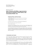
Báo cáo hóa học: "Research Article Fuzzy Mode Enhancement and Detection for Color Image Segmentation" docx

Hindawi Publishing Corporation
EURASIP Journal on Image and Video Processing
Volume 2008, Article ID 542378, 19 pages
doi:10.1155/2008/542378

Research Article
Fuzzy Mode Enhancement and Detection for
Color Image Segmentation
Olivier Losson, Claudine Botte-Lecocq, and Ludovic Macaire
Laboratoire LAGIS (CNRS UMR 8146), Universit´ des Sciences et Technologies de Lille, Bˆ timent P2, Cit´ Scientifique,
e
a
e
59655 Villeneuve d’Ascq C´dex, France
e
Correspondence should be addressed to Olivier Losson,
Received 20 July 2007; Revised 30 November 2007; Accepted 27 January 2008
Recommended by Konstantinos Plataniotis
This work lies within the scope of color image segmentation by pixel classification. The classes of pixels are constructed by detecting
the modes of the spatial-color compactness function, which characterizes the image by taking into account both the distribution
of colors in the color space and their spatial location in the image plane. A fuzzy transformation of this function is performed,
based on fuzzy morphological operators specifically designed for mode detection. Experimental segmentation results, using several
synthetic and benchmark images, show the interest of the proposed method.
Copyright © 2008 Olivier Losson et al. This is an open access article distributed under the Creative Commons Attribution License,
which permits unrestricted use, distribution, and reproduction in any medium, provided the original work is properly cited.

1.

INTRODUCTION

Color image segmentation consists in partitioning the pixels of an image into separate regions, which are groups

of connected pixels with homogeneous color properties.
Among low-level image processing tasks, segmentation is
one of the most challenging and addressed issues. Indeed,
this step is crucial in many applications requiring region
and object identification in the scene, as in content-based
image retrieval schemes, object-based video coding, and so
on. Color image segmentation is classically achieved by an
analysis of either the image plane or a color space.
Image plane analysis methods can be divided into two
major categories. The boundary-based methods look for
discontinuities in the image to detect edge pixels [1, 2]. They
often require time-consuming postprocessing tasks, such as
edge tracking, to yield closed object boundaries. Conversely,
region-based techniques assume that neighboring pixels
belonging to the same region share similar color properties.
Region growing procedures start from selected seed pixels
and iteratively aggregate all similar neighbors that respect
homogeneity-based conditions [3]. They generally result in
an oversegmented image, which can be processed by region
merging algorithms. These algorithms usually model the
image by a region adjacency graph, and then analyze such

a graph in order to iteratively merge adjacent regions with
similar colors [4].
Since most of the image plane analysis methods require a
delicate adjustment of parameters, a lot of authors propose
to globally analyze the color distribution in a color space
by means of pixel classification techniques. For this purpose,
each pixel is associated with a color point whose coordinates
are its color component levels (e.g., red, green, and blue levels

when the (R, G, B) color space is considered).
Image segmentation methods by pixel classification rely
on the assumption that homogeneous regions in the image
give rise to clusters of color points in the color space, each
of them corresponding to a class of pixels. The key problem
consists in cluster identification, based on either a clustering
technique or an analysis of an underlying probability density
function (pdf).
Clustering schemes aim at identifying the gravity centers
of clusters thanks to dedicated metrics in the color space
[5], such as the Euclidean distance used by a competitive
learning scheme [6] or a fuzzy metric used by the fuzzy Cmeans method [7]. Consequently, most of these schemes
make strong assumptions about the cluster shapes. When
the distributions of the color points are neither globular
nor compact, these clustering techniques tend to fail in
constructing pixel classes which correspond to the actual
regions in the image.


2
In order to avoid this problem, several authors propose
to analyze the underlying pdf of all the colors occurring in
the image. This function can be directly approximated by
the 3D color histogram. Each bin, whose coordinates in the
histogram are the component levels of a given color, is valued
with the number of pixels having the corresponding color in
the image. Cluster identification is achieved by detecting the
domains of the color space with a high density of points (i.e.,
the domains—called modes—where the pdf reaches high
values). The pixels whose colors are located in these modes

define the prototypes of the classes. The remaining unlabeled
pixels are finally assigned to one of these classes according
to a decision rule. In that way, the constructed regions of
the segmented image are composed of the connected pixels
assigned to the same classes.
As far as color image segmentation is primarily viewed
as a mode detection problem, local maximums of the pdf
may be seen as peaks, whereas low values of the pdf may be
considered as valleys. This topographic point of view enables
to exploit techniques such as watershed-based methods
[8]. Originally applied to a gradient image, the algorithm
using immersion [9] has been run on the additive inverse
histogram [10]. Nonetheless, it still provides oversegmented
images and therefore requires a mode merging step [11],
even in user-assisted schemes [12]. Hill climbing has also
been investigated, but this approach is subject to loss of
details. Therefore, it requires histogram peak manipulations
to avoid that small yet significant peaks get merged with
larger ones [13].
Zhang et al. propose to detect valleys of the pdf, instead
of modes, by examining the normalized density derivative of
the pdf [14]. The underlying hypothesis is that there is no
abrupt change in density between two adjacent colors that
belong to the same mode. A final convexity test is performed
to improve the robustness of the procedure when the color
distributions highly overlap in the color space.
Most of pixel classification schemes are designed to
identify either globular or ellipsoidal clusters of color points,
or modes which are well separated by valleys of the pdf.
Unfortunately, those strong assumptions are not always

verified, especially for real noisy natural images when the
objects of the observed scene are illuminated with a spatially
nonuniform lighting. That explains why a lot of color
image segmentation methods by pixel classification fail in
distinguishing the objects when the lighting intensity varies
all over the scene. The issue tackled here is related to the
construction of pixel classes thanks to mode detection when
the color distributions of the distinct regions to be retrieved
are nonglobular.
In Section 2, we focus on the specific problem of
color image segmentation in case of nonuniform lighting.
In Section 3, we introduce the spatial-color compactness
function characterizing a color image. Then, we detail the
key point of this paper, namely how to detect the modes
of this function by means of a specific fuzzy morphological
transformation in Section 4. Experimental results are provided in Section 5 in order to assess the effectiveness of our
fuzzy mode detection scheme for color image segmentation.
Finally, a conclusion is made in Section 6.

EURASIP Journal on Image and Video Processing
2.
2.1.

IMAGE SEGMENTATION AND
NONUNIFORM LIGHTING
Illustrative example

Let us consider the simple case of a scene composed of two
distinct one-colored objects, the reflectance properties of
each object being identical all over its surface. So, when the

surface of each object is illuminated by a uniform lighting,
the colors of pixels representing it are identical. Because of
the Gaussian acquisition noise, colors give rise to clusters
which, depending on their overlapping degree, can be more
or less easily identified by clustering methods designed for
image segmentation.
When the lighting intensity gradually varies all over the
object surface, the (R, G, B) color components of the pixels
vary too. As an example, the synthetic image in Figure 1(a) is
made of two rectangular surfaces illuminated by a lighting
whose intensity increases with respect to the pixel row
coordinates. In order to simplify the illustration, the blue
component has been set to zero all over the image, as for all
the synthetic images used in this paper. Figure 1(b) shows the
histogram H(R, G) of this image where R and G are the color
components of each pixel. Since the reflectance properties are
identical all over the surface of each object and since there is
no acquisition noise, the colors of the two surfaces give rise
to two diagonal linear modes of the histogram in the (R, G)
chromatic plane.
In order to take into account the acquisition noise, this
image is corrupted by a noncorrelated Gaussian noise, with
a standard deviation equal to 10, which is independently
added to each color component (see noisy synthetic image in
Figure 2(a)). Figure 2(b) shows that, since the distributions
of these colors highly overlap, the two modes are not well
separated by a valley. Therefore, they are hardly detectable by
an automatic processing of this histogram. This is essentially
due to the fact that the histogram only considers the colors
of the pixels and ignores their spatial location in the image.

So, in case of nonuniform lighting, the histogram is not
always a relevant tool for color image segmentation by mode
detection.
2.2.

Spatial-color pixel classification

Spatial-color pixel classification approaches take into
account both the distribution and the spatial location of the
colors to segment the image. This family of recent methods
can be divided into two groups: the techniques which apply a
clustering procedure followed by a spatial analysis, and those
which detect the modes by analyzing spatial-color functions
describing the image.
Ye et al. apply the clustering algorithm called DBSCAN
to image segmentation [15]. First, this scheme identifies core
pixels, namely pixels surrounded by a minimum number of
neighbors with similar colors. The similarity is ensured if
the colors of the considered pixels are located in an ellipsoid
of the (H, V , C) color space. Then, the procedure regroups
pixels which are density-reachable from those detected core
pixels.


Olivier Losson et al.

3

H (R, G)

0

10
5
0

50
100

0
50

150

100
G

150

R

200

200
250

(b) Histogram in the (R, G) plane

(a) Synthetic image

Figure 1: Synthetic image of two surfaces illuminated by a spatially nonuniform lighting intensity.

H (R, G)

0

9
50

0
100

0
50

150

100
G

150

R

200

200
250

(a) Noisy synthetic image

(b) Histogram in the (R, G) plane

Figure 2: Synthetic image, corrupted by acquisition noise, of two surfaces illuminated by a spatially nonuniform lighting intensity.

JSEG is one of the most well-known segmentation
algorithms which achieve a clustering step followed by a
spatial analysis [16]. A first step of color quantization yields
an image of labels called class-map. Considering the classmap as a special color-texture composition, the proposed
J measure relies on the dispersion of the locations of
the prototype pixels to provide a “good” segmentation
criterion. The local homogeneity measure J, computed on
a neighborhood of a given size, is all the higher as the
center pixel likely belongs to a region boundary. Using the
J criterion, a region merging procedure is finally applied
to the class-map in order to avoid oversegmentation. Wang
et al. [17] show that the hard classification caused by
the color quantization step both degrades the flexibility of
JSEG and, subsequently, tends to split the image areas with
smooth color transitions into several classes. Figure 3(a),
which shows the JSEG segmentation of the synthetic image in
Figure 2(a), illustrates this phenomenon. In this image, as in
the following segmented ones, the edges of the reconstructed
regions are white marked. This segmentation result is
provided by the software implementing JSEG, available on
the web site />
and configured with the default parameter values suggested
by the authors. Wang et al. argue and illustrate on a simple
example that the J measure, being applied to a class-map,
fails to give the boundary strength and hence does not

allow to distinguish regions with similar distributions of
textural patterns but different color contrasts [18]. JSEG
is therefore prone to oversegmentation in case of spatially
varying lighting. Those authors ascribe it primarily to the
fact that color and spatial information are taken into account
separately. Therefore, they propose to combine the textural
homogeneity measure J and the color discontinuity measure
H used by HSEG method [19]. This combined measure is
suitable to characterize homogeneous texture regions, and
to make distinguishable class-maps with strong and weak
boundaries.
Comaniciu and Meer construct a spatial-color function
describing the image, and propose to detect the modes by
jointly considering spatial and color distributions. They
apply the mean shift algorithm in the joint spatial-color space
for color image segmentation [20]. The mean shift method
is based on a kernel K, used by the Parzen density estimator,
and on a second kernel G defined from the derivative of the


4

EURASIP Journal on Image and Video Processing

(a) JSEG [16]

(b) Mean shift [20]

(c) SCDA [21]

Figure 3: Segmentation results of the image in Figure 2(a) provided by well-known spatial-color pixel classification methods.

profile function of K. At a given point, the mean shift is
computed as the difference between the weighted average of
the neighboring observations (using G as weights), and the
kernel center. For a set of points, the mean shift procedure
converges towards the maximums of the underlying pdf
without estimating the density. Moreover, the translation of
the kernel is automatically adapted to the local density of
points: low densities yield large mean shift steps. Once the
stationary points have been detected in this way, a pruning
procedure is necessary to retain only the local maximums
and hence to retrieve the modes. After nearby modes have
been pruned, each pixel is associated with a significant mode
of this joint space. As shown by Figure 3(b), the EDISON
software implementing the mean shift algorithm available at
/>and run with the default parameter values suggested by the
authors, provides oversegmentation in case of nonuniform
lighting.
Macaire et al. [21] also integrate both color distribution
and spatial location to construct the pixel classes. The
selection of color domains relies on the analysis of the spatialcolor compactness degree, which takes into account both
pixel connectedness and color homogeneity. This method
unfortunately requires the desired number of classes. Since it
assumes globular clusters of color points, it is inappropriate
for the identification of clusters with irregular shapes. As an
illustration of the limits reached by this approach, hereafter
referred to as SCDA, Figure 3(c) shows the corresponding
segmentation result obtained when the lighting is not
spatially uniform.

2.3. Our spatial-color approach
In this paper, we propose a new mode detection technique
based on the analysis of the spatial-color compactness function
(sccf) describing the color image. This function, called
compacigram in [22], describes both the distribution of the
colors in the color space and their spatial location in the
image plane. It is a trivariate function whose value at each
color point is a measure of the spatial-color compactness
degree, introduced by Macaire et al. [21] and described
in the next section. The modes to be detected are then
defined as color space domains where the sccf reaches

high values. They are separated by valleys, which are color
space domains where the sccf has low values. A first basic
mode detection procedure using convexity analysis has
been applied to the sccf in order to show the interest of
this describing function [22]. Nevertheless, the results of
such a procedure strongly depend on the thresholds used
to detect the modes. Moreover, a postprocessing step is
required to preserve only the significant detected modes. In
order to avoid these adjustments, we propose to perform
a fuzzy morphological transformation of the sccf based on
fuzzy morphological operators specially designed for mode
detection (see Section 4).
3.

SPATIAL-COLOR COMPACTNESS
FUNCTION OF A COLOR IMAGE

A color image can be described by the spatial-color compactness function sccf, which combines the connectedness and

homogeneity degrees, both introduced in [21] and briefly
described in the next subsection.
3.1.

Connectedness and homogeneity degrees

Let C = [CR , CG , CB ]T be a color point in the discrete color
space C = (R, G, B), and let Dl (C) be a cube, centered at
C and whose edges of length l (an odd integer) are parallel
to the axes of C. The cube Dl (C) therefore includes all the
color points C = [CR , CG , CB ]T adjacent to C, such that Ci −
(l − 1)/2 ≤ Ci ≤ Ci + (l − 1)/2, i = R, G, B. Let us consider
the color image I where each pixel P is characterized by its
color I(P). The subset formed by all the pixels P whose colors
I(P) are included in the cube Dl (C) is hereafter referred to as
Sl (C).
For any color point C of the color space, the connectedness degree CDl (C) is defined as the average number of
neighbors of each pixel of Sl (C) which also belong to Sl (C)
[23]. When the pixel subset Sl (C) is empty, CDl (C) is set to
0. Otherwise, by considering an nb × nb neighborhood of
each pixel (nb being an odd integer, set to 3 in this paper),
CDl (C) is defined as
CDl (C) =

P ∈Sl (C) Card N[Sl (C)](P)
nb2 − 1 ·Card Sl (C)

,

(1)

Olivier Losson et al.

5

where N[Sl (C)](P) is the subset of the neighboring pixels of
a pixel P ∈ Sl (C), among its (nb2 − 1) neighbors, which also
belong to Sl (C). This degree ranges from 0 to 1, and a value
of CDl (C) close to 0 indicates that the pixels of Sl (C) are
scattered in the image plane, while a value close to 1 means
that most of the pixels belonging to the considered subset are
connected to each other in the image.
The homogeneity degree HDl (C) is defined as the ratio of
the average local dispersion of colors in the neighborhood of
each pixel in Sl (C), to the global color dispersion of the pixels
belonging to Sl (C). The global dispersion measure, denoted
by σ(Sl (C)), is estimated as
σ Sl (C) =

1
Card Sl (C)
·

I(P) − I Sl (C)

T

I(P) − I Sl (C) ,

P ∈Sl (C)

(2)
where I(P) is the color of the pixel P in the image I, and
I(Sl (C)) is the mean color of the pixels which belong to Sl (C):
I Sl (C) =

1
I(P).
·
Card Sl (C) P∈Sl (C)

(3)

The local color dispersion measure of the subset Sl (C)
is defined as the mean of the color dispersion measures
σ(N[Sl (C)](P)) of the subsets N[Sl (C)](P) of all the pixels
P in Sl (C):
σlocal Sl (C) =

1
σ N Sl (C) (P) .
·
Card Sl (C) P∈Sl (C)

(4)

Note that the above local color dispersion at each pixel
in the subset Sl (C) only takes into account the colors of its
neighbors that also belong to Sl (C).

The homogeneity degree HDl (C) is then defined as
⎧
⎪ σlocal Sl (C)
⎨

HDl (C) = ⎪ σ Sl (C)
⎩
1,

,

if σ Sl (C) =0,
/

(5)

otherwise.

When the color points corresponding to the pixels in the
subset Sl (C) give rise to a compact cluster in the color space,
the homogeneity degree computed at C is close to 1. On
the opposite, when those color points form several distinct
clusters, the homogeneity degree is close to 0.
3.2. Spatial-color compactness function
The spatial-color compactness function (sccf) is a trivariate
function whose value at each color point C is defined as the
product of its connectedness and homogeneity degrees:
sccf(C) = CDl (C)·HDl (C),

(6)

where the edge length l of the cube Dl , used to process the
degrees all over the color space, is adjusted by the analyst. A
high value of sccf(C) indicates that the pixels in the subset

Sl (C) are highly connected in the image (CDl (C) close to
1) and that the color points corresponding to these pixels
are concentrated in the color space (HDl (C) close to 1).
Conversely, a low value of sccf(C) means that the pixels in
the subset Sl (C) are scattered in the image (CDl (C) close to
0) and/or that the color points of these pixels do not form a
distinct compact cluster in the color space (HDl (C) close to
0).
Figure 4(a) shows the sccf of synthetic image in
Figure 2(a), computed with the length l set to 7 in order to
ensure that the pixel subsets Sl (C) are populated enough. Let
us consider three different color points of the color space,
respectively, C1 , C2 , and C3 , highlighted as color patches on
this figure. We can see that the sccf values are high for both
C1 and C3 color points, since most of the pixels of the subsets
Sl (C1 ) and Sl (C3 ) are connected to each other in the image,
and since their colors are close together (see Figures 4(b) and
4(d)). Note that these two color points are located in the
two modes to be detected. On the opposite, at color point
C2 located in the main valley, the sccf value is low since the
pixels of the subset Sl (C2 ) are scattered in the image (see
Figure 4(c)). It is noticeable that the sccf highlights these two
modes which were not so obviously distinguishable on the
histogram of Figure 2(b).
4.

4.1.

MODE DETECTION BY A FUZZY MORPHOLOGICAL
TRANSFORMATION OF THE sccf
Introduction

Basic binary morphological tools have proved to be suited
for object segmentation [24] and for nonglobular mode
detection [25]. Park has proposed to detect the modes by
applying an adaptive dilation to the closing of the binary 3D
histogram, provided by thresholding the difference between
two Gaussian smoothed 3D histograms [26]. The aim of this
adaptive dilation scheme is to make two adjacent modes meet
each other at the valleys of the binary 3D histogram, while
preventing the modes to expand towards empty bins. If two
adjacent modes meet during dilation, the process is stopped
in the direction in which they tend to merge. The process
is completed either after a prespecified maximum number
of iteration steps or when no mode can be dilated any
more. The results depend both on the size of the structuring
element used by morphological operators, and on the choice
of the color space.
Multivalued morphological operators have also been
used to improve mode detection [27, 28]. Shafarenko has
proposed to apply the watershed algorithm to the chromaticity 2D histogram coded in the CIE (u∗ , v∗ ) chromatic
plane [29]. The acquisition noise is first reduced thanks
to a Gaussian filtering. The smoothed histogram is then
analyzed by the watershed algorithm in order to detect the
modes which correspond to the pixel classes. Xue et al.
consider three smoothed 2D histograms which represent

the color distribution projected on the (R, G), (R, B), and
(G, B) chromatic planes [11]. The watershed algorithm is
first applied to each of the three smoothed 2D histograms
in order to identify the modes in each chromatic plane, and


6

EURASIP Journal on Image and Video Processing
sccf (C1 ) = 0.05
C1 = [85, 78, 0]

sccf (C)

sccf (C2 ) = 0.01
C2 = [107, 127, 0]

0.15
0.1
0.05
0
0

0
50
100
50

150

100
C3 = [124, 163, 0]
sccf (C3 ) = 0.05

150
G

R

200

200
250

250

(a) Spatial-color compactness function (l = 7)

(b) Pixel subset Sl (C1 )

(c) Pixel subset Sl (C2 )

(d) Pixel subset Sl (C3 )

Figure 4: Spatial-color compactness function of the synthetic image in Figure 2(a), with three different color points and their corresponding
pixel subsets.

then to yield the three different corresponding segmented
images. In the last stage, these images are combined by
means of a region split and merge process, using the spatial

information from the 2D segmentations for the splitting
step while taking into account the color coded in the CIE
(L∗ , a∗ , b∗ ) space during the merging step.
The quality of segmentation results provided by these
methods strongly depends on the quality of mode detection.
Since only the color distribution is represented by the color
histogram, it is challenging to detect the modes which
correspond to the actual pixel classes to be retrieved. That is
the reason why we choose the sccf as the describing function
of the image.
4.2. From the sccf to the fuzzy set “mode”
As described in the previous section, the color points at
which the sccf reaches high values are likely to belong to the
modes associated with the pixel classes to be constructed. On
the opposite, the color points at which the sccf values are low
are located in the valleys and do not stand a chance to belong
to any mode.
Therefore, we propose to normalize the sccf in order to
compute the degree with which each color point C belongs
to a mode. In other words, the normalized sccf evaluates the
confidence degree in the statement “C belongs to a detected
mode associated with a pixel class”, and can be considered as

a mode membership function μM characterizing the fuzzy set
“Mode” denoted M and defined on the color space C:
∀C ∈ C,

μM (C) =

sccf(C)

.
maxC ∈C sccf(C )

(7)

High values of μM (close to 1) correspond to color points
C belonging to the modes, while low values (close to 0) are
associated with color points lying in the valleys between the
modes.
As it can be seen on the example of Figure 5, the mode
membership function associated with the sccf of Figure 4(a)
exhibits many irregularities, which makes the direct detection of the modes a tough task. In order to facilitate this
detection, we propose to perform a transformation of the
fuzzy set “mode” M, that is, a transformation of the mode
membership function μM , in order to enhance the modes
while enlarging the valleys.
Mathematical morphology is a set theory which provides
tools capable of such effects. Indeed, the most basic morphological operators, erosion, and dilation are often combined
in pair to result in the opening, wellknown for its filtering
properties [30]. The main effect of erosion is to enlarge the
valleys by eliminating the irregularities of the distribution,
but this operation also tends to shrink the modes. On the
other hand, dilation is used to enhance the modes, but it also
tends to fill the valleys [8].


Olivier Losson et al.

7
As an illustration, let us consider the mode membership

function μM of Figure 5, and the binary structuring function
γ defined as

μM (C)

γ d∞ (C, C ) =
1

1,
0,

if C ∈ Ds (C),
otherwise.

(9)

0

0.5

50

0
0

100
50

150

100
150
G

R

200

200
250

250

Figure 5: Mode membership function of the synthetic image in
Figure 2(a).

The eroded and dilated membership functions Eγ [μM ]
and Dγ [μM ] are presented in Figures 6(a) and 6(b), respectively, s being set to the same value as the cube edge length
l used to compute the sccf. This example shows that the
classical fuzzy erosion tends to enlarge the valleys while
shrinking the modes, whereas the classical fuzzy dilation
tends to enlarge the modes while filling the valleys.
4.4.

We propose to transform the fuzzy set “mode” M, and
therefore its associated mode membership function μM ,
by means of fuzzy morphological operators which aim at
increasing the contrast between modes and valleys. The
key point is to exploit the advantages of these two basic
operations of erosion and dilation while avoiding their

drawbacks. Such an idea has already been explored in [31],
where the mode membership function is extracted thanks
to a fuzzification step involving a convexity analysis of the
color histogram. However, this method needs the adjustment
of many parameters and its success highly depends on the
result of the histogram fuzzification step. Moreover, since the
membership function introduced in [31] ignores the spatial
location of the colors in the image plane, the pixel classes
associated with the detected modes may not correspond to
the actual regions in the image. So, in this paper, we propose
to apply these interesting fuzzy morphological operators to
the mode membership function, derived from the sccf, in
order to detect the modes.
4.3. Classical fuzzy erosion and dilation operators
The selected classical fuzzy erosion and dilation operators
are those which generate the strongest effects of erosion and
dilation [32]. They use a fuzzy structuring element defined
by its cube Ds of edge length s and by its membership
function γ called the structuring function.
In this way, the selected fuzzy erosion Eγ and fuzzy
dilation Dγ operators, applied to the mode membership
function μM at a color point C, are defined in the literature
as
Eγ μM (C) = min

max μM (C ), 1 − γ d∞ (C, C )) ,

Dγ μM (C) = max

min μM (C ), γ(d∞ (C, C )) .

C ∈Ds (C)
C ∈Ds (C)

Fuzzy erosion and dilation operators specifically
designed for mode detection

4.4.1. Fuzzy operators
In order to facilitate the detection of the modes, it would be
pertinent to define a fuzzy erosion operator which enlarges
the valleys without shrinking the modes, and a fuzzy dilation
operator which enhances the modes without filling the
valleys. To be more specific, if a color point C is close to a
mode, it is relevant to strengthen the dilation effect at the
location of this color point C and to limit the erosion effect in
order to preserve that mode. Moreover, this color point more
likely belongs to this mode when its adjacent color points C
are also close to the same mode. Conversely, if the color point
C is far from all modes, it is probably located in a valley. In
this case, it is useful to erode the mode membership function
at the location of this color point without dilating it. Such a
color point is all the more likely located within a valley than
its adjacent color points are also located within a valley. This
implies to erode or dilate the mode membership function
more or less, depending on the location of each color point
in the color space and on its adjacent color points.
In the classical definitions of the fuzzy operators
described by (8), the structuring function γ depends on the
infinity norm distance between the considered color point
C and each of its adjacent color points C , but does not

depend on their mode membership degrees. However, if the
mode membership degree of an adjacent color point is high,
it would be interesting to take it into account only for the
dilation, but not for the erosion. On the other hand, if the
membership degree of an adjacent color point is low, its
contribution should be stronger for the erosion than for the
dilation. This means that both the fuzzy erosion and dilation
operators should be defined by their own specific structuring
functions:
EγE μM (C) = min

C ∈Ds (C)

max μM (C ), 1 − γE (C ) ,
(10)

(8)
The structuring function γ used by the erosion and
dilation operators depends on the infinity norm distance
d∞ (C, C ) = max(|CR − CR |, |CG − CG |, |CB − CB |) between
C and any of its adjacent color points C in Ds (C).

DγD μM (C) = max

C ∈Ds (C)

min μM (C ), γD (C ) ,

(11)

with γE and γD being described in Sections 4.4.2 and 4.4.3,
respectively.


8

EURASIP Journal on Image and Video Processing

Dγ [μM (C)]

Eγ [μM (C)]

1

1

0

0.5

50

0
0
150

100
150

100

50

R

250

150

100
150

200

200

G

50

0
0

100
50

0

0.5

(a) Classical fuzzy erosion

200

200

G

250

R

250

250

(b) Classical fuzzy dilation

Figure 6: Results of the classical fuzzy morphological operations applied to the mode membership function of Figure 5 (s = 7).

4.4.2. Specific structuring function associated with
the fuzzy erosion

as

The fuzzy erosion, expressed by (10), is performed using
a specific structuring function γE defined for each of the
adjacent color points C in the structuring element cube
Ds (C). We propose to define this structuring function γE as
⎧
⎨1,

γE (C ) = ⎩

if fM (C ) ≤ f M ,

μM (C),

otherwise,

(12)

where fM is a decision function and f M the mean value of
this function (see (13), (14), and (15)).
The decision function fM is defined according to the
following assumption: in the color space, an adjacent color
point C (included in the cube Ds (C)) can be located in
a mode, in a valley, or in the border between the two. An
adjacent color point C , which is close to the border between
a valley and a mode, is characterized by significant local
variations between its mode membership degree and the
mode membership degrees of its adjacent color points. The
combination of these two criteria is well suited to decide if a
color point is located in a mode, in a valley, or at a border.
So, the decision function fM is defined at each adjacent color
point C as
fM (C ) = μM (C )· 1 − gμM (C ) .

(13)

In this equation, gμM is an approximation of the morphological gradient of μM evaluated by the difference between the

crisp dilation and the crisp erosion of the mode membership
function computed at the color point C [8]:
gμM (C ) =

max

C ∈Dw (C )

μM (C ) −

min

C ∈Dw (C )

μM (C ) ,
(14)

where the edge length w of the cube Dw used to process
this morphological gradient is adjusted by the analyst.
Empirically, we set this edge length to w = 2s − 1.

The mean value f M of the decision function fM is defined
f M = μ M · 1 − g μM ,

(15)

where μM is the mean mode membership degree of the color
points where the mode membership degree is nonzero. In the
same way, g μM is the mean of the nonzero responses of the
morphological gradient of μM in the color space.

In (12), if the decision function value fM (C ) at an
adjacent color point C is lower than or equal to the mean
value f M , C is considered as being located within a valley
or at a border close to a valley. In this case, γE (C ) used by
(10) is set to 1, so that C strongly contributes to the fuzzy
erosion operation at the color point C. Conversely, if fM (C )
is higher than f M , C is considered as being located in a mode
or at a border close to a mode. In this case, γE (C ) is set to
μM (C), so that the contribution of this adjacent color point
C to the fuzzy erosion operation at the color point C is very
weak. Thus, this fuzzy erosion using the structuring function
γE tends to deepen the valleys without shrinking the modes.
4.4.3. Specific structuring function associated with
the fuzzy dilation
According to the same idea, the structuring function γD
associated with the fuzzy dilation expressed by (11) can be
defined as
⎧
⎨1,

γD (C ) = ⎩
μM (C),

if fM (C ) > f M ,
otherwise.

(16)

If the decision function value fM (C ) is higher than
the mean value f M , the adjacent color point C can be

considered as being located within a mode or at a border
close to a mode. Its contribution to the fuzzy dilation at
the color point C is then the strongest one. Conversely, if
fM (C ) is lower than f M , C is considered as being located in
a valley or at a border close to a valley, and its influence on the


Olivier Losson et al.

9

EγE [μM (C)]

DγD [μM (C)]

1

0

0.5

50

0
0

100
50

150

100
150

0
50

0
0

100
50

250

250

(a) Specific fuzzy erosion

150

100
150

200

200

G

R

1
0.5

200

200

G

R

250

250

(b) Specific fuzzy dilation

Figure 7: Results of the fuzzy morphological operations specifically designed for mode detection applied to the mode membership function
of Figure 5 (s = 7, w = 13).

fuzzy dilation is very weak. Thus, dilating the membership
function μM using this structuring function γD tends to
enhance the modes without filling the valleys.
4.4.4. Illustrative results
Figures 7(a) and 7(b), respectively, display the results of
the so defined fuzzy erosion and dilation operators applied
to the mode membership function of Figure 5, when the
edge length s of the structuring element cube is set to s =

7, and when the edge length w of the cube used by the
morphological gradient is set to w = 2s − 1 = 13. Figure 7(a)
shows that the mode membership function is only eroded
at the color points located in valleys. Moreover, Figure 7(b)
shows that μM is dilated only at the color points located near
the modes.
The results of these specific fuzzy operators can be compared with those obtained by the classical fuzzy morphological operators displayed in Figure 6. For comparison sake, the
diagonal (R + G = 255) cross-section (see Figure 8(a)) of the
mode membership function μM is displayed in Figure 8(b)
and the results of the application of the different fuzzy
operations on this cross-section are presented in Figures
8(c)–8(f). As expected, the classical fuzzy erosion tends
to shrink the modes (see Figure 8(c)), while the proposed
fuzzy erosion illustrated in Figure 8(d) only tends to deepen
the valleys. Furthermore, the classical fuzzy dilation tends
to fill the valleys as illustrated in Figure 8(e), while the
proposed fuzzy dilation only tends to enhance the modes (see
Figure 8(f)). This example shows the improvement in mode
enhancement achieved by the proposed fuzzy morphological
operators, in comparison with the classical ones.
4.5. Fuzzy morphological transformation for
mode detection
In order to take advantage of the two fuzzy operators
defined above, we propose to combine them into a fuzzy
morphological transformation, which performs a fuzzy

erosion of the mode membership function μM using the
structuring function γE , followed by a fuzzy dilation of the
resulting mode membership function using the structuring
function γD .

This transformation, denoted as t, is defined as
t[μM ] = DγD EγE μM .

(17)

Figure 9(b) presents the transformed mode membership
function t[μM ], whose cross-section plot is detailed in
Figure 9(d). As required, the modes are enhanced while the
main valley is not filled but enlarged. This result can be
compared with that of the classical fuzzy opening of μM
(see Figure 9(a)), whose cross-section plot is detailed in
Figure 9(c). So, this figure shows that our transformation
outperforms the classical fuzzy opening for mode enhancement.
However, since the effect of this transformation t, yielding the transformed mode membership function denoted by
μM , is still rather weak, we propose to iterate it as follows:
0
μM = μM ,

μn = t[μn−1 ],
M
M

n = 1, 2, 3, . . . ,

(18)

until the resulting mode membership function becomes
stable. The global fuzzy transformation, denoted by T, yields
the stable function μ∞ .
M

Figure 10(a) shows the transformed membership function μ2 obtained after 2 iteration steps, while Figure 10(b)
M
shows the stable mode membership function μ∞ , reached
M
after 15 iteration steps. We can see on the latter figure
that the two modes are well enhanced. It is also important
to notice that the highest and lowest mode membership
degrees, respectively associated with the modes and the
valleys, are preserved. Indeed, when performed at a color
point corresponding to a local maximum of the mode
membership function, the fuzzy dilation propagates this high
degree to the adjacent color points which are considered
as being located in this mode or at a border. Conversely,


10

EURASIP Journal on Image and Video Processing

1
0.9
0.8
0.7

R + G = 255
1

μM (X)

μM (C)

0 X

0.5
0
0 0

0.6
0.5
0.4
0.3

50

0.2

100
50

0.1

R

0

150

100
150
G

200

200

80

90

250

110

130

140

150

160

(b) Mode membership function μM

1

0.9

0.9

0.8

0.8

0.7

0.7
EγE [μM (X)]

1

0.6
0.5
0.4

0.6
0.5
0.4

0.3

0.3

0.2

0.2

0.1

0.1

0

0
80

90

100

110

120

130

140

150

160

80

90

100

110

X

120

130

140

150

160

150

160

X

(c) Classical fuzzy erosion Eγ of μM

(d) Classical fuzzy erosion Eγ of μM

1
0.9

0.8

0.8

0.7

0.7

DγD [μM (X)]

1
0.9

Dγ [μM (X)]

120
X

(a) Original mode membership function μM and cross-section

Eγ [μM (X)]

100

250

0.6
0.5
0.4

0.6
0.5
0.4

0.3

0.3

0.2

0.2

0.1

0.1

0

0
80

90

100

110

120

130

140

X
(e) Classical fuzzy dilation Dγ of μM

150

160

80

90

100

110

120

130

140

X
(f) Specific fuzzy dilation DγD of μM

Figure 8: Comparison on cross-sections between the classical fuzzy operators and those specific to mode detection. The original mode
membership function μM is plotted as dashed lines.


Olivier Losson et al.

Dγ [Eγ (μM (C))

11

t[μM (C)]

]

R+G=
255

R+G=
255
1

0 X

0.5

50

0
0 0

150

100
150
G

200

0 X

0.5

50

0

100
50

1

0

100

0
50

R

250

150

G

250

(a) Classical fuzzy opening Dγ [Eγ ] of μM and cross-section

200

R

200
250

250

(b) Specific transformation t of μM and cross-section
1
0.9

0.8

0.8

0.7

0.7

0.6

0.6

t[μM (X)]

1
0.9

Dγ [Eγ (μM (X))]

100

200

150

0.5
0.4

0.5
0.4

0.3

0.3

0.2

0.2

0.1

0.1

0

0

80

90

100

110

120

130

140

150

160

80

90

100

X

110

120

130

140

150

160

X

(c) Cross-section plot of the classical fuzzy opening Dγ [Eγ ] of μM

(d) Cross-section plot of the specific transformation t of μM

Figure 9: Comparison on cross-sections between the classical fuzzy opening and the fuzzy transformation t. The original mode membership
function μM is plotted as dashed lines.

when performed at a color point corresponding to a local
minimum of the mode membership function, the proposed
erosion propagates this low degree to the adjacent color
points which are considered as being located in this valley
or at a border.
Finally, the modes are easily detected thanks to the
defuzzification of the transformed mode membership function μ∞ which simply consists in thresholding μ∞ . More
M
M
precisely, at any color point C, if μ∞ (C) is greater than
M
μM already defined in Section 4.4.2, this color point is then
considered as belonging to a mode of the color space.

5.

EXPERIMENTAL RESULTS

In order to illustrate the behavior and efficiency of our
method, hereafter called sccf mode detection, in case of
spatially nonuniform lighting, we propose to apply it
first to synthetic images. Then, we consider benchmark
natural images extracted from Berkeley database (cf.
/>grouping/segbench/) [33], and compare automatic segmentation results with human segmentation ones.

5.1.

Synthetic images

The sccf mode detection scheme is first applied to the
synthetic image in Figure 2(a) already used to illustrate
our work. Figure 10(b) shows the resulting transformed
mode membership function μ∞ , in which the two modes
M
are very well enhanced with respect to their initial shapes.
After they have been detected by the defuzzification stage,
these two modes are identified by a simple connected
component analysis procedure achieved in the color space
(see Figure 11(a)).
As each identified mode corresponds to a pixel class,
all the pixels whose colors are located in an identified
mode define the prototypes of the corresponding class.
Figure 11(b) shows the prototypes of the two pixel classes
labeled as false colors, white-marked pixels being not yet

assigned to any class. This image shows that only a few
prototype pixels are misclassified. It illustrates that the
constructed classes well correspond to the two regions to be
retrieved.
The next classification procedure stage consists in
labeling all the pixels which are not yet assigned, thanks
to the belief-based pixel labeling procedure proposed by


12

EURASIP Journal on Image and Video Processing

μ∞ (C)
M

μ2 (C)
M

1

1

0

0.5

50

0

0
150

100
150

100
50

R

150

100
150

200

200

G

50

0
0

100
50

0

0.5

250

G

250

R

200

200
250

250

(b) Final mode membership function μ∞ = T(μM )
M

(a) Transformation of μM after 2 iteration steps

Figure 10: Results of the fuzzy morphological transformations specifically designed for mode detection applied to the mode membership
function of Figure 5 (s = 7, w = 13).

μ∞ (C)
M

0

1
0.5
0

50
100

0
50

150

100
G

150

R

200

200
250

(a) The two identified modes

(c) Result of the belief-based pixel labeling
procedure

(b) Prototypes of the classes

(d) Final segmented image

Figure 11: Segmentation of the synthetic image in Figure 2(a) by the sccf mode detection scheme.

Vannoorenberghe [34]. In the resulting segmented image
in Figure 11(c), the connected pixels assigned to the same
classes form regions whose edges are white marked. This
image shows that the two original regions of Figure 2(a) are
well reconstructed. The small regions caused by misclassified
pixels are easily erased by a postprocessing stage based on the

region surface size. Thus, all the pixels belonging to a region
whose size is lower than 20 pixels are first reset to the unassigned state, and the belief-based pixel labeling procedure is
then reperformed. The final segmentation result provided by
this postprocessing stage is presented in Figure 11(d). The
comparison of this segmentation result with those provided


Olivier Losson et al.

13

H (R, G)

0

10

5
0

50
100

0
50

150

100
150

G

R

200

200
250

(b) Histogram in the (R, G) plane

(a) Synthetic image

Figure 12: A synthetic image with nonlinear color distribution.

H (R, G)

15
10
5
0

0
50
100

0
50

150

100
G

150

R

200

200
250

(a) Noisy synthetic image

(b) Histogram in the (R, G) plane

Figure 13: A synthetic image, corrupted by acquisition noise, with nonlinear color distribution.

by the tested classical methods presented in Figure 3 shows
the improvement of our approach in detecting nonglobular
modes corresponding to regions whose color distributions
strongly overlap.
In the previous illustrative example of Figure 2(a), the
(R, G) color component variation is too coarse to realistically
represent a spatially nonuniform lighting. This variation
should not follow a line in the (R, G) chromatic plane, but
rather an arc of ellipse. Let us consider the synthetic image
in Figure 12(a), where the (R, G) color components change
along elliptic arcs with respect to the pixel row coordinates,
as shown by the histogram presented in Figure 12(b). Like
the first synthetic image in Figure 1(a), this image has
been corrupted by a noncorrelated Gaussian noise, with
a standard deviation equal to 10 (see Figure 13(a)). The
histogram of this image (see Figure 13(b)) shows that, since
the color distributions of the two regions to be retrieved
strongly overlap and since the valley between the two modes
is not linear, the two modes are hardly detectable by an
automatic processing of this histogram.

Figure 14(a) shows the mode membership function μM
associated with the sccf describing this image, processed with
l = 7. The two modes identified by the sccf mode detection
procedure applied to this mode membership function are
displayed in Figure 14(b). Most of the prototype pixels
presented in Figure 14(c) are well classified, and the final segmented image in Figure 14(d) shows that the two regions are

well reconstructed. This result can be compared with those
obtained by the JSEG, mean shift, and SCDA algorithms
presented in Figure 15. The comparison of these images
shows that the sccf mode detection technique outperforms
these classical spatial-color pixel classification methods when
the modes are nonglobular in the color space.
In case of a synthetic image, the result of the automatic
classification procedure can be compared with the ground
truth by computing the error rate. This error rate is defined
as the ratio of the number of misclassified pixels to the size
of the considered image. Table 1 displays the classification
error rates obtained by the four tested approaches applied
to the synthetic images in Figures 2(a) and 13(a). This table


14

EURASIP Journal on Image and Video Processing

μ∞ (C)
M

μM (C)

1

0

0.5

50

0
0
150

100
150
G

50

R

200

200
250

100

0

100
50

0

1
0.5

0
50

150

100
G

150

250

R

200

200
250

(a) Mode membership function

(b) The two identified modes

(c) Prototypes of the classes

(d) Final segmented image

Figure 14: Segmentation of the synthetic image in Figure 13(a) by the sccf mode detection scheme.

(a) JSEG [16]

(b) Mean shift [20]

(c) SCDA [21]

Figure 15: Segmentation results of the synthetic image in Figure 13(a) provided by well-known spatial-color image segmentation methods.

Table 1: Classification error rates on two synthetic images.
Image
JSEG [16]
Mean shift [20]
SCDA [21]
sccf mode detection

Synthetic image (Figure 2(a))
53%
30%
37%
3%

Noisy synthetic image (Figure 13(a))
52%
35%
37%
3%


Olivier Losson et al.

15

255
B

255
B

191

191

127

127

63

63

255

255

191

191

G

G

127

127

63

63

63

63
127

R

127
R

191

191

255

(a) Human segmentation

255

(c) 3 detected modes (l = 7)

(b) Color distribution

255
B

(d) Segmentation by sccf mode
detection (l = 7)

255
B

191

191

127

127

63

63

255

255

191

191

G

G
127

127

63

63

63

63
127

R

127
R

191
255

(e) 2 detected modes (l = 9)

191
255

(f) Segmentation by sccf mode
detection (l = 9)

(i) JSEG [16]

(g) 3 detected modes (l = 11)

(h) Segmentation by sccf mode
detection (l = 11)

(j) Mean shift [20]

Figure 16: Segmentation results of the Boat image.

Table 2: Quantitative similarity measures, using the Jaccard index, of segmentation results achieved by different techniques applied to three
benchmark natural images.
Image
JSEG [16]
Mean shift [20]
sccf mode detection

Boat (Figure 16(a))
0.10
0.02
0.14

Birds (Figure 17(a))
0.48
0.16
0.48

Plane (Figure 18(a))
0.26
0.06
0.20


16

EURASIP Journal on Image and Video Processing
255
B

255
B

191

191

127

127

63

63

255

255

191

191

G

G
127

127

63

63

63

63
127

R

127
R

191

191

255

(a) Human segmentation

255

(c) 2 detected modes (l = 9)

(b) Color distribution

(d) Segmentation by sccf mode
detection (l = 9)

(e) JSEG [16]

(f) Mean shift [20]

Figure 17: Segmentation results of the Birds image.

255
B

255
B

191

191

127

127

63

63

255

255

191

191

G

G
127

127

63

63

63

63

127

R

127
R

191
255

(a) Human segmentation

255

(b) Color distribution

(d) Segmentation by sccf mode
detection (l = 9)

191

(e) JSEG [16]

(c) 6 detected modes (l = 9)

(f) Mean shift [20]

Figure 18: Segmentation results of the Plane image.

shows that the classification error rates obtained by the sccf

mode detection technique are significantly lower than those
provided by the tested classical approaches.
Our segmentation scheme, implemented on a PC with
a Pentium IV 2 GHz microprocessor, requires a processing

time of about 60 seconds to segment an image of size
1000×100 pixels. This processing time strongly depends on
the size Npix of the image, on the number L of levels used to
quantize the color components, and on the cube edge length
parameters s and w. Note that the processing time of the sccf


Olivier Losson et al.
mode detection scheme is mainly due to unoptimized code
so far. This time is higher than those of JSEG, mean shift, and
SCDA techniques, which are respectively 8 s, 5 s, and 30 s.
To estimate the complexity order of the sccf mode
detection approach, we divide it into three successive stages.
The first one processes the sccf at the L3 color points
by examining the neighborhood of the Npix pixels. Its
complexity order is therefore equal to Npix ·L3 . The second
stage iteratively applies the morphological transformation t
to the mode membership function. The complexity order
of the transformation t is equal to L3 ·(s3 + w3 ), since this
operation examines the cubes centered at each color point of
the color space. Assuming that this transformation is iterated
U times until the resulting mode membership function is
stable, the complexity order of this second stage is equal
to U ·L3 ·(s3 + w3 ). The complexity order of the third stage,
which assigns the Npix pixels to the constructed classes, is

equal to V ·Npix , since the belief-based labeling procedure is
iterated V times. The complexity order of our segmentation
scheme is therefore globally estimated as L3 ·(Npix + U ·(s3 +
w3 )) + V ·Npix .
5.2. Benchmark images
In order to show the practical interest of the sccf mode detection procedure, we propose to segment three benchmark
natural images (#15088, #135069, and #37073) extracted
from Berkeley database [33], respectively, presented in
Figures 16(a), 17(a), and 18(a), and hereafter referred to as
Boat, Birds, and Plane images. Each of these images shows
one human segmentation among the five ones available
in Berkeley database, with the edges of the regions being
white marked. These three images are retained since the
illuminating conditions spatially vary. Moreover, since they
contain a few objects to be detected without any ambiguity,
the five human segmentations are consistent.
The Boat image (see Figure 16(a)) contains one boat
above the water. Segmenting it is very difficult since the
colors of the pixels representing the water spatially vary.
This phenomenon is caused by the nonuniform reflectance
properties of the surface of the water illuminated by the sun.
The human segmentation regroups the pixels into two main
classes associated with the boat and the water. The mode
detection is challenging since the color points of this image
give rise to one main elongated cluster along the gray axis of
the (R, G, B) color space (see Figure 16(b)).
In order to provide some insight into the behavior of
the sccf mode detection procedure, we propose to process
the sccf with the edge length l ranging from 7 to 11. As
previously, we set to l the edge length s of the structuring

element cube, and to 2s − 1 the edge length of w the cube
used by the morphological gradient.
Figure 16(d) shows that the sccf mode detection scheme
divides the water pixels into two different classes, and
regroups the boat pixels into one single class when the
length l is set to 7. Figure 16(e) shows that our approach
succeeds in detecting the two main modes when l is set
to 9. When l is set to 11, the mode which represents the
colors of the boat is split into two modes standing for both

17
the boat and its shadow on the water (see Figure 16(g)).
However, the segmented images in Figures 16(d), 16(f), and
16(h) show that the sccf mode detection scheme provides
relevant segmentations when the illuminating conditions
spatially vary all over the image. These segmented images
can be compared with those obtained by the JSEG and
mean shift techniques, both performed with the default
parameter values suggested by the authors (see Figures 16(i)
and 16(j)). The sccf mode detection procedure succeeds in
providing relevant segmentations of the water area, where
the tested classical methods provide oversegmentation. This
experiment leads us to set the parameter l to 9 in order to
segment the natural images. Note that we do not perform
the SCDA method on any of the benchmark images because
this last technique needs prior knowledge of the number of
classes to be constructed.
The Birds image (see Figure 17(a)) contains two birds
flying in a blue sky. The intensities of the pixels representing
the sky are not uniform all over the image. The human

segmentation regroups the pixels into two main classes,
which are associated with the birds and the sky. The color
points of this image give rise to thin clusters along the
gray axis of the (R, G, B) color space (see Figure 17(b)).
Figure 17(c) shows that the sccf mode detection procedure
succeeds in detecting the two main modes despite the
nonequiprobability of the pixel classes. The segmented image
in Figure 17(d) points out that the segmentation provided by
our scheme is quite close to that of the human segmented
imagein Figure 17(a), as are those provided by the JSEG and
mean shift methods (see Figures 17(e) and 17(f)).
The Plane image (see Figure 18(a)) contains five main
pixel classes which correspond to the background, the
shadow of the plane, the man, the gray parts, and the red
patterns of the plane. Segmenting this image is challenging
because of the presence of shadows and highlight effects,
and also because the color points give rise to a lot of sparse
clusters in the color space (see Figure 18(b)). The segmented
image in Figure 18(d) is derived from the modes detected by
the sccf mode detection scheme (see Figure 18(c)). We can
see that our procedure succeeds in not detecting the thin
lines in the background since their surfaces are too small
to be represented by the sccf. The segmentation provided
by our scheme is consistent with the human one and with
that provided by JSEG (see Figure 18(e)). Note that the
mean shift technique globally provides oversegmentation
(see Figure 18(f)).
In order to provide some quantitative segmentation
evaluation, the Jaccard index is used as in [35] to measure the region coincidence between the results of each
human segmentation SH (composed nH of regions RH , i =

1, 2, . . . , nH ) and each automatic segmentation SA (composed of nA regions RA , i = 1, 2, . . . , nA ), with the human
j
one being considered as the ground truth. For two regions
RiH and RA , the Jaccard index is defined as
j

J RiH , RA =
j

Card RiH ∩ RA
j
Card RiH ∪ RA
j

.

(19)


18

EURASIP Journal on Image and Video Processing

The numerator in (19) measures to which extent the
region RA derived from the automatic segmentation matches
j
the ground truth region RiH . The denominator normalizes
the Jaccard index to the range [0, 1].
For each human-automatic segmentation pair, a two-bytwo comparison of all the respective regions is performed
thanks to the Jaccard index. The resulting overall similarity

measure is defined as
Sim SH , SA =

1
max nH , nA

nH nA

J RiH , RH .
j

(20)

i=1 j =1

It ranges from near 0, meaning that the human and automatic segmentations are strongly different, to 1, meaning
that the segmentations are identical.
The automatic segmentation results, shown in Figures
16, 17, and 18, are compared with each of the five available
human segmentations thanks to the similarity measure. The
mean values are displayed in Table 2, which shows that JSEG
performs best on the Plane image. This table also shows
that the sccf mode detection approach yields globally better
results than the two tested classical methods for Boat and
Birds images. Those quantitative results are consistent with
the qualitative evaluation of the considered segmentations.
6.

CONCLUSION

In this paper, color image segmentation has been considered
as a pixel classification problem. Based on the detection of the
modes of the 3D spatial-color compactness function (sccf),
which describes the color image, our scheme consists in
associating each homogeneous region with a mode of the
sccf. This sccf yields the mode membership function of the
fuzzy set “mode”. A fuzzy morphological transformation,
based on a combination of specific fuzzy erosions and
dilations, is iteratively applied to this mode membership
function. Fuzziness has been introduced in the morphological operators in order to take into account the local structure
of the color point distribution in the color space. This enables
to enhance the modes of the mode membership function, so
that their detection becomes trivial. The pixels of the original
color image are finally assigned to the classes associated with
the identified modes.
We have shown the effectiveness of our approach by
segmenting synthetic images which contain regions with
strong overlapping color point distributions. These examples
have also shown that our scheme can successfully handle
nonequiprobable classes of pixels defined by nonglobular
modes in the color space. Moreover, we have tested our
approach with natural images in order to check that the
simultaneous analysis of the spatial and color properties of
the pixels is a relevant strategy for color image segmentation
by pixel classification.
This work gives room to several possibilities for further
improvement. First, the sccf is computed as the product
of the homogeneity and the connectedness degrees. Other
combinations, such as the sum or the maximum of these two
degrees, could be considered to get a larger range of values.

Second, another proposition concerns the evaluation of the

structuring functions, which should integrate a compatibility
measure between the mode membership degree of the
considered color point and those of its adjacent color points.
Indeed, the confidence in the assumption that a color point
belongs to a mode (resp., a valley) is an increasing function
of the number of its adjacent ones that also belong to a mode
(resp., a valley). Third, other color spaces than (R, G, B)
could be considered, since the performance of an image
segmentation procedure is known to depend on the choice
of the color space [36]. It would be interesting to study
how the choice of a color space affects the representation
of the color distribution by the sccf, and hence the shapes
of the modes to be detected. A particular attention should
be devoted to chromatic planes (u, v) and (H, S), which do
not take the pixel intensity into account. The fourth point
concerns the generalization of morphological operations,
such as watershed, to fuzzy mode detection. Finally, it
would be interesting to exploit the sccf to process color
invariant features used by object recognition under changing
illuminations.
REFERENCES
[1] H.-C. Chen, W.-J. Chien, and S.-J. Wang, “Contrast-based
color image segmentation,” IEEE Signal Processing Letters,
vol. 11, no. 7, pp. 641–644, 2004.
[2] S. Di Zenzo, “A note on the gradient of a multi-image,”
Computer Vision, Graphics, and Image Processing, vol. 33, no. 1,
pp. 116–125, 1986.
[3] A. Tr´ meau and N. Borel, “A region growing and merging

e
algorithm to color segmentation,” Pattern Recognition, vol. 30,
no. 7, pp. 1191–1203, 1997.
[4] A. Tr´ meau and P. Colantoni, “Region adjacency graph
e
applied to color image segmentation,” IEEE Transactions on
Image Processing, vol. 9, no. 4, pp. 735–744, 2000.
[5] H. Yan, “Color map image segmentation using optimized
nearest neighbor classifiers,” in Proceedings of the 2nd IEEE
International Conference on Document Analysis and Recognition (ICDAR ’93), pp. 111–114, Tsukuba Science City, Japan,
October 1993.
[6] T. Uchiyama and M. A. Arbib, “Color image segmentation
using competitive learning,” IEEE Transactions on Pattern
Analysis and Machine Intelligence, vol. 16, no. 12, pp. 1197–
1206, 1994.
[7] Y. W. Lim and S. U. Lee, “On the color image segmentation
algorithm based on the thresholding and the fuzzy C-means
techniques,” Pattern Recognition, vol. 23, no. 9, pp. 935–952,
1990.
[8] J. Serra, Image Analysis and Mathematical Morphology, vol. 2
of Theoretical Advances, Academic Press, London, UK, 1988.
[9] L. Vincent and P. Soille, “Watersheds in digital spaces: an
efficient algorithm based on immersion simulations,” IEEE
Transactions on Pattern Analysis and Machine Intelligence,
vol. 13, no. 6, pp. 583–598, 1991.
[10] S. Dai and Y.-J. Zhang, “Color image segmentation with
watershed on color histogram and Markov random fields,” in
Proceedings of the 4th International Conference on Information,
Communications & Signal Processing, and the 4th Pacific-Rim
Conference on Multimedia (ICICS-PCM ’03), vol. 1, pp. 527–

531, Singapore, December 2003.


Olivier Losson et al.
[11] H. Xue, T. G´ raud, and A. Duret-Lutz, “Multiband segmene
tation using morphological clustering and fusion: application
to color image segmentation,” in Proceedings of IEEE the
International Conference on Image Processing (ICIP ’03), vol. 1,
pp. 353–356, Barcelona, Spain, September 2003.
[12] J. E. Cates, R. T. Whitaker, and G. M. Jones, “Case study: an
evaluation of user-assisted hierarchical watershed segmentation,” Medical Image Analysis, vol. 9, no. 6, pp. 566–578, 2005.
[13] Z. A. Aghbari and R. Al-Haj, “Hill-manipulation: an effective
algorithm for color image segmentation,” Image and Vision
Computing, vol. 24, no. 8, pp. 894–903, 2006.
[14] C. Zhang, X. Zhang, M. Q. Zhang, and Y. Li, “Neighbor
number, valley seeking and clustering,” Pattern Recognition
Letters, vol. 28, no. 2, pp. 173–180, 2007.
[15] Q. Ye, W. Gao, and W. Zeng, “Color image segmentation
using density-based clustering,” in Proceedings of IEEE International Conference on Acoustics, Speech and Signal Processing
(ICASSP ’03), vol. 3, pp. 345–348, Hong Kong, April 2003.
[16] Y. Deng and B. S. Manjunath, “Unsupervised segmentation of
color-texture regions in images and video,” IEEE Transactions
on Pattern Analysis and Machine Intelligence, vol. 23, no. 8, pp.
800–810, 2001.
[17] Y. Wang, J. Yang, and N. Peng, “Unsupervised color-texture
segmentation based on soft criterion with adaptive mean-shift
clustering,” Pattern Recognition Letters, vol. 27, no. 5, pp. 386–
392, 2006.
[18] Y.-G. Wang, J. Yang, and Y.-C. Chang, “Color-texture image
segmentation by integrating directional operators into JSEG

method,” Pattern Recognition Letters, vol. 27, no. 16, pp. 1983–
1990, 2006.
[19] F. Jing, M. Li, H.-J. Zhang, and B. Zhang, “Unsupervised
image segmentation using local homogeneity analysis,” in
Proceedings of IEEE International Symposium on Circuits and
Systems (ISCAS ’03), vol. 2, pp. 456–459, Bangkok, Thailand,
May 2003.
[20] D. Comaniciu and P. Meer, “Mean shift: a robust approach
toward feature space analysis,” IEEE Transactions on Pattern
Analysis and Machine Intelligence, vol. 24, no. 5, pp. 603–619,
2002.
[21] L. Macaire, N. Vandenbroucke, and J.-G. Postaire, “Color
image segmentation by analysis of subset connectedness and
color homogeneity properties,” Computer Vision and Image
Understanding, vol. 102, no. 1, pp. 105–116, 2006.
[22] C. Botte-Lecocq, O. Losson, and L. Macaire, “Color image
segmentation by compacigram analysis,” in Proceedings of
the 14th International Conference on Image Analysis and
Processing Workshops (ICIAPW ’07), pp. 212–215, Modena,
Italy, September 2007.
[23] L. Busin, N. Vandenbroucke, L. Macaire, and J.-G. Postaire,
“Colour space selection for unsupervised colour image segmentation by analysis of connectedness properties,” International Journal of Robotics and Automation, vol. 20, no. 2, pp.
70–77, 2005.
[24] M. R. Hamid, A. Baloch, A. Bilal, and N. Zaffar, “Object
segmentation using feature based conditional morphology,”
in Proceedings of the 12th International Conference on Image
Analysis and Processing (ICIAP ’03), pp. 548–553, Mantova,
Italy, September 2003.
[25] J.-G. Postaire, R. D. Zhang, and C. Lecocq-Botte, “Cluster
analysis by binary morphology,” IEEE Transactions on Pattern

Analysis and Machine Intelligence, vol. 15, no. 2, pp. 170–180,
1993.

19
[26] S. H. Park, I. D. Yun, and S. U. Lee, “Color image segmentation
based on 3D clustering: morphological approach,” Pattern
Recognition, vol. 31, no. 8, pp. 1061–1076, 1998.
[27] R.-D. Zhang and J.-G. Postaire, “Convexity dependent morphological transformations for mode detection in cluster
analysis,” Pattern Recognition, vol. 27, no. 1, pp. 135–148, 1994.
[28] C. Botte-Lecocq, K. Hammouche, A. Moussa, J.-G. Postaire,
A. Sbihi, and A. Touzani, “Image processing techniques for
unsupervised pattern classification,” in Scene Reconstruction,
Pose Estimation and Tracking, pp. 357–378, ARS Publications,
Vienna, Austria, 2007.
[29] L. Shafarenko, M. Petrou, and J. Kittler, “Automatic watershed
segmentation of randomly textured color images,” IEEE
Transactions on Image Processing, vol. 6, no. 11, pp. 1530–1544,
1997.
[30] R. M. Haralick, S. R. Sternberg, and X. Zhuang, “Image
analysis using mathematical morphology,” IEEE Transactions
on Pattern Analysis and Machine Intelligence, vol. 9, no. 4, pp.
532–550, 1987.
[31] A. Gillet, L. Macaire, C. Botte-Lecocq, and J.-G. Postaire,
“Color image segmentation by analysis of 3D histogram
with fuzzy morphological filters,” in Fuzzy Filters for Image
Processing-Studies in Fuzziness and Soft Computing, pp. 154–
177, Springer, New York, NY, USA, 2002.
[32] I. Bloch and H. Maˆtre, “Fuzzy mathematical morphologies:
ı
a comparative study,” Pattern Recognition, vol. 28, no. 9, pp.

1341–1387, 1995.
[33] D. Martin, C. Fowlkes, D. Tal, and J. Malik, “A database
of human segmented natural images and its application to
evaluating segmentation algorithms and measuring ecological
statistics,” in Proceedings of the 8th IEEE International Conference on Computer Vision (ICCV ’01), vol. 2, pp. 416–423,
Vancouver, BC, Canada, July 2001.
[34] P. Vannoorenberghe and G. Flouzat, “A belief-based pixel
labeling strategy for medical and satellite image segmentation,” in Proceedings of IEEE International Conference on Fuzzy
Systems, pp. 1093–1098, Vancouver, BC, Canada, July 2006.
[35] F. Ge, S. Wang, and T. Liu, “A new benchmark for imagesegmentation evaluation,” Journal of Electronic Imaging,
vol. 16, no. 3, Article ID 033011, 16 pages, 2006.
[36] N. Vandenbroucke, L. Macaire, and J.-G. Postaire, “Color
image segmentation by pixel classification in an adapted
hybrid color space. Application to soccer image analysis,”
Computer Vision and Image Understanding, vol. 90, no. 2, pp.
190–216, 2003.