Báo cáo hóa học: "Research Article A Practical, Hardware Friendly MMSE Detector for MIMO-OFDM-Based Systems" pptx

Hindawi Publishing Corporation
EURASIP Journal on Advances in Signal Processing
Volume 2008, Article ID 267460, 14 pages
doi:10.1155/2008/267460
Research Article
A Practical, Hardware Friendly MMSE Detec tor for
MIMO-OFDM-Based Systems
Hun Seok Kim,
1
Weijun Zhu,
2
Jatin Bhatia,
2
Karim Mohammed,
1
Anish Shah,
1
and Babak Daneshrad
1
1
Wireless Integrated Systems Research (WISR) Group, Electrical Engineering Department, University of California,
Los Angeles, CA 90095, USA
2
Silvus Communication Systems Inc., 10990 Wilshire Blvd, Suite 440, Los Angeles, CA 90064, USA
Correspondence should be addressed to Hun Seok Kim,
Received 27 July 2007; Revised 7 December 2007; Accepted 19 February 2008
Recommended by Huaiyu Dai
Design and implementation of a highly optimized MIMO (multiple-input multiple-output) detector requires cooptimization of
the algorithm with the underlying hardware architecture. Special attention must be paid to application requirements such as
throughput, latency, and resource constraints. In this work, we focus on a highly optimized matrix inversion free 4
× 4 MMSE

(minimum mean square error) MIMO detector implementation. The work has resulted in a real-time field-programmable gate
array-based implementation (FPGA-) on a Xilinx Virtex-2 6000 using only 9003 logic slices, 66 multipliers, and 24 Block RAMs
(less than 33% of the overall resources of this part). The design delivers over 420 Mbps sustained throughput with a small 2.77-
microsecond latency. The designed 4
× 4 linear MMSE MIMO detector is capable of complying with the proposed IEEE 802.11n
standard.
Copyright © 2008 Hun Seok Kim et al. This is an open access article distributed under the Creative Commons Attribution License,
which permits unrestricted use, distribution, and reproduction in any medium, provided the original work is properly cited.
1. INTRODUCTION
Since the early work of Foschini, Gans, Teletar, and Paulraj
[1–4] almost a decade ago, thousands of papers have been
published in the area of MIMO-based information theory,
algorithms, codes, medium access control (MAC), and so on.
By and large these works have been theoretical/simulation-
based and have focused on the algorithms and protocols
that deliver superior bit error rate (BER) for a given
signal-to-noise power ratio (SNR). Little attention has been
paid to the actual implementation of such algorithms in
real-time systems that look to deliver 100’s of million
bits per second (Mbps) and possibly Gbps (Giga-bps)
sustained throughput to an end user or application. To
better focus our efforts and make our research results
more relevant with mainstream MIMO systems, we decided
to set the following specifications for our MIMO detec-
tor.
(1) Throughput: ability to process a minimum of 14.4 M
(million) 4
× 4 channel instances per second. It
is equivalent to 345.6 Mbps when using 64QAM
(quadrature-amplitude-modulation).

(2) Latency: the entire detector latency should be below
4 μs. This is an important consideration in systems
that require fast physical layer turn around time in
order to maintain overall system efficiency at the
MAC.
(3) Hardware complexity: the design should be such that
it could easily fit onto a low-end FPGA (i.e., Xilinx
Virtex-2 3000) or occupy no more than 40% of the
resources of a high-end FPGA.
To put the above requirements into perspective, consider
the needs of an IEEE 802.11n system [5]. The 4 μsoflatency
corresponds to 1/4 of the short interframe spacing (SIFS)
time (16 μs for 802.11n [5]).TheSIFStimeisthemaximum
latency allowed for the decoding of a packet and the gener-
ation of the corresponding ACK (acknowledgement)/NACK
(no ACK). The throughput of 14.4 M channel instances per
second is required to complete the MIMO detection for 52
data subcarriers in a single OFDM (orthogonal frequency
division multiplexing) symbol interval (3.6μs with short
guard interval) [5]. The throughput requirement is also
necessary to meet the strict SIFS requirement in 802.11n
and to guarantee timely completion of the MMSE solution.
2 EURASIP Journal on Advances in Signal Processing
The hardware complexity needs to be bounded so that
the MIMO detector could be integrated with the rest of
the system. In our design, we made the decision that the
MIMO detector complexity should not be greater than the
rest of the system and that the entire 802.11n compliant
4
× 4 MIMO transceiver must fit onto a single Virtex-

2 8000 FPGA [6]. This translates to an upper bound of
40% resource utilization for the MIMO detector in a single
high-end FPGA. With the above requirements in mind,
our literature search revealed 4 classes of solutions. These
included stand alone matrix inversion ASICs (application-
specific integrated circuit), maximum likelihood- (ML-)
based detectors, V-BLAST- (vertical Bell laboratories layered
space-time architecture-) based detectors, and linear MMSE
detectors.
A number of ASIC-based matrix inversion ICs were
reported in the past decades [7, 8], when stand alone signal
processing ASICs were common place. In today’s world
of SoC’s (system of a chip), the solutions exemplified by
these references are no longer relevant, as these solutions
invariably miss the latency, throughput, and size require-
ments of our desired solution. A more recent body of
work is more explicitly focused on the implementation of
the recently developed MIMO detector algorithms. These
can be classified as ML-based detectors [9–12], V-BLAST-
type detectors [13–16],andMMSE-baseddetectors[17–20].
These solutions, although interesting in concept, still fail to
meet the stringent latency and throughput requirements of a
practical system such as 802.11n.
The class of FPGA- or ASIC-based ML detectors for
MIMO systems is exemplified in the works reported in [9–
12]. Whereas [9] focuses on an exhaustive search optimal ML
algorithm, the work in [10–12] focuses on the implemen-
tation of suboptimal ML solutions. The work reported in
[9, 11, 12] achieves throughputs that are lower than 60 Mbps
(equivalently 3.75 M channel instances per second with

16QAM). The implementation results for [10] show that the
throughput of the design is not guaranteed to be constant
since the design is based on a nondeterministic tree search.
Although this chip delivers 170 Mbps average throughput at
an SNR of 20 dB, its throughput is highly dependent on the
channel condition and the minimum required throughput is
not guaranteed. In addition, the design in [10] is incapable
of supporting 64QAM. Finally, with the exception of [9], the
ML MIMO detectors reported in [10–12]requireextrahard-
ware resources for QR decomposition as a preprocessing step.
The QR decomposition block has comparable algorithmic
complexity to an entire linear MMSE MIMO detector.
V-BLAST MIMO detection algorithms had been believed
to be promising solutions due to their lower complexity
compared to ML-based algorithms and their higher perfor-
mance relative to linear MMSE algorithms in hard detection
[13]. A novel Square-Root algorithm was introduced in
[14] for reduced complexity V-BLAST detection and was
later implemented on FPGA [15] and ASIC [16] platforms.
However, the implementation results in [15, 16] show that
throughputs of the designed V-BLAST detectors are 0.125 M
and 1.56 M channel instances per second, respectively, which
are much lower than our requirement of 14.4 M channel
instances per second. Furthermore, recent studies on soft-
output detectors revealed that the performance of the soft-
output V-BLAST detector is inferior to soft-output linear
MMSE detectors in systems that employ bit interleaved
coded modulation (BICM) [21].
Prior work on linear MMSE MIMO detectors [17–20]
has shown that these algorithms have significantly lower

complexity than ML algorithms and their performance in
MIMO-BICM systems is quite comparable to ML algorithms
especially when the number of antennas or the constellation
size is large [21].
The most computationally intensive part of a linear
MMSE MIMO detector is the matrix inversion operation.
Hence, the majority of the previous work had approached
the linear MMSE detection problem by focusing on efficient
matrix inversion techniques. An MMSE detector based
on QR decomposition via CORDIC- (coordinate rota-
tion digital computer-) based Givens rotations is studied
and implemented in [17]. Similarly, square-root-free SGR
(squared Givens rotation) algorithm-based MMSE detectors
are reported in the literature [17
, 19]. A linear MMSE
detector using the Sherman-Morrison formula, a special case
of the matrix inversion lemma, is given in [18]. In [20],
an FPGA implementation of a QR-RLS- (Recursive Least
Square) based linear MMSE MIMO detector is reported.
However, every linear MMSE detector designed in [17–20]
fails to satisfy the design requirements outlined above. Each
design suffers from either excessive hardware resource usage
[17, 18] or exorbitant latency [20] to invert multiple channel
matrices. Moreover, none of these implementations is able
to provide a matrix inversion throughput higher than 7 M
channel instances per second.
Based on the results of the literature search and our
early work, it was clear that the MMSE-based solutions were
good candidates for achieving the target requirements. At the
conclusion of our work, a real-time FPGA implementation

of the MIMO detector was realized on a Xilinx Virtex-2
FPGA and was integrated into an end-to-end MIMO-OFDM
testbed [6]. The resulting 4
× 4 MIMO detector uses 9003
logic slices, 66 multipliers, and 24 Block RAMs (less than
33% of the overall resources of this part). The design delivers
over 420 Mbps sustained throughput, with a small 2.77 μs
latency.
This paper is organized as follows. In Section 2,we
describe an 802.11n compatible MIMO-OFDM transceiver
and the linear MMSE MIMO detection problem for the
system. In Section 3, we propose a realistic algorithm com-
plexity measure which considers both the number of oper-
ations and their input operand bit precisions. In Section 4,
we compare several types of linear MMSE MIMO detec-
tion algorithms such as QR decomposition-based Squared
MMSE algorithms and Square-Root algorithms along with
complexity analysis and numerical stability simulations. The
purpose of this comparison is to identify the best algorithm
for actual implementation on FPGAs. In order to enhance
the numerical stability of the algorithm, we propose a
dynamic scaling technique and show its impact on fixed
point algorithm performances in Section 4. The modified
and scaled Gram-Schmidt QR decomposition algorithm
Hun Seok Kim et al. 3
Soft bit
decision
Soft bit
decision
Soft bit

decision
Deinterleaver
+
stream
deparser
FEC
decoder
Bit stream
Linear
MMSE
MIMO
detector
FFT
FFT
FFT
.
.
.
.
.
.
y
2
y
1
y
4

y
1

,

n
1

y
2
,

n
2

y
4
,

n
4
Channel
estimation
Noise
estimation
H N
0
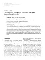
Figure 1: Receiver block diagram.
combined with Square-Root linear MMSE detection was
selected and its hardware architecture is described in
Section 5. The implementation results on Xilinx Virtex-2 and
Virtex-4 FPGAs are presented in Sections 6 and 7 concludes
the paper.

2. SYSTEM DESCRIPTION AND LINEAR MMSE
MIMO DETECTION
We consider a linear MMSE MIMO detector a part of an
entire 802.11n compliant 4
× 4MIMOOFDMtransceiver
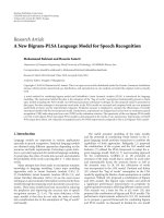
[6]. Figure 1 corresponds to the receiver block diagram.
We den ote N as the number of transmit and receive
antennas. For each subcarrier, we denote the N
× 1received
vector as y which is given in (1). Where s is the N
× 1
transmitted symbol vector, H is the N
× N channel matrix,
and n is the N
×1 additive white Gaussian noise vector with
covariance matrix N
0
·I;
y
= Hs + n. (1)
In this paper, we focus on the MIMO detector block in
Figure 1 which produces the linear MMSE solution

y, the
estimate of the transmitted symbol vector s, and the effective,
post detection, noise variance vector

n.

y and


n are given by
(2)and(3)[4, 22]:

y =

H
∗
H + N
0
·I

−1
·H
∗
y = W
MMSE
·y,
(2)

n = diag

E


y −s


y −s


∗

=
diag

N
0
·

H
∗
H + N
0
·I

−1

,
(3)
where (
·)
∗
is a conjugate-transpose operation and diag (·)
represents the mapping of the diagonal components of a
matrix to a column vector.
It is worth noting that as part of an entire MIMO
system, the MIMO detector output will feed into a soft
decision FEC (forward error correction) decoder, which in
turn needs to calculate the log likelihood ratios (LLRs). The
LLR calculations [21, 23] need the


n estimates which will be
provided by the proposed MIMO detector block. Note that

n output from the MIMO detector is required only when
the soft decision metric is used for FEC decoding. In our
system, the linear MMSE detector provides

y
k
and

n
k
to the
100
200
300
400
500
600
700
800
900
1000
1100
Slices
14 15 16 17 18 19 20 21 22
Precision
Complexity ratio = (silces for a CORDIC/slices for a multiplier)

∗
100
CORDIC
Multiplier
Multiplier versus CORDIC complexity
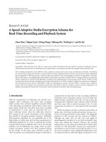
Figure 2: Hardware Complexity of a CORDIC or Multiplier.
kth soft bit decision computation block (see Figure 1), where

y =


y
1
···

y
N

T
and

n =


n
1
···

n
N


T
.
3. A COMPREHENSIVE MEASURE OF
ALGORITHMIC COMPLEXITY
Before we start to analyze the complexity of alternative
MMSE MIMO detection algorithms, it is necessary to define
a realistic and comprehensive measure of algorithm com-
plexity. The traditional technique for estimating algorithm
complexity is to simply count the number of operations.
However, the operation count alone is not a sufficient
measure to estimate realistic algorithm complexity especially
when we consider fixed point precision issues. To illustrate
this, consider Figure 2 which shows the FPGA slice count
for a CORDIC operator and a lookup table-based multiplier
synthesized on a Xilinx Virtex-2 FPGA. We have chosen these
operators since all the candidate MMSE detection algorithms
being considered here are either CORDIC or multiplier
intensive.
4 EURASIP Journal on Advances in Signal Processing
Figure 2 clearly shows that the hardware complexity of
a CORDIC operator or a multiplier is linearly proportional
to its bit precision and the slice count ratio between two
operators can be approximated as a constant within a
wide precision range (14
∼ 22 bits). We propose a more
comprehensive metric for measuring the complexity of an
algorithm. The new metric is defined in (4) and is termed
the “adjusted operation counts”. It takes into account the
bit precision of the operator, the relative complexity of the

operator, and naturally the number of operations. We will
adopt this metric throughout the paper;
Adjusted Operation Counts
=
M

m=1
α
m

b
1
m
+ b
2
m
b
0

,(4)
where M is the total number of operations, b
0
is a normal-
ization factor, b
i
m
is the bit precision of the ith input operand
of the mth operation and α
m
is the relative complexity

coefficient of the mth operation.
Normalizing our operations to 16-bit precision multipli-
cations, we let b
0
= 32 (corresponding to two 16-bit preci-
sion operands) and set α
m
= 1 when the mth operation is
a multiplication. When comparing multiplier and CORDIC
operations in FPGA implementation, we will assume that
for the same precision, the CORDIC operation has 3.5
times higher hardware complexity than the multiplication as
Figure 2 indicates (α
m
= 3.5 for a CORDIC). In this vein,
a 24-bit precision multiplication is regarded as 1.5 effective
operations (1.5 in adjusted operation counts) while a 24-bit
precision CORDIC operation is counted as 5.25 in adjusted
operation counts.
4. LINEAR MMSE DETECTION ALGORITHM
COMPARISON
All the MMSE detector implementations reported in the
literature [17–20] use a Squared MMSE formulation of the
MIMO detector problem with an explicit matrix inversion of
(H
∗
H + N
0
·I)
−1

. Of these, [17, 19, 20]useQRdecomposi-
tion to solve the matrix inversion problem.
A QR decomposition-based Squared MMSE formulation
is given in (5)–(8):
A
S
= H
∗
H + N
0
·I,
(5)
QR decomposition: A
S
= Q
S
R
S
=⇒ A
−1
S
= R
−1
S
Q
∗
S
,
(6)


y
= R
−1
S
Q
∗
S
H
∗
y = W
MMSE
·y,
(7)

n
= diag

N
0
·R
−1
S
Q
∗
S

.
(8)
The Square-Root MMSE formulation (9)–(11)[14, 22]
exploits the structure of the compound matrix


H
√
N
0
I

in order to eliminate the need for matrix inversion. It
also significantly reduces the precision requirements of the
system, as will be seen in later sections. The Square-Root
MMSE formulation was first introduced in [14]whereit
was used in the implementation of V-BLAST-type detectors
[16, 22]. Its application to the linear MMSE MIMO detector
has hitherto been unexplored and is one of the contributions
of the present work;
A
1/2
SQ
=

H

N
0
·I

=
Q
SQ
R

SQ
=

Q
1
Q
2

R
SQ
,(9)

N
0
·I = Q
2
R
SQ
, R
−1
SQ
=
Q
2

N
0
,

y =

Q
2

N
0
Q
∗
1
y = W
MMSE
·y,
(10)

n = diag

Q
2
·Q
∗
2

. (11)
One interesting fact about the Square-Root formulation
is that both R
SQ
and Q
2
are upper triangular matrices. In later
section, we will exploit this property to help us reduce the
number of hardware multipliers.

In order to come up with the best implementation, we
carried out a side by side comparison of four alternative
linear MMSE detection algorithms and chose the one with
the lowest adjusted operations count metric. These four
alternatives are
(1) Squared MMSE formulation with QR decomposition
using Givens rotations,
(2) Squared MMSE with QR decomposition using mod-
ified Gram-Schmidt orthogonalization,
(3) Square-Root MMSE with QR decomposition using
Givens rotations,
(4) Square-Root MMSE with QR decomposition using
modified Gram-Schmidt orthogonalization.
AGivensrotation[24]canbeefficiently implemented
in hardware by using a CORDIC operator. Meanwhile,
the Gram-Schmidt orthogonalization approach for QR
decomposition was motivated by the presence of dedicated
multipliers on the target FPGA, which could provide for a
better balance in the utilization of the part. An overview of
these techniques can be found in [17, 24].
4.1. Numerical stability analysis and algorithm
complexity assessment
The adjusted operation count metric requires the minimum
acceptable signal precision for each of the four alternatives
listed above. In order to achieve this, fixed point simulations
were performed operating over the IEEE 802.11n channel
model D [25]. Our simulation setup includes a complete
IEEE 802.11n reference system including all the transmitter
and receiver elements shown in Figure 1. The simulation
parameters such as the number of subcarriers, OFDM

symbol duration, guard interval, and position of pilot
subcarriers and the others are determined according to the
IEEE 802.11n draft standard [5]. The 802.11n convolutional
encoder along with soft-decision input Viterbi decoder was
applied to the simulation. Packet size was set to 1000 bytes.
The number of antennas at the transmitter and receiver
was set to 4 and 64QAM constellation with FEC coding
rate of 2/3 was used. This configuration corresponds to
Hun Seok Kim et al. 5
10
−3
10
−2
10
−1
10
0
PER
28 29 30 31 32 33 34 35 36
SNR
Floating point
Fixed point, Square-Root, Gram-Schmidt
Fixed point, Squared, Gram-Schmidt
Fixed point, Square-Root, Givens
Fixed point, Squared, Givens
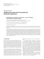
Figure 3: PER Performance of fixed point algorithms, 4 × 4
64 QAM.
MCS (Modulation and Coding Scheme) 29 in the 802.11n
specification. This particular configuration requires higher
SNR than most other modulation and coding schemes in

the 802.11n standard and as such will be more sensitive to
the quantization noise and stability issues that plague finite
precision systems.
The required bit precisions for the four alternative detec-
tor algorithms are presented in Ta ble 1. The bit precisions
were determined through a Monte-Carlo-based study that
plotted the packet error rate (PER) for the end to end system
with the aim of finding the required signal precision that
resulted in a precision loss of less than 0.5 dB. We define preci-
sion loss as the difference in SNR required to achieve 1% PER
when using floating point precision and when using fixed
point precision. The required bit precision for each interme-
diate matrix (e.g., R
−1
S
in Tab le 1 ) was obtained in isolation
assuming that all other matrices were represented with float-
ing point. After we obtained the required bit precisions for all
intermediate matrices, they were combined and fine-tuned
together via incremental precision modifications until we
achieve the target precision loss. The PER curves in Figure 3
show the fixed point design performance of our system where
all matrices and corresponding arithmetic operations are
represented with finite bit precisions specified in Tab l e 1.In
general, more bit precisions are required to operate at higher
SNRs where numerical stability issues become critical due to
the higher condition number of the matrix H
∗
H + N
0

·I.
It is worth noting that the required bit precisions
for modified Gram-Schmidt QR decomposition are higher
than those for the Givens rotation-based QR in both the
Squared and the Square-Root MMSE detection cases. The
better numerical stability of Givens rotation comes from
its unitary transformation property which preserves the
200
400
600
800
1000
1200
1400
Operations
22.533.544.55
N
Squared Gram-Schmidt
Squared Givens
Square-Root Gram-Schmidt
Square-Root Givens
Figure 4: Operation count for each algorithm.
magnitude. However, in the Square-Root MMSE formula-
tion, the difference of the required bit precision between
Gram-Schmidt and Givens rotation-based methods becomes
smaller. This is because of the structure of the Square-
Root algorithm. That is, the lower half rows of the matrix
A
1/2
SQ

in the Square-Root algorithm have very small values
at high SNR and become the main impediments for the
Givens rotation method in computing accurate rotation
angles. On the contrary, the same problem is not critical
in the Gram-Schmidt method since its Q
SQ
computation
is based on an entire column vector rather than only two
components of the column vector. Moreover, we observe
that the bit precision requirement of the modified Gram-
Schmidt QR decomposition method is significantly relaxed
in Square-Root detection since neither R
SQ
nor R
−1
SQ
is
involved in the detection process. In the following section,
we will introduce a dynamic scaling technique which will
further improve the numerical stability of modified Gram-
Schmidt QR decomposition in Square-Root MMSE detec-
tions.
In order to use the adjusted operation counts as a realistic
measure of algorithm complexity, the number of operations
for each algorithm needs to be specified. This is shown
in Tab le 2. Most of the arithmetic operations involved in
MMSE algorithms take complex numbers as input. When
counting the number of operations in Ta bl e 2,weequatea
complex multiplication to 3 real multiplications [26] while
vectoring and rotating CORDIC operations on complex

numbers are counted as 2 and 3 real CORDIC operations,
respectively [16, 17]. Figure 4 shows the operation counts
(sum of the number of multiplication, division, square-root
and CORDIC operations) for computing W
MMSE
and

n as a
function of the number of antennas N.
6 EURASIP Journal on Advances in Signal Processing
Table 1: Required bit precisions.
Fixed point computation
Squared MMSE algorithm Square-Root MMSE algorithm
Gram-Schmidt QR-based Givens QR-based Gram-Schmidt QR-based Givens QR- based
H, N
0
I (input) 14 14
A
s
or A
1/2
SQ
14 19 16
Q
S
or Q
SQ
25 15 19 16
R
S

or R
SQ
27 17 21 18
R
−1
S
20 Not required
A
−1
S
= R
−1
S
Q
∗
S
20 Not required
1

N
0
Q
2
Not required 14
W
MMSE
16 14

n = diag


N
0
·A
−1
S

=
diag

Q
2
Q
∗
2

16 14
Table 2: Operation counts for computing W
MMSE
and

n.
Real value input operations
Squared MMSE Square-Root MMSE
Gram-Schmidt QR Givens rotation QR Gram-Schmidt QR Givens rotation QR
Multiplications
21
2
N
3
+7N

2
−
1
2
N
15
2
N
3
+6N
2
−
1
2
N
11
2
N
3
+5N
2
+
5
2
N
3
2
N
3
+

7
2
N
2
Divisions NNN+1 1
Square roots N 0 N +1 1
CORDIC operations 0
5
2
N
3
+
3
2
N
2
−2N 03N
3
+7N
2
−N −1
Combining the bit precisions in Ta bl e 1 and the opera-
tion counts for each algorithm in Ta bl e 2 ,wecancompute
the adjusted operation counts for all algorithms. In adjusted
operation counts computation (4), we set α
m
= 0for
additions (the relative hardware complexity of an addition
is 0) because they take much lower resources in FPGAs than
multiplications or CORDIC operations. Furthermore, since

all algorithms require a small number (less than N +2)of
divisions and square-root operations, a single time-shared
divider and square-root operator will be sufficient for each
algorithm when N is reasonably small (i.e., less than 6).
Consequently, the hardware complexity involved in division
and square-root operations will be assumed to be the same
for all MMSE detection algorithms. Therefore, in this work,
we compute adjusted operation counts by only considering
multiplications (α
m
= 1) and CORDIC operations (α
m
=
3.5). The adjusted operation counts for a 4 × 4MIMO
detector are shown in Tabl e 3 . It is seen that the Square-
Root MMSE detection algorithms require significantly less
hardware resources than their Squared MMSE counterparts.
4.2. Algorithm enhancement:
dynamic scaling technique
It is well known that the modified Gram-Schmidt QR
decomposition has an advantage in numerical stability when
compared to the original Gram-Schmidt algorithm [24].
In addition, we have found that this algorithm when used
in a Square-Root MMSE detector can be made even more
efficient by exploiting the fact that the R
SQ
matrix, which
results from the QR decomposition, does not contribute to
the MMSE solution. Essentially, we can apply any processing
to A

1/2
SQ
as long as Q
SQ
remains unchanged, even if it does not
preserve R
SQ
.Aswecanseefrom(12), dynamic scaling of the
ith column, v
i
, with an arbitrary constant c
i
has the property
of preserving the Q
SQ
matrix but not necessarily R
SQ
:
A
1/2
SQ
=

v
1
v
2
··· v
N


=Q
SQ
·R
SQ
=

u
1
u
2
··· u
N

·R
SQ
=⇒

A
1/2
SQ
=

c
1
v
1
c
2
v
2

··· c
N
v
N

= Q
SQ
·

R
SQ
=

u
1
u
2
··· u
N

·

R
SQ
.
(12)
The modified and scaled Gram-Schmidt QR decomposi-
tion for the Square-Root MMSE solution with the recursive
dynamic scaling step is shown in Algorithm 1. The dynamic
scaling steps correspond to steps (d)–(g) in Algorithm 1.

By exploiting this recursive scaling, we can guarantee that
the maximum absolute value of the real or imaginary
components of the vector v
j
is always within a predefined
range. The significance of the dynamic scaling technique
on Gram-Schmidt QR decomposition comes from the fact
that each column orthogonalization makes the magnitude
of the projection columns (v
j
:= v
j
− r
ij
·u
i
)become
smaller as the recursive orthogonalization step continues. In
order to resolve this problem, we introduced steps (d)–(e)
in Algorithm 1. It makes the magnitude of the projection
vector v
j
always greater than a certain threshold so that we
Hun Seok Kim et al. 7
Table 3: Adjusted operation counts for computing W
MMSE
and

n (4 ×4 detector).
Squared MMSE Square-Root MMSE

Givens rotation QR-based Gram-Schmidt QR-based Givens rotation QR-based Gram-Schmidt QR-based
Adjusted operation counts 1150.50 872.50 780.84 488.44
(a) A
1/2
SQ
=

H

N
0
·I

=

v
1
v
2
··· v
N

(b) for
i
= 1toN
(c) for
j
= i to N
(d) while
(max

{|R(ν
1,j
)|, |I(ν
1,j
)|, , |I(ν
2N,j
)|} < 2
L
)
(e) v
j
:= 2v
j
(f) while (max{|R(ν
1,j
)|, |I(ν
1,j
)|, , |I(ν
2N,j
)|} > 2
U
)
(g)
v
j
:= v
j
/2
(h) end
(i) r

ii
:=v
i
, u
i
:=
v
i
v
i

(j) for
j
= i +1 toN
(k)
r
ij
:= u
∗
i
·v
j
(l) v
j
:= v
j
−r
ij
·u
i

(m) end
(n) end
Algorithm 1: The modified and scaled Gram-Schmidt QR decomposition (v
i
= [ν
1,i
··· ν
2N,i
]
T
, R(·)andI(·) stand for real and
imaginary parts of a complex number, respectively, Q
SQ
= [u
1
··· u
N
], L and U are predefined lower and upper bounds).
10
−3
10
−2
10
−1
10
0
PER
28 29 30 31 32 33 34 35 36
SNR
Floating point

With dynamic scaling, fixed point: 14-bit Q, 16-bit R
With dynamic scaling, fixed point: 12-bit Q, 14-bit R
No dynamic scaling, fixed point: 14-bit Q, 16-bit R
No dynamic scaling, fixed point: 18-bit Q, 20-bit R
No dynamic scaling, fixed point: 19-bit Q, 21-bit R
Figure 5: Impact of dynamic scaling on Gram-Schmidt QR.
can activate the full dynamic range all the time. Dynamic
scaling also prevents r
ii
(namely, v
j
) from becoming a very
large number and consequently the dynamic range of 1/
v
j

can be controlled such that it does not exceed the desired
precision. This improves the numerical stability of v
i
/v
i
,
while maintaining low bit precision.
The dynamic scaling technique is unique to Square-Root
MMSE detection. The preprocessing such as (12) cannot
be applied to Squared MMSE detection since its solution
depends on both R
S
and Q
S

of the QR decomposition
process. Hence, this type of dynamic scaling technique had
not been exploited in previous works [17–20], which were
based on the Squared MMSE formulation.
The impact of recursive dynamic scaling on a modified
Gram-Schmidt QR-based Square-Root MIMO detection
algorithm is shown in Figure 5 and Tab le 4.Onaverage,5
bits of precision is saved in the fixed point QR decomposition
which makes the modified Gram-Schmidt QR-based Square-
Root algorithm more hardware friendly. Note that a similar
technique can be applied to Givens rotation-based QR
decomposition in Square-Root MMSE detection. However,
the impact of the dynamic scaling on a Givens rotation
QR-based Square-Root algorithm is not as significant (see
Ta bl e 4) due to the already well-behaved numerical prop-
erties of that algorithm. As Tab le 4 shows, the proposed
dynamic scaling technique enhances the numerical stability
of the modified Gram-Schmidt QR decomposition to a level
that is comparable to the unitary transform-based QR.
The adjusted operation counts in Ta ble 5 show the algo-
rithm complexity both with and without dynamic scaling.
As shown there, Square-Root MMSE detections (even with-
out dynamic scaling) are approximately 40% less complex
8 EURASIP Journal on Advances in Signal Processing
Table 4: Required bit precisions of QR decomposition for Square-Root detection.
Givens rotation-based QR Gram-Schmidt-based QR
Without dynamic scaling With dynamic scaling Without dynamic scaling With dynamic scaling
A
1/2
SQ

, Q
SQ
16 14 19 14
R
SQ
18 16 21 16
Precisions for all other matrices Same as Ta bl e 1
OFDM symbol duration
with short GI
= 3.6 μs
Throughput  52 channels per 3.6 μs
= 14.4 M channels/s
3.6 μs3.6 μs
LT F ( N
−1) LTF (N)Datasymbol1···
·········
···
···
··· ···
···
FFT output:
Sub
carrier 1
SC 2 SC 52
y
1
y
2
y
52

H
1
H
2
H
52
Channel
estimation
latency
W
MMSE
computation
latency
W
1
W
2
W
52

n
1

n
2

n
52
W
y

:

y
1

y
2

y
52
Figure 6: MIMO detection interface timing.
compared to Squared MMSE detection. In addition, the
proposed dynamic scaling technique provides nearly 20%
additional saving in hardware complexity for the Gram-
Schmidt QR-based Square-Root MIMO detector.
Remark that when one considers hardware implementa-
tion on an FPGA, multiplication-intensive methods such as
the modified Gram-Schmidt QR decomposition are usually
more desirable than a CORDIC-intensive Givens rotation
QR algorithm because (a) dedicated multipliers are available
in FPGAs without extra cost, whereas CORDIC operators
would consume significant number of FPGA slices (see
Figure 2); (b) the latency of a pipelined CORDIC operator
is linearly proportional to its bit precision while a dedicated
multiplier on an FPGA has a single-clock latency. Based
on the complexity assessment in this section and the fact
that we target an FPGA implementation where a number
of dedicated multipliers are available, we select the modified
Gram-Schmidt QR decomposition combined with Square-
Root MMSE MIMO detection as the algorithm for our

hardware implementation. Dynamic scaling technique is also
applied to the hardware design in order to reduce its bit
precision requirement of the design.
5. HARDWARE IMPLEMENTATION ON FPGAs
The exploration of the algorithmic space in the prior sections
led us to an algorithmic solution with the smallest adjusted
operation count for a given performance. In this section,
we continue to optimize the design by making tradeoffs
and enhancements at the hardware architecture level. The
primary tradeoffs made at this level are (i) time-sharing of
multiplier resources; (ii) maximizing hardware utilization
by exploiting the sparsity of some matrices; and (iii) an
efficient implementation of the dynamic scaling procedure.
These three techniques are elaborated in this section where
the performance gain for each is clearly discussed. The result
is an FPGA-based implementation that not only meets the
requirements for this work, but is also quite superior to other
detectors appearing in the recent literature.
5.1. MIMO detector overview and interface
For each subcarrier, the inputs to the MIMO detector are the
N
× N channel matrix H and the N × 1receivevectory.
Figure 6 shows the interface timing diagram of the MIMO
detector for our IEEE 802.11n test case. This test case
corresponds to a 4
× 4MIMOOFDMsystemwith52data
subcarriers and an OFDM symbol duration of 3.6 μs.
The 802.11n packet structure includes several training
symbols referred to as LTFs (long training fields) for the
purpose of estimating the channel matrices for each of the

52 data subcarriers. After the last LTF symbol is processed,
channel estimate matrices are fed into the MIMO detector.
Upon the delivery of the first channel estimation matrix
(corresponding to the first subcarrier) to the MIMO decoder,
the decoder must produce the MMSE weight matrix W
MMSE
Hun Seok Kim et al. 9
Table 5: Adjusted operation counts for computing W
MMSE
and

n (4 ×4 MMSE detection).
Squared MMSE Square-Root MMSE
Givens rotation
QR-based
Gram-Schmidt
QR-based
Givens rotation QR-based Gram-Schmidt QR-based
Dynamic scaling
Without dynamic With dynamic Without dynamic With dynamic
not available
scaling scaling scaling scaling
Adjusted operation counts
1150.50 872.50 780.84 743.46 488.44 397.81
Table 6: Place and route report.
Target FPGA Slices Number of real multipliers BRAMs
xc2v6000 (speed grade-6) 9,003 out of 33792
66 24
xc4vlx160 (speed grade-12) 7,932 out of 67854
Target FPGA Supportable operating clock frequency (f

clk
) Latency (clocks) Data throughput W
MMSE
,

n and

y,
xc2v6000 (speed grade-6) 140 MHz
388 f
clk
/8 (instances per second)
xc4vlx160 (speed grade-12) 160 MHz
and the effective noise power vector

n within 4μs. This
is per our design requirements. Figure 6 shows the timing
diagram for this sequence of events. As soon as the W
MMSE
matrix and the received vector y for the first subcarrier
become available, the MMSE detection output vector

y will
be generated by the MIMO detector. The W
MMSE
,

n,and

y computation throughput of the detector must be greater

than or equal to 14.4 M instances per second which is the
rate at which the y vectors and the channel estimates are
presented to the MIMO detector. Otherwise, the detector will
incur additional latency.
5.2. Multiplier sharing architecture
In our test case, a new 4
× 4 channel estimation matrix H is
presented to the detector at the maximum rate of φ
= 14.4M
instances per second. A fully pipelined detector must provide
W
MMSE
,

n,and

y every 69.4 ns (= 1/φ) without the need for
a FIFO and unnecessary latency. Generally, the input/output
rate φ is much lower than the maximum operating clock
frequency of the hardware. We define the multiplier time
sharing order (γ)in(13):
multiplier time sharing order (γ)
=
Operating Clock Freq. in MHz
φ
.
(13)
For our FGPA implementation, the multiplier time
sharing order is 8 implying that the minimum operating
clock frequency is 115.2 (

= 8×φ) MHz and a single multiplier
processes 8 sets of inputs within a 14.4 MHz cycle. This
specific multiplier time sharing order is naturally coupled
with the size of the compound matrix A
1/2
SQ
for the Square-
Root MIMO detector.
For the 4
× 4 Square-Root MIMO detection, A
1/2
SQ
is an
8
× 4 matrix and each step in the modified Gram-Schmidt
QR decomposition takes an 8
× 1columnvectorofA
1/2
SQ
as the input. Assuming that the matrix A
1/2
SQ
is dense, the
norm square computation steps (
v
2
) and projection vector
computation steps (u
∗
·v or r

ii
·u)eachrequire8complex
multiplications. As a result, if the multiplier can run at
a clock frequency of 115.2 MHz, the same multiplier can
be shared within a single operation step (
v
2
, u
∗
·v,or
r
ii
·u) producing the output at the rate of 14.4 M instances
per second. With this multiplier sharing architecture, the
squared Euclidean norm (
v
2
) and the v vector update
(v :
= v − (u
∗
v)·u) operations require only 2 and 6 real
multipliers, respectively.
Figures 7 and 8 show the overall architecture of the fully
pipelined 4
×4 MIMO detector with the proposed multiplier
sharing architecture. The square-root and division operator
in Figure 7 are instantiated by using Xilinx Coregen blocks
[26].
5.3. Multiplier saving techniques

The modified and scaled Gram-Schmidt QR decomposition
circuit in Figure 7 does not make use of the sparsity of the
A
1/2
SQ
matrix. Since the lower half of A
1/2
SQ
is sparse (Q
2
is upper
triangular), the multipliers in the
v
2
and the v − (u
∗
v)·u
computation are not active all the time. This can be exploited
to save multipliers when the orthogonalization is performed
on the columns of A
1/2
SQ
.InFigure 9, real multipliers in the
v
1

2
computation are active (shaded rectangles) during
only 5 out of 8 clock cycles, and complex multipliers in the
u

∗
1
v
j
computation have 4 inactive slots (unshaded rectangles)
out of 8. Meanwhile, only 5 complex multiplications are
required to compute (u
∗
1
v
j
)·u
1
and the 5th component of
u
1
is a real number. Therefore, (u
∗
1
v
j
)·u
1,1
∼(u
∗
1
v
j
)·u
1,4

can
be computed using the inactive cycles of the multipliers for
u
∗
1
v
j
computation, while (u
∗
1
v
j
)·u
1,5
can use the inactive
slots in the
v
1

2
computation. This technique provides a
saving of 17% in the required multiplier resources for the QR
decomposition circuit.
We can save additional multiplier resources in the scalar-
matrix or matrix-matrix multiplication by exploiting the
fact that some elements of the upper triangular matrix Q
2
are real numbers. Among the 10 nonzero components in
10 EURASIP Journal on Advances in Signal Processing
Table 7: Resource usage comparison.

Computation Slices Multiplier BRAM Note
This work
Q
2

N
0
6487 (Virtex2) 45 15 Corresponds to complexity of (H
∗
H + N
0
·I)
−1
W
MMSE
7679(Virtex2) 58 19 Includes 1/

N
0
·Q
2
computation
[17] W
MMSE
16865(Virtex2) 44 101
[18] α
·(H
∗
H + N
0

·I)
−1
4446(Virtex2) 101 N/A α scaling will require additional multipliers and dividers.
[19](H
∗
H + N
0
·I)
−1
86% of Virtex2
(1)
N/A N/A
[20](H
∗
H + N
0
·I)
−1
9117 (Virtex4) 22 9
(1)
The exact slice count is not available since its FPGA part name is not given.
Table 8: Throughput and latency comparison.
Output Max. throughput (million instances per second) f
clk
Latency
This work
W
MMSE
,


y,

n
17.50 140 MHz
388 clks
20.00 160 MHz
[17] W
MMSE
N/A N/A 3000 clks
[18] α
·(H
∗
H + N
0
·I)
−1
6.75
(2)
108 MHz 64 clks
[19](H
∗
H + N
0
·I)
−1
6.25
(2)
100 MHz 350 clks
[20](H
∗

H + N
0
·I)
−1
0.13
(3)
115 MHz 933 clks
(2)
The throughput is not specified in the reference. However, it can be computed from its architecture.
(3)
This is a floating point design.
v
1
v
1
v
2
v
3
v
4
v
(2)
3
v
(3)
4
v
(2)
4

v
(3)
4
v
(2)
4
v
(2)
3
v
(1)
2
v
(1)
3
v
(1)
4
v
(1)
2
Scale Scale
Scale ScaleScale
ScaleScale Scale
Scale
Scale
v
2
v
2

v
2
v
2

N
0
√
D
D
D
D
D
D
D
D
D
D
DDelaychainorRAM
Dynamic scaling
Scale
v−(u
∗
v)·u
v
−(u
∗
v)·u
v
−(u

∗
v)·u
v
−(u
∗
v)·u
v
−(u
∗
v)·u
v
−(u
∗
v)·u
1
v
1

1
v
(1)
2

1
v
(2)
3

1
v

(3)
4

1

N
0
u
1
u
2
u
3
u
4
u
1
u
3
u
2
1/x
Figure 7: QR decomposition circuit.
Hun Seok Kim et al. 11
Table 9: QR decomposition engine comparison.
QR engine output Throughput (million inst/s) Gate count Gate count per throughput Note
This work
Q
1
, Q

2
,

R
SQ
17.50 (Virtex2 FPGA, 0.120 μm) 157k
(4)
8.97 k per M inst/s
R
SQ
can be obtained
by scaling each row of

R
SQ
.
[16] Q
1
, R
SQ
1.56 (0.25 μm ASIC) 54k 34.62 k per M inst/s
R
SQ
is sorted based
on column norms
(4)
Estimated gate count from Xilinx ISE9.1 report. The QR engine was mapped, placed, and routed in isolation.
Matrix-matrix
multiplication
Construct

Q
1
, Q
2
Matrix-vector
multiplication
RAM
RAM
D
D
D
u
1
u
2
u
3
u
4
Q
2
Q
∗
1
Q
2

N
0
Q

2

N
0
Q
∗
1
1/

N
0
y

y

n
diag(Q
2
Q
∗
2
)
Figure 8: MMSE solution computation.
(u
∗
1
v
4
) ·u
1

(u
∗
1
v
3
) ·u
1
(u
∗
1
v
2
) ·u
1
u
∗
1
v
4
u
∗
1
v
3
u
∗
1
v
2
u

1
:= v
1
/v
1

2 real multipliers
3 complex multipliers
= 9 real multipliers
3 complex multipliers
= 9 real multipliers
we can save these multipliers
1/
v
1
: division

v
1

2
:sqrt
v
1

2
real multipliers
Time
Active input to operator
Idle input to operator

Figure 9: Vector orthogonalization schedule (ν
1
).
Q
2
, 4 diagonal components are real and the remaining 6
are complex. Hence, when we compute diag (Q
2
Q
∗
2
), 2 real
multipliers are sufficient with γ
= 8 time sharing. Similarly,
1/

N
0
·Q
2
(scalar-matrix) multiplication and 1/

N
0
Q
2
·Q
∗
1
(matrix-matrix) multiplication can be implemented with

2 and 13 real multipliers, respectively. It is worth noting
that on average, our design with multiplier sharing/saving
achieves 93% multiplier utilization (active time over total
time), which is 30% higher than the hardware utilization
reported in [19].
5.4. Implementation of dynamic scaling
As shown in Figure 7, the QR decomposition procedure
requires 10 identical dynamic scaling units. Thus, it is impor-
tant to implement this function in a hardware optimized
fashion. The input of the dynamic scaling circuit is an
8
× 1vectorv which corresponds to a column vector of
the compound matrix A
1/2
SQ
. We implemented a pipelined
dynamic scaling circuit where each component of the
column vector v is fed sequentially as input. Figure 10 depicts
the overall structure of the dynamic scaling circuit. The
scaling is performed in two steps. First, absolute values of the
real and imaginary parts of the input vector (all 8 elements
of the vector) are bitwise ORedandstoredinaregister
called accumulated
OR. By looking at the most significant
nonzero bit position of the accumulated
OR register, one
can verify whether the largest absolute value of v is within
the predefined range (14). Second, if the most significant
nonzero bit position of the accumulated
OR register is out

of bound, the input signals are shifted based on the position
of the most significant nonzero bit of the accumulated
OR
register. A brute-force approach for performing this most
significant nonzero bit search and barrel shift is given in the
pseudocode of Algorithm 2 where the bit precision for v is
14, the lower bound L is 11, and the upper bound is inactive
(i.e., U
= 14);
2
L
≤ max



real

ν
1



, ,


real

ν
2N




,


imag

ν
1



, ,


imag

ν
2N




≤
2
U
.
(14)
The deeply nested if-else statements shown in
Algorithm 2 combined with the barrel shift operation are

highly resource demanding when synthesized to an FPGA.
12 EURASIP Journal on Advances in Signal Processing
v real[13 : 0]
v
imag[13 : 0]
“00
···0”
prev
acced OR
[13 : 0]
abs
v re
[13 : 0]
abs
v im
[13 : 0]
ABS()
ABS()
OR Logic
next
acced OR
[13 : 0]
accumulated
OR
[13 : 0]
Find
the nonzero
MSB
+
barrel shift

scaled
v re[13 : 0]
scaled
v re[13 : 0]
···
Figure 10: Dynamic scaling circuit.
prev acced OR[13]
abc
v re[13]
abc
v im[13]
prev
acced OR[12]
abc
v re[12]
abc
v im[12]
next
acced OR[13]
next
acced OR[12]
prev
acced OR[13]
abc
v re[13]
abc
v im[13]
prev
acced OR[12]
abc

v re[12]
abc
v im[12]
prev
acced OR[11]
abc
v re[11]
abc
v im[11]
next
acced OR[13]
next
acced OR[12]
next
acced OR[11]
.
.
.
.
.
.
(a) OR Logic for brute-force search (b) OR Logic for binary search
Figure 11: OR Logic modification.
if (accumulated OR (13 : 11) > 0) then
0 bit shift;
elsif (accumulated
OR (10) = “1”) then
1 bit shift;

elsif (accumulated
OR(5) = “1”) then
6 bit shift;
else
7 bit shift;
end if;
Algorithm 2: Brute-force search and barrel shift.
The deeply nested if-else statements can be avoided by using
a binary search procedure. For the binary search, the OR logic
in Figure 10 needs to be slightly modified from the simple
bitwise OR shown in Figure 11(a) to the modified OR logic
shown in Figure 11(b). The modified OR logic performs a
nonzero-bit propagating, bitwise OR operation: once the first
nonzero most significant bit is found, the remaining less sig-
nificant bits from that position all become “1” regardless of
other inputs. The modified OR logic allows us to use binary
search, which is shown in the pseudocode of Algorithm 3.
The synthesis result for a binary search-based dynamic
scaling circuit on a Virtex2 FPGA reveals that it consumes
145 slices, whereas the brute-force approach requires 241
slices. Hence, we achieve a saving of almost 1000 slices for
the 10 dynamic scaling units needed throughout the entire
QR decomposition process. It is worth noting that without
dynamic scaling, each multiplier in the QR decomposition
would have required larger bit precision which would have
resulted in even more multiplier resources (refer to Ta bl e 1).
Given that on an FPGA (such as the Xilinx Virtex-2 or Virtex-
4family)only18
× 18 bit multipliers are available, each
multiplication with more than 18-bit precision will require

Hun Seok Kim et al. 13
if (accumulated OR(8) = “1”) then
if (accumulated
OR(10) = “1”) then
if (accumulated
OR(11) = “1”) then 0-bit shift;
else 1-bit shift;
end if;
else
if (accumulated
OR(9) = “1”) then 2-bit shift;
else 3-bit shift;
end if;
end if;
else
if (accumulated
OR(6) = “1”) then
if (accumulated
OR(7) = “1”) then 4-bit shift;
else 5-bit shift;
end if;
else
if (accumulated
OR(5) = “1”) then 6-bit shift;
else 7-bit shift;
end if;
end if;
end if;
Algorithm 3: Binary search and barrel shift.
2 dedicated multipliers. In other words, the number of

hardware multipliers required for the Gram-Schmidt-based
QR decomposition would have doubled if the proposed
dynamic scaling technique was not applied. Hence, we can
see that the dynamic scaling results in saving of 40 dedicated
multipliers in the FPGA at the cost of 1450 additional logic
slices.
6. FPGA IMPLEMENTATION RESULTS
The 4
× 4 MMSE MIMO detector design was successfully
synthesized, placed, routed, and verified on both a Xilinx
Virtex-2 and a Virtex-4 series part. These chips have a
number of dedicated hardware multipliers and two-port
block RAMs. Ta ble 6 shows the implementation result of the
IEEE 802.11n compatible MIMO detector including resource
utilization from the place and route report.
The latency of the implemented detector is 2.77 μs when
the operating clock frequency (f
clk
) is 140 MHz, which is
shorter than a single OFDM symbol in the IEEE 802.11n
draft proposal [5]. The computation throughput for W
MMSE
,

n,and

y is f
clk
/8 instances per second, which implies that
our target throughput of 14.4 M instances per second can

be met by using any f
clk
higher than 115.2 MHz. Assuming a
140 MHz clock, the implemented detector is able to compute
52 (the number of data subcarriers) W
MMSE
matrices within
2.77 μs and provide a data throughput of 420 Mbps for a
64QAM 4
×4MIMOsystem.
Ta bl es 7 and 8 show the resource usage, throughput, and
latency results for this work and some prior work in the
area. It is worth noting that none of [17–20] in Tables 7 and
8 is designed to produce a complete MMSE solution con-
sisting of both

y and

n needed for soft-decision decoding.
Additionally, [18–20] only compute (H
∗
H + N
0
·I)
−1
rather
than W
MMSE
= (H
∗

H + N
0
·I)
−1
·H
∗
= 1/

N
0
·Q
2
Q
∗
1
.For
comparison purposes, we specified the resource usage of
our design for computing 1/

N
0
·Q
2
, which corresponds to
(H
∗
H + N
0
·I)
−1

in Squared MMSE detection (compare (2)
and (10)). Ta bl e 7 shows that our design utilizes 50% and
29% fewer slices than [17, 20], respectively, while the number
of multipliers used in our design is only 45% of those in [18].
Meanwhile, the throughput of our design is at least 3 times
higher than [18–20] as shown in Ta bl e 8. The throughput of
[17] is not given but its latency is too high to meet the latency
requirements of a commercial system such as 802.11n.
Finally, we compare our QR decomposition engine (on
a Xilinx Virtex2) with an ASIC design in [16]which
implements complex CORDIC-based QR decomposition on
a0.25μm technology. The QR engine in [16] is designed for a
Square-Root MMSE V-BLAST-type detector and is similar to
the CORDIC-based QR decomposition for the Square-Root
MMSE algorithm discussed in this work. However, it is worth
noting that [16]doesnotcomputeQ
2
while it computes R
SQ
explicitly as only R
SQ
is required in a successive canceling-
based MIMO detector. Ta bl e 9 shows the throughput and
(estimated) gate counts for QR decomposition engines
in this work and the ASIC design reported in [16]. For
comparison purposes, we assume that for a given design, an
FPGA fabricated in 0.12 μm technology (Virtex2) provides
comparable speed (throughput) as an ASIC implemented in
0.25 μm. By using gate count per throughput in Tab le 9 as
the comparison metric, we observe that our design achieves

significant gain over [16].
In summary, four main techniques which together form
the major contribution of this work are responsible for this
performance gain. They are (a) definition and adoption of a
unified metric for simultaneous comparison of algorithmic
complexity and numerical stability; (b) the combination
of a modified Gram-Schmidt QR decomposition algorithm
with Square-Root linear MMSE detection resulting in a
matrix inversion free implementation; (c) a dynamic scaling
algorithm that enhances numerical stability; and (d) an
aggressive time-shared VLSI architecture. The above tech-
niques are quite general and are readily applicable to any
MMSE-based MIMO detector implementation.
7. CONCLUSION
In this paper, we studied hardware friendly algorithms that
avoid matrix inversion for linear MMSE MIMO detection.
We assessed algorithm complexity in terms of number of
operations and bit precisions in fixed point designs, while
considering FPGA implementation where a fixed number of
dedicated hardware multipliers are available. We suggested
a dynamic scaling technique for modified Gram-Schmidt
QR decomposition that increases the numerical stability of
the fixed point design. The resulting MIMO detector was
successfully implemented and demonstrated on an FPGA.
The designed 4
× 4 linear MMSE MIMO detector is capable
of complying with the proposed IEEE 802.11n standard.
14 EURASIP Journal on Advances in Signal Processing
REFERENCES
[1] G. J. Foschini and M. J. Gans, “On limits of wireless com-

munications in a fading environment when using multiple
antennas,” Wireless Personal Communications,vol.6,no.3,pp.
311–335, 1998.
[2] I. Telatar, “Capacity of multi-antenna Gaussian channels,”
European Transactions on Telecommunications, vol. 10, no. 6,
pp. 585–595, 1999.
[3] A. J. Paulraj and C. B. Papadias, “Space-time processing for
wireless communications,” IEEE Signal Processing Magazine,
vol. 14, no. 6, pp. 49–83, 1997.
[4] A. J. Paulraj, D. A. Gore, R. U. Nabar, and H. B
¨
olcskei,
“An overview of MIMO communications—a key to gigabit
wireless,” Proceedings of the IEEE, vol. 92, no. 2, pp. 198–217,
2004.
[5] IEEE TGn Working Group, “Joint Proposal: High through-
put extension to the 802.11 Standard,” e802.
org/11/.
[6] J. Chen, W. Zhu, B. Daneshrad, et al., “A real time 4
× 4
MIMO-OFDM SDR for wireless networking research,” in
Proceedings of the 15th European Signal Processing Conference
(EUSIPCO ’07),Pozna
´
n, Poland, September 2007.
[7] C. M. Rader, “MUSE-a systolic array for adaptive nulling
with 64 degrees of freedom, using Givens transformations
and wafer scale integration,” in Proceedings of the International
Conference on Application Specific Array Processors, pp. 277–
291, Berkeley, Calif, USA, August 1992.

[8] K. Raghunath and K. Parhi, “A 100 MHz pipelined RLS
adaptive filter,” in Proceedings of IEEE International Conference
on Acoustics, Speech, and Signal Processing (ICASSP ’95), vol. 5,
pp. 3187–3190, Detroit, Mich, USA, May 1995.
[9] A. Burg, N. Felber, and W. Fichtner, “A 50 Mbps 4
× 4
maximum likelihood decoder for multiple-input multiple-
output systems with QPSK modulation,” in Proceedings of
the 10th IEEE International Conference on Electronics, Circuits
and Systems (ICECS ’03), vol. 1, pp. 332–335, Sharjah, UAE,
December 2003.
[10] A. Burg, M. Borgmann, M. Wenk, M. Zellweger, W. Fichtner,
and H. B
¨
olcskei, “VLSI implementation of MIMO detection
using the sphere decoding algorithm,” IEEE Journal of Solid-
State Circuits, vol. 40, no. 7, pp. 1566–1576, 2005.
[11] Z. Guo and P. Nilsson, “A VLSI architecture of the Schnorr-
Euchner decoder for MIMO systems,” in Proceedings of
the 6th IEEE Circuits and Systems Symposium on Emerging
Technologies: Frontiers of Mobile and Wireless Communication,
vol. 1, pp. 65–68, Shanghai, China, May-June 2004.
[12] K W. Wong, C Y. Tsui, R. S K. Cheng, and W H. Mow,
“A VLSI architecture of a K-best lattice decoding algorithm
for MIMO channels,” in Proceedings of IEEE International
Symposium on Circuits and Systems (ISCAS ’02), vol. 3, pp.
273–276, Phoenix, Ariz, USA, May 2002.
[13] P. W. Wolniansky, G. J. Foschini, G. D. Golden, and R.
A. Valenzuela, “V-BLAST: an architecture for realizing very
high data rates over the rich-scattering wireless channel,” in

Proceedings of the URSI International Symposium on Signals,
Systems, and Electronics (ISSSE ’98), pp. 295–300, Pisa, Italy,
September-October 1998.
[14] B. Hassibi, “An efficient square-root algorithm for BLAST,”
in Proceedings of IEEE International Conference on Acoustics,
Speech and Signal Processing (ICASSP ’00), vol. 2, pp. 737–740,
Istanbul, Turkey, June 2000.
[15] Z. Guo and P. Nilsson, “A low-complexity VLSI architecture
for square root MIMO detection,” in Proceedings of the
IASTED International Conference on Circuits, Signals, and
Systems (CSS ’03), pp. 304–309, Cancun, Mexico, May 2003.
[16] P. Luethi, A. Burg, S. Haene, D. Perels, N. Felber, and W.
Fichtner, “VLSI implementation of a high-speed iterative
sorted MMSE QR decomposition,” in Proceedings of IEEE
International Symposium on Circuits and Systems (ISCAS ’07),
pp. 1421–1424, New Orleans, La, USA, May 2007.
[17] M. Myllyl
¨
a,J M.Hintikka,J.R.Cavallaro,M.Juntti,M.
Limingoja, and A. Byman, “Complexity analysis of MMSE
detector architectures for MIMO OFDM systems,” in Proceed-
ings of the 39th Asilomar Conference on Signals, Systems and
Computers, pp. 75–81, Pacific Grove, Calif, USA, October-
November 2005.
[18] I. LaRoche and S. Roy, “An efficient regular matrix inversion
circuit architecture for MIMO processing,” in Proceedings
of IEEE International Symposium on Circuits and Systems
(ISCAS ’06), pp. 4819–4822, Island of Kos, Greece, May 2006.
[19] F. Edman and V.
¨

Owall, “A scalable pipelined complex
valued matrix inversion architecture,” in Proceedings of IEEE
International Symposium on Circuits and Systems (ISCAS ’05),
vol. 5, pp. 4489–4492, Kobe, Japan, May 2005.
[20] M. Karkooti, J. R. Cavallaro, and C. Dick, “FPGA imple-
mentation of matrix inversion using QRD-RLS algorithm,” in
Proceedings of the 39th Asilomar Conference on Signals, Systems
and Computers, pp. 1625–1629, Pacific Grove, Calif, USA,
October-November 2005.
[21] I. B. Collings, M. R. G. Butler, and M. R. McKay, “Low
complexity receiver design for MIMO bit-interleaved coded
modulation,” in Proceedings of the 8th IEEE International
Symposium on Spread Spectrum Techniques and Applications
(ISSSTA ’04), pp. 12–16, Sydney, Australia, August-September
2004.
[22] R. B
¨
ohnke, D. W
¨
ubben, V. K
¨
uhn, and K D. Kammeyer,
“Reduced complexity MMSE detection for BLAST archi-
tectures,” in Proceedings of IEEE Global Telecommunications
Conference (GLOBECOM ’03), vol. 4, pp. 2258–2262, San
Francisco, Calif, USA, December 2003.
[23] F. Tosato and P. Bisaglia, “Simplified soft-output demapper
for binary interleaved COFDM with application to HIPER-
LAN/2,” in Proceedings of IEEE International Conference on
Communications (ICC ’02), vol. 2, pp. 664–668, New York, NY,

USA, April-May 2002.
[24] G. H. Golub and C. F. Van Loan, Matrix Computations, Johns
Hopkins University Press, Baltimore, Md, USA, 3rd edition,
1996.
[25] IEEE TGn Working Group, “TGn Channel Models,” http://
www.ieee802.org/11/.
[26] />