Báo cáo hóa học: " Research Article Fair Adaptive Bandwidth and Subchannel Allocation in the WiMAX Uplink" pptx

Hindawi Publishing Corporation
EURASIP Journal on Wireless Communications and Networking
Volume 2009, Article ID 918261, 13 pages
doi:10.1155/2009/918261
Research Article
Fair Adaptive Bandwidth and Subchannel
Allocation in the WiMAX Uplink
Antoni Morell, Gonzalo Seco-Granados, and Jos
´
eL
´
opez Vicario
Telecommunications and System Engineering Department (TES), Autonomous University of Barcelona (UAB), 08193 Bellaterra, Spain
Correspondence should be addressed to Antoni Morell,
Received 2 July 2008; Revised 22 November 2008; Accepted 29 December 2008
Recommended by Ekram Hossain
In some modern communication systems, as it is the case of WiMAX, it has been decided to implement Demand Assignment
Multiple Access (DAMA) solutions. End-users request transmission opportunities before accessing the system, which provides an
efficient way to share system resources. In this paper, we briefly review the PHY and MAC layers of an OFDMA-based WiMAX
system, and we propose to use a Network Utility Maximization (NUM) framework to formulate the DAMA strategy foreseen in
the uplink of IEEE 802.16. Utility functions are chosen to achieve fair solutions attaining different degrees of fairness and to further
support the QoS requirements of the services in the system. Moreover, since the standard allocates resources in a terminal basis
but each terminal may support several services, we develop a new decomposition technique, the coupled-decompositions method,
that obtains the optimal service flow allocation with a small number of iterations (the improvement is significant when compared
to other known solutions). Furthermore, since the PHY layer in mobile WiMAX has the means to adapt the transport capacities
of the links between the Base Station (BS) and the Subscriber Stations (SSs), the proposed PHY-MAC cross-layer design uses this
extra degree of freedom in order to enhance the network utility.
Copyright © 2009 Antoni Morell et al. This is an open access article distributed under the Creative Commons Attribution License,
which permits unrestricted use, distribution, and reproduction in any medium, provided the original work is properly cited.
1. Introduction
The wireless community has recently directed much atten-

tion on a variety of topics related to Worldwide Interop-
erability for Microwave Access (WiMAX) technologies as
a broadband solution. Two different standards are under
this commercial nomenclature: the IEEE 802.16 [1], with its
extension to mobile scenarios IEEE 802.16e [2], and the ETSI
HiperMAN [3]. Operating in the range of 2 GHz to 11 GHz,
WiMAX enables a fast deployment of the network even in
remote locations with low coverage of wired technologies,
such as the Digital Subscriber Loop (DSL) family, and it can
be used, among others, for wireless backhaul or last-mile
applications.
The IEEE 802.16 standards family provides manufactur-
ers with basically four different physical (PHY) layers [4].
Two of them are based on single carrier transmissions and
use Time Division Multiple Access (TDMA) whereas the
other two are based on multicarrier modulations and use
either TDMA or Orthogonal Frequency Division Multiple
Access (OFDMA). Within the multicarrier subgroup, the
WirelessMAN Orthogonal Frequency Division Multiplexing
(OFDM) uses a 256-point Fast Fourier Transform- (FFT-)
based OFDM modulation together with a TDMA scheme
to deploy a Point-to-Multipoint (PMP) subnetwork in the
frequency range from 2 GHz up to 11 GHz in Non-Line-of-
Sight (NLOS) propagation conditions. This PHY layer has
been accepted for fixed WiMAX applications, and it is often
termed as fixed WiMAX. Finally, WirelessMAN OFDMA
exploits the multicarrier principles to implement a more
flexible OFDMA access scheme. As in WirelessMAN OFDM,
it is intended for NLOS PMP applications in the 2 GHz–
11 GHz range. However, it uses a variable-size FFT ranging

from 128 up to 2048 subcarriers. This PHY layer has been
accepted for mobile WiMAX applications, and it is usually
termed mobile WiMAX.
Concerning network topology, the basic configuration
is PMP with a Base Station (BS) serving many Subscriber
Stations (SSs). Not with standing, there is also a mesh
mode available where SSs can be linked directly to the
BS or routed through other SSs. This last mode is out
of the scope of this paper, where we consider the design
2 EURASIP Journal on Wireless Communications and Networking
of appropriate scheduling mechanisms in uplink using the
WirelessMAN OFDMA PHY layer and a PMP network. The
conceived scheduling mechanism is based on a Demand
Assignment Multiple Access (DAMA) strategy that imple-
ments a Dynamic Bandwidth Allocation (DBA) solution
(where bandwidth is understood as rate in a wide sense).
Jointly with flow allocation, we consider the adjustment
of the transmission parameters of the OFDM system, and
hence, the joint approach proposes a cross-layer interaction
between PHY and Medium Access Control (MAC) system
layers.
Previous works related to Radio Resource Management
(RRM) in WiMAX networks address a variety of scenarios,
from PMP to mesh, from TDMA to OFDMA access types,
and distinguishing single channel or multichannel networks,
most of them from a physical (PHY) layer perspective,
where the goal is to properly configure the transmission
parameters. At the best of our knowledge, two main
approaches are found in literature, namely: (i) formulate
the problem in a mathematical optimization framework and

(ii) develop heuristic algorithms. In the sequel, we briefly
review some of the works. In [5], the author proposes
an heuristic solution for the case of a single cell OFDMA
WiMAX network that maximizes the network sum-rate
under some fairness considerations by means of performing
subcarrier and power allocation. The authors in [6]analyze
how concurrent transmissions boost performance in mesh
type networks by proposing an interference-aware routing
and scheduling mechanism. In [7], the reader can find a
discussion about the advantages of a multichannel network.
Finally, [8] contributes with a mathematical optimization
solution that falls into the Network Utility Maximization
(NUM) framework, where a distributed optimal solution to
the established NUM problem is obtained using a convex
decomposition approach. The authors extend in [9] their
original work to generic OFDMA mesh networks, and the
contributions in [10–12] are within the same context. A
common feature in the last three references is that they split
the global rate control and resource allocation problem into
independent and smaller subproblems in order to alleviate
the complexity of the solution at the expenses of a certain
loss in optimality.
Our work follows the NUM framework to define the
underlying optimization problem as in [8] but modifies the
formulation in order to exactly fit the DAMA process that
is envisaged for the WiMAX uplink. The problem is then
decomposed (without any loss in optimality) using the Mean
Value Cross (MVC) decomposition method [13]. It allows to
separate the original joint problem into a flow optimization
problem (given fixed link capacities) and a radio resource

optimization problem (given fixed values of transmission
rates). The latter results in a linear program that can be
solved centrally at the BS, whereas a distributed solution that
uses the novel proposed coupled-decompositions method is
applied to the former.
The rest of the paper is organized as follows. Section 2
describes the system model. Section 3 reviews the MVC
decomposition technique and introduces the novel coupled-
decompositions method, whereas Section 4 solves the pro-
posed joint problem in Section 2. Finally, Section 5 gives
some numerical results, and Section 6 ends the paper with
the conclusions.
2. System Model
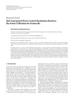
Let us consider a PMP OFDMA WiMAX network as depicted
in Figure 1, where a number of SSs share a subset of the
subchannels in the system. A subchannel in WiMAX is
made up of some of the system subcarriers and lasts for
several OFDM symbols in time. There exist different ways
to gather subcarriers into subchannels, which depend on the
permutation types (see in [4] a good review on WiMAX
aspects). In this work, we assume that the transmitting power
per subchannel as well as the set of subcarriers that form it
is given. Therefore, the different powers are not variables of
our allocation problem. Furthermore, each terminal allocates
the amount of power at each subchannel among the inner
subcarriers in order to optimize the transmitting rate. This
assumption can be found in [14], where the authors take into
account intercell interference to constrain the subchannel
transmitting powers. Note that one interesting extension is
then the inclusion of subchannel power allocation but it is

beyond the scope of this paper. In our framework, given a
specific allocation of subchannels to terminals
{ρ
i
} (top left
part of the figure), each terminal is able to transmit at a
rate c
i
(ρ
i
), which is the sum of the rates that the SS attains
in its active subchannel subset (the subset allocated to the
terminal).
We further assume (as described in the IEEE 802.16 stan-
dard documents) that each terminal negotiates the resource
allocation for all traffic flows that go through it, that is, it
jointly requests transmission opportunities for the ongoing
connections without doing it on a flow basis. The advantage
of this procedure is that signaling is reduced, specially when a
significant number of connections have to be managed. The
disadvantage is that, depending on the particular mechanism
used to find the solution of the problem, it may not be
optimal. In that sense, solutions derived from distributed
optimization do not sacrifice optimality. The price to pay is
the time required to get the solution, and therefore, we are
interested in techniques that converge fast. In Figure 1, the
rate of the jth flow at the ith SS is labeled as r
i
j
.

The IEEE 802.16 standard defines five different schedul-
ing services that will provide Quality of Service (QoS) differ-
entiation among the multiple traffic types. These services are
[4] (i) the Unsolicited Grant Service (UGS) (ii) the real-time
Polling Service (rtPS) (iii) the non-real-time Polling Service
(nrtPS) (iv) the Best-Effort (BE) service, and (v) the extended
real-time Polling Service (ertPS). Let us model the DAMA
solution implemented in the WiMAX uplink by means of a
convex program [15] where the different scheduling services
are mapped using three parameters: the minimum rate that
has to be allocated to the connection (the jth flow at the ith
terminal) or m
i
j
, the rate requested or d
j
i
, and the priority
of the service or p
i
j
. The desired QoS degree of each service
depends then on both m
i
j
and p
i
j
. For example, the UGS
that needs a constant rate can be requested just by plugging

EURASIP Journal on Wireless Communications and Networking 3
Terminals
Subchannels
ρ
1
ρ
3
ρ
5
c
1
(ρ
1
)
c
3
(ρ
3
)
c
5
(ρ
5
)
C
BS
SS1 SS2 SS3 SS4 SS5
r
1
1

···
r
1
i
···
r
1
N
1
r
3
1
···
r
3
j
···
r
3
N
3
r
5
1
···
r
5
k
···
r

5
N
5
Figure 1: Reference model.
that rate into m
i
j
and fixing d
i
j
= m
i
j
regardless the value of
p
i
j
. Another example is the ertPS that can be requested with
some amount of m
i
j
for the fixed allocation part and some
d
i
j
>m
i
j
for the variable rate part. The value p
i

j
is then used
to prioritize this flow against other competing connections.
In summary, the cross-layer system model used to char-
acterize the DBA part of WiMAX, including PHY and MAC
layer issues, responds to the following convex optimization
problem in maximization form [15, Section 4.1.3]:
max
{r
i
j
},Γ
N

i=1
N
i

j=1
U
i
j

r
i
j
; p
i
j


s.t.
N

i=1
N
i

j=1
r
i
j
≤ C,
N
i

j=1
r
i
j
≤ c
i

ρ
i

, i = 1, , N,
m
i
j
≤ r

i
j
≤ d
i
j
, ∀i, ∀j,
Γ1  1,
ρ
i
 0, i = 1, , N,
(1)
where U
i
j
(r
i
j
; p
i
j
) is the function that measures the utility
perceived by the connection when the rate r
i
j
is allocated.
The function has p
i
j
as a parameter. Furthermore, Γ =
[ρ

1
, , ρ
N
] collects the subchannel allocation per user (ρ
i
),
and the symbols  and  stand for component-wise non-
strict inequalities. Finally, c
i
(ρ
i
) = ρ
T
i
c
i
,wherec
i
contains
the achievable rates of SS
i
at each possible subchannel, and
C is the rate at which the BS can transmit. Note that in
principle the allocation variables within each vector ρ
i
should
take the integer values 0 and 1 so that a given subchannel is
completely allocated to a certain SS, whereas the constraint
Γ1  1 forces that no more than one terminal gets the
subchannel. As it has been done in other works in literature

[16], we relax the integer constraints to ρ
k
i
≥ 0, which
allows us to represent the problem as a convex one (easy to
solve). Once the solution of the relaxed problem is found,
a suboptimal solution to the original problem (with integer
constraints) is obtained by means of employing rounding
algorithms. However, in the WiMAX scenario and taking
into account that an allocation is kept during several time-
slots, real-valued allocation variables have sense in practice
(by time sharing of subchannels). Indeed, if we consider that
the allocation lasts for T time slots, then it is possible to use
values in Γ with a granularity of 1/T.
Not with standing, the problem in (1) itself does not
guarantee a fair allocation of resources. Fortunately, such
distribution can be attained by means of employing adequate
utility functions, and a general formulation for fairness
was introduced in [17] under the nomenclature of (p,α)-
proportional fairness. A feasible rate vector r
†
(i.e., it attains
the generic network constraints Ar
†
 c)issaidtobe(p, α)-
proportionally fair (where p
= [p
1
, , p
N


]
T
and α are
positive real numbers) if, given any other feasible rate vector
r
‡
, it holds that
N


i=1
p
i
r
‡
i
−r
†
i

r
†
i

α
≤ 0, ∀r
‡
s.t. r
‡

i
≥ 0, Ar
‡
 c. (2)
Accordingly, the utility functions that accomplish this fair-
ness criterion are [17]
U
i

r
i
; p
i
, α

=
⎧
⎪
⎪
⎨
⎪
⎪
⎩
p
i
log

r
i


, α = 1,
p
i
r
(1−α)
i
1 −α
, α
/
=1.
(3)
The reader can find in Figure 2 the plots of U
i
(r
i
; p
i
, α)for
α
= 0.1, α = 1, and α = 3(equalp
i
value).
Let us fix p
= [1, ,1]
T
and move from α →∞to
α
= 0. With α →∞, the solution is said to be max-min fair
[18, Section 6.5], and it is not possible (given feasibility, i.e.,
Ar  c) to increase any rate in the network, say r

j
, without
decreasing another rate r
p
<r
j
. On the other hand, when
α
→ 0, the flow allocation problem leads to a max sum-
rate approach, and therefore, it drastically favors the users
4 EURASIP Journal on Wireless Communications and Networking
Utility versus rate (different degrees of fairness)
Utility
−8
−6
−4
−2
0
Rate
0.20.30.40.50.60.70.80.9
α
= 0.1
α
= 1
α
= 3
Figure 2: Different degrees of fairness (α) in the definition of utility
functions.
with better links (it is then unfair). Intermediate solutions
allow a certain decrease in r

p
at the expenses of a greater
increase in r
j
depending on α. Note that in Figure 2 the
bigger the α value is, the higher the increase in r
j
will be in
order to compensate a utility loss in r
p
. A common adopted
solution in literature is α
= 1, and it was termed by Kelly
[19] as proportional fair. Moreover, this solution coincides
with the Nash Bargaining one, and therefore, it accomplishes
the recognized, axioms in game theory [20] of linearity,
irrelevant alternatives and symmetry [21].
We can conclude that there is no unique criterion to
define fairness but a series of them are explicitly character-
ized with the utility functions in (3). Furthermore, some
flows can be prioritized over the others within a specific fair-
ness framework (fixed by α) by particular adjustment of the
scale thanks to the parameters
{p
i
}. In general, proportional
fairness (α
= 1) provides a reasonable trade-off between
fairness and resource utilization (network throughput).
3. Decomposition in Convex Programming

Decomposition techniques are used to break down a given
optimization problem into a number of smaller problems,
usually termed the subproblems. The most used decompo-
sition methods in communications literature and in relation
to convex optimization are primal and dual decompositions
[22, 23]. It is usual to employ these decomposition tech-
niques as a tool to obtain distributed solutions to some
problems, as it is the case in Network Utility Maximization
(NUM) problems [24, 25]. The formulation in (1)isan
adaptation of the classical NUM to match the DBA problem
in OFDMA WiMAX. Recently, Palomar and Chiang provided
an exhaustive review on primal and dual decompositions
applied to the classical NUM and extensions of it [26]. In par-
ticular, they proposed multilevel decomposition approaches
to split the problem into different and coupled subsets of
variables (e.g., link powers and transmission rates). However,
the problem in primal and dual decompositions is that, in
general, they converge slowly and that an adaptation step
size has to be fixed by the user. So motivated, we base our
work in two distinct decomposition techniques: the Mean
Value Cross (MVC) decomposition [13] and the proposed
novel coupled-decompositions method. In the following, we
briefly review the former and describe the latter.
3.1. Mean Value Cross Decomposition. Consider the follow-
ing problem formulation from [13]:
min
x,y
c(x)+e(y)
s.t. A
1

(x)+B
1
(y) ≤ b
1
,
A
2
(x)+B
2
(y) ≤ b
2
,
x
∈ X,
y
∈ Y,
(4)
where c :
R
n
1
→ R, e : R
n
2
→ R, A
1
: R
n
1
→ R

m
1
,
B
1
: R
n
2
→ R
m
1
, A
2
: R
n
1
→ R
m
2
,andB
2
: R
n
2
→ R
m
2
are convex functions. The sets X and Y are also convex and
compact. It is further assumed that strong duality holds.
Construct now the partial Lagrangian function of the

problem (4)as
L(x, y, μ)
= c(x)+e(y)+μ
T

A
1
(x)+B
1
(y) −b
1

(5)
and minimize it over the variable x, including the constraints
that have not been taken into account in the Lagrangian
definition, to obtain the function K(y, μ) as follows:
K(y, μ)
=min
x
L(x, y, μ)
s.t. A
2
(x) ≤ b
2
−B
2
(y),
x
∈ X,
(6)

which is convex in y and concave in μ [13].
From K(y, μ), the method defines the primal and the dual
subproblem by fixing either the primal variable y or the dual
variable μ. After some manipulations, the primal subproblem
turns into
p(y)
=min
x
c(x)+e(y)
s.t. A
1
(x) ≤ b
1
−B
1
(y),
A
2
(x) ≤ b
2
−B
2
(y),
x
∈ X
(7)
and the dual subproblem into
d(μ)
= min
x,y

c(x)+e(y)+μ
T

A
1
(x)+B
1
(y) −b
1

s.t. A
2
(x)+B
2
(y) ≤ b
2
,
x
∈ X,
y
∈ Y.
(8)
EURASIP Journal on Wireless Communications and Networking 5
Finally, the method is completed by passing filtered
versions of the primal and dual variables between the primal
and dual subproblems, as it is summarized in the following
algorithm.
Take starting points μ
0
 0 and y

0
∈ Y and let k = 1.
Repeat
(1) Let
μ
k
= (1/k)

k−1
i
=0
μ
k−1
= (1/k)μ
k−1
+((k −
1)/k)μ
k−1
and compute d(μ
k
)asin(8). Get y
k
as the inner minimizer of d(μ
k
).
(2) Let
y
k
= (1/k)


k−1
i=0
y
k−1
= (1/k)y
k−1
+((k −
1)/k)y
k−1
and compute p(y
k
)asin(7). Get μ
k
as the inner Lagrange multiplier of p(y
k
).
(3) k
= k +1.
Until p(
y
k
) −d(μ
k
) < .
Further details on the MVC decomposition method can be
found in [13].
3.2. Coupled-Decompositions Method. Let us consider now
the following problem formulation:
min
{x

j
},y
J

j=1
f
j

x
j

s.t. x
j
∈ X
j
, j = 1, , J,
h
j

x
j

≤ y
j
, j = 1, , J,
1
T
y ≤ c,
y
∈ Y, Y = Y

1
×···×Y
J
,
(9)
where 1 is a column vector with all J entries equal to
one, and the subset Y is the cartesian product of J convex
one-dimensional subspaces that include the minimum and
maximum values of the variables
{y
j
},andthus,itisconvex.
We consider that μ is the dual variable associated to the
coupling constraint 1
T
y ≤ c. In the sequel, we briefly
describe the algorithm that we propose in order to solve
(9). However, the interested reader can find in [27, 28]an
extended and well-reasoned version of it.
The technique intertwines the primal and dual sub-
problems that are obtained when classical primal and dual
decompositions [22, Section 6.4] are applied to (9). In
primal decomposition, the J subproblems appear when y is
fixed. Note that under this assumption the problem is fully
decoupled. Similarly, in dual decomposition we can relax
the coupling constraint 1
T
y ≤ c (constructing a partial
Lagrangian of the problem with dual variable μ), and J
subproblems are defined (the problem fully decouples again)

for a fixed value of μ. In both classical strategies, the succes-
sive updates of y and μ are driven by the primal and dual
master problems. In the coupled-decompositions method,
the result of the primal subproblems is transformed using
a redefined dual master problem, the dual projection, and
plugged to the dual subproblems. Similarly, the output of the
dual subproblems is transformed using the primal projection
and fed to the primal subproblems. A flow diagram of the
Primal projection
min
y
y
0
− y
2
s.t. 1
T
y ≤ c
y ∈ Y
Dual projection
min
μ
t+1
(μ
t
−μ
t+1
)
2
s.t. μ

t+1
∈{λ

t
0
1
, , λ

t
0
M
}
Primal subproblems
min
x
j
,y
j
y
j
∈Y
j
h
j
(x
j
) ≤ y
j
f
j

(x
j
)
Dual subproblems
min
x
j
,y
j
y
j
∈Y
j
h
j
(x
j
) ≤ y
j
f
j
(x
j
)+μy
j
yy
0
λ
t
0

μ
t+1
Figure 3: Flow diagram of the coupled-decompositions method.
method is depicted in Figure 3. The algorithm starts with
μ
0
= 0 and iterates as follows: dual subproblems → primal
projection
→ primal subproblems → dual projection →
dual subproblems.
Since primal and dual subproblems are extensively ana-
lyzed in literature (its formulation appears in Figure 3), let
us now detail the novel parts. Notwithstanding, a complete
iteration is revisited during the proof of the method. On
one hand, primal projection is pretty similar to the primal
master problem in primal decomposition. Assuming that y
0
is constructed with the output of the J dual subproblems, the
primal projection solves the following optimization problem:
min
y


y
0
− y


2
s.t. 1

T
y ≤ c,
y ∈ Y,
(10)
with the only particularity that the constraint 1
T
y ≤ c
must be attained with equality when the last update of
the Lagrange multiplier is μ>0. This is in accordance
with the Karush-Kuhn-Tucker (KKT) conditions for convex
problems [15, Section 5.5] (see more details in [27]). On
the other hand, the dual projection takes the output values
from the primal subproblems λ
t
0
and selects the values
within λ
t
0
that have been obtained with primal variables y
j
not in the boundary of Y
j
. Let us collect this subset in
λ
t
0
. The motivation is that the nonselected values do not
directly impact on the value of μ (it can be seen from the
KKT conditions of the problem; see more details in [27]).

Thereafter, the μ update is found as
μ
t+1
= arg
⎧
⎨
⎩
min
μ
t+1
(μ
t+1
−μ
t
)
2
s.t. μ
t+1
∈

λ
t
0
1
, , λ
t
0
M

⎫

⎬
⎭
, (11)
which updates μ with the value within λ
t
0
that is closer to the
previous μ value.
Proof of the method: See the appendix.
6 EURASIP Journal on Wireless Communications and Networking
4. Proposed Solution
Our solution uses a combination of both decomposition
techniques. First, an MVC decomposition is applied, mak-
ing it possible to split the joint problem into one flow
or bandwidth allocation subproblem and one subchannel
allocation subproblem. The latter depends on variables that
are available at the BS, and thus, it is not necessary to
explore distributed computations in order to solve it. On the
contrary, the former is distributed among the BS and the SSs
in order to be standard-compliant (the BS allocates aggregate
bandwidth to the SSs and these decide the final allocation to
flows and services). In this case, we use a two-level coupled-
decompositions strategy.
First, let us consider the problem in (1) and identify
rates with x and subchannel allocation variables with y in
the MVC decomposition formulation in (4). Rewriting the
original joint problem as
max
{r
i

j
},{ρ
i
}
N

i=1
N
i

j=1
U
i
j

r
i
j
; p
i
j

N
i

j=1
r
i
j
≤ ρ

T
i
c
i
, i = 1, , N,
{r
i
j
}∈R,
{ρ
i
}∈S,
(12)
where R
={r
i
j
| m
i
j
≤ r
i
j
≤ d
i
j
} and S ={ρ
i
| Γ1 
1, ρ

i
 0}, we can define the primal subproblem of the MVC
decomposition method as
max
{r
i
j
}
N

i=1
N
i

j=1
U
i
j

r
i
j
; p
i
j

N
i

j=1

r
i
j
≤ ρ
T
i
c
i
, i = 1, , N,
{r
i
j
}∈R
(13)
for fixed values of
{ρ
i
} and the dual subproblem as
max
{r
i
j
},{ρ
i
}
N

i=1
N
i


j=1
U
i
j

r
i
j
; p
i
j

−
N

i=1
γ
i

N
i

j=1
r
i
j
−ρ
T
i

c
i

,

r
i
j

∈
R,

ρ
i

∈
S
(14)
for fixed values of the Lagrange multipliers
{γ
i
} that
are associated to the constraints that couple rates with
subchannel allocation variables in (12). Note that the two
subsets of variables are fully decoupled in (14), and thus, the
maximization in
{ρ
i
} can be done independently solving the
following linear program:

max
{ρ
i
}
N

i=1
γ
i
·

ρ
T
i
c
i

{
ρ
i
}∈S.
(15)
The joint problem is then solved as follows.
Choose a feasible subchannel allocation
{ρ
0
i
} and let
k
= 1.

Repeat
(1) Let ρ
k
i
= (1/k)

k−1
i
=0
ρ
k−1
i
,foralli.
(2) Solve (13) using
{ρ
k
i
} and get the dual variables
{γ
i
}.
(3) Let γ
k
i
= (1/k)

k−1
i=0
γ
k−1

i
,foralli.
(4) Solve (15) using
{γ
k
i
} andgetupdatedprimal
variables
{ρ
i
}.
(5) k
= k +1.
Until convergence.
Since (15) is solved at the BS, the remaining issue is to
find the solution of (13). In order to avoid excessive DBA-
realted signaling in the subnetwork and to restrict ourselves
to the standard, we propose to solve it using a two-level
coupled-decompositions strategy. Note that we can rewrite
(13)as
max
{y
i
}
N

i=1
U
i
(y

i
)
N

i=1
y
i
≤ C,
y
i
≤ ρ
T
i
c
i
, i = 1, , N,
M
i
 y
i
 D
i
, i = 1, , N,
(16)
where M
i
=

N
i

j=1
m
i
j
, D
i
=

N
i
j=1
d
i
j
,and
U
i

y
i

=
⎧
⎪
⎪
⎪
⎪
⎪
⎪
⎪

⎪
⎪
⎪
⎨
⎪
⎪
⎪
⎪
⎪
⎪
⎪
⎪
⎪
⎪
⎩
max
{r
i
j
}
N
i

j=1
U
i
j

r
i

j
; p
i
j

s.t.
N
i

j=1
r
i
j
≤ y
i
,
m
i
j
≤ r
i
j
≤ d
i
j
.
(17)
Note also that the dual Lagrange variable γ
i
corresponds to

the constraint y
i
≤ ρ
T
i
c
i
in (16). Therefore, we apply the
coupled-decompositions method to solve (16) at the upper
layer (BS), and we use it again at the lower layer (at each SS)
to solve (17) when it is required by the upper layer.
The iterations of the resulting two-level flow allocation
algorithm and the involved signaling are summarized in the
following list as well as in Figure 4.
(1) The dual variable μ
t
(associated to

N
i=1
y
i
≤ C)is
spread through the network, reaching each connec-
tion.
(2) Each connection computes the allocation given μ
t
by means of solving the inner dual subproblems
(the constraints in m
i

j
and d
i
j
can be obviated if
desired without affecting convergence). The SSs and
the BS get their own allocations by aggregation of the
allocations below them.
EURASIP Journal on Wireless Communications and Networking 7
r
1
j
r
1
j
γ
1
j
γ
1
x-dec
r
2
j
r
2
j
γ
2
j

γ
2
x-dec
BS
SS1 SS2
CID1 CID2
CID1 CID2 CID3
r
1
1
r
1
2
r
2
1
r
2
2
r
2
3
μ
t
μ
t
μ
t
μ
t

μ
t
μ
t
μ
t
γ
1
γ
2
y
1
y
2
y
1
y
2
(2)
(2)
(2)
(2)
(2)
(1)
(1)
(1)
(1)
(1)
(4)
(4)

(5)
(2)
(2)
(5)
(1)
(3)
(1)
Figure 4: 2-level flow allocation algorithm.
(3) The BS corrects the previous allocations (primal
projection) to attain

N
i=1
y
i
≤ C and y
i
≤ ρ
T
i
c
i
, i =
1, , N.
(4) The corrected allocations are used by the SSs to
perform inner iterations (within each SS) of the
coupled-decompositions method in order to obtain
new candidates γ
i
.

(5) Finally, the BS updates the value of the dual variable
to μ
t+1
using the dual projection and the previous γ
i
values.
Intuitively, the multilayer coupled-decompositions strat-
egy tries to find a consensus on the price μ that has to be
paid for sharing the transport capacity C of the BS. Often,
primal variables are interpreted from a resource-oriented
perspective whereas dual variables take the role of prices
to be paid to use the resources [15, Section 5.4.4]. All
CIDs participate in principle in finding such optimal value.
However, the price of the connections within a particular SS
may be distinct from the global price μ if, for example, its link
capacity is small (hence forcing the price to locally increase).
In these occasions, local prices γ
i
that differ from the optimal
and global consensus price μ are found.
Other works in literature [10–12] study a similar problem
within generic mesh OFDM networks. In general, they search
for suboptimal but affordable solutions, which are based on
decoupling the joint problem into independent optimization
programs that manage only a subset of the variables without
looking at the others. In this work, we suggest (for the
particular PMP WiMAX case) the derivation of the joint
optimal rate and subchannel allocation (under fairness
considerations), and we propose a distributed scheme that
achieves it. Moreover, the numerical results in the next

section show the practical interest of the mechanism in
terms of the number of iterations (i.e., directly related to
the amount of signaling). As a matter of fact, the proposed
method (possibly with extensions) can be used in other
scenarios to speed up the computation of optimization
problems or subproblems, either in optimal or suboptimal
decoupling approaches.
5. Numerical Results
Let us consider the network setup depicted in Figure 5 with 4
SSs and 9 connections (CIDs) in total. We choose logarithmic
utility functions (α
= 1),
U
i
j

r
i
j
; p
i
j

= p
i
j
log

r
i

j

. (18)
Other policies balancing the solution towards the max-sum-
rate or the max-min-fair designs can be implemented by
fixing other α values using the same algorithm (as discussed
later). We fix all requests to 100 kbps (requests are emitted in
WiMAX in terms of bytes of information but we transform
them to rates taking into account the time basis) and all the
minimum granted rates to 1 kbps. All connections have the
same priority p
i
j
= 1. The available number of subchannels
is 7, all of them to be shared among the 4 SSs. We consider
the following transport capacities (in kbps) per subchannel
(10 kHz of bandwidth) and user (given one realization of
flat-fading Rayleigh subchannels that have 10 dB of SNR in
mean):

c
1
, c
2
, c
3
, c
4

=

⎡
⎢
⎢
⎢
⎢
⎢
⎢
⎢
⎢
⎢
⎣
31.49 18.58 4.07 15.69
34.31 13.19 29.84 24.55
4.62 37.91 13.37 34.80
20.54 50.62 38.91 30.92
34.32 22.96 27.38 48.95
39.21 0.01 32.39 25.97
22.10 23.69 47.14 3.86
⎤
⎥
⎥
⎥
⎥
⎥
⎥
⎥
⎥
⎥
⎦
. (19)

8 EURASIP Journal on Wireless Communications and Networking
BS
SS1 SS2 SS3 SS4
CID1 CID2
CID1 CID2
CID1
CID2
CID3
CID1 CID2
Figure 5: Setup of the network under test.
Note that depending on the scheduling length (i.e., the
number of contiguous time slots in time that are allocated
in a single allocation phase, which fixes the granularity of
the ρ
i
values) and on the channel characteristics (coherence
time), it is reasonable to consider which values of c
i
may
be really achieved within each allocation phase (mid-term
values seem reasonable) so that one may resort to robust
designs in order to compute them. The output rate capacity
of the BS is 200 kbps, and the initial subchannel allocation is
Γ
= [I
4×4
, 0
4×3
]
T

achieving the link capacities [c
1
, c
2
, c
3
, c
4
] =
[31.49, 13.19, 13.37, 30.92].
Figure 6 shows the evolution of the subchannel allo-
cation variables when we apply the proposed method,
achieving new link capacities [c
1
, c
2
, c
3
, c
4
] = [89.39, 86.83,
60.44, 49.23]. In order to accelerate the convergence to the
solution, we have used instantaneous values of
{γ
i
}instead of
the time-average that is proposed in the MVC decomposition
method, averaging only the primal (allocation) variables.
This solution has been derived by other authors [8] using
adifferent approach (which validates it), and it is specially

relevant in the first iterations where the
{γ
i
} values show
abrupt changes and very high values. Note that in the figure
the final allocation is completely different from the initial one
(only SS1 keeps using subchannel 1) but the solution still
needs to be rounded to accommodate a practical scheduling
implementation, which has its implications also in terms of
convergence to the optimal solution because it may have
sense to truncate the algorithm after some iterations and
round that solution.
In Figure 7, we plot the resulting flow allocation per
connection (that correspond to the CIDs ordered from
left to right in Figure 5) and the final link capacity once
the subchannel allocation has been obtained for the four
scenarios specified in Ta bl e 1. The objective is to show how
fairness considerations impact in the final allocation. The
first Scenario is the same as in Figure 6, whereas Scenario
2evaluatesadifferent allocation scheme (with fairness
parameter α
= 0.1). In the next two scenarios, we study
the effect of different priorities using again a proportional
fairness approach (α
= 1). The difference between Scenarios
3 and 4 is that Scenario 3 fixes the same requested rate for
all the connections (100 kbps), whereas Scenario 4 has two
possible requests (10 kbps and 100 kbps).
Evolution of subchannel allocation
Some subchannel allocation variables ρ

m
i
0
0.1
0.2
0.3
0.4
0.5
0.6
0.7
0.8
0.9
1
Iterations
0 5 10 15 20 25 30 35 40 45 50 55 60
Figure 6: Evolution of some subchannel allocation variables ρ
m
i
.
We notice in the results of Scenario 1 that link capac-
ities have been adjusted (with the subchannel allocation
mechanism) in order to provide a similar allocation to all
connections. In Scenario 2, the allocation scheme favors
the best channels so that each subchannel is assigned to
the SS that experiences the maximum achievable rate at
that subchannel. Therefore, SS1 gets subchannels 1, 2, and
6; SS2 gets subchannels 3 and 4; SS3 gets subchannel 7;
SS4 gets subchannel 5. The corresponding link capacities
are [c
1

, c
2
, c
3
, c
4
] = [105.02,88.54, 47.15, 48.95]. The final
rate allocation is limited by the outcoming rate at the
BS (200 kbps) so that SSs 3 and 4 limit their ongoing
connections to a lower rate than the connections in SSs 1
and 2, which share the remaining transport capacity. When
prioritized traffic flows appear, as in Scenario 3, granted rates
are balanced toward services depending on their priority
values. Accordingly, it can be seen that subchannel allocation
provides more link capacity to SSs 3 and 4. In Scenario
4, we further modify the requested rates with respect to
Scenario 3 and the highest priority services in Scenario 3,
(the ongoing connections of SS4) reach their requests. As
expected, remaining resources (remember that the BS can
manage no more than 200 kbps) are redistributed in order to
allocate more rate to services in SS3 (with priorities equal to
3) than to services within SS1 and SS2 (with priorities equal
to 1), while subchannel allocation favors the link BS-SS3 as
well.
Finally, our last result analyzes the efficiency of the novel
coupled-decompositions method (used to solve the flow
allocation subproblem) in terms of convergence speed. For
that purpose, we extend Scenario 1 to 20 SSs with 5 ongoing
connections on each. The mean received SNR is 15 dB, and
each ongoing connection in SSs 1–15 requests 100 kbps,

whereas each connection in SSs 16–20 requests 10 kbps. The
transport capacity at the BS is now increased to 1200 kbps.
EURASIP Journal on Wireless Communications and Networking 9
Table 1: Scenario description.
Scenario number Service priorities p
i
j
Fairness scheme α Requested rate d
i
j
Granted rate m
i
j
1 All equal to 1 1 All equal to 100 kbps All equal to 1 kbps
2 All equal to 1 0.1 All equal to 100 kbps All equal to 1 kbps
3
1 for services in SS1, SS2
3 for services in SS3 1 All equal to 100 kbps All equal to 1 kbps
5 for services in SS4
4
1 for services in SS1, SS2
3 for services in SS3 1 100 kbps for services in SS1–SS3 All equal to 1 kbps
5 for services in SS4 10 kbps for services in SS4
We plot in Figure 8 the evolution of the dual variable μ,
that is, negotiated between the BS and the SSs when we
use both our novel proposed method and a classic dual
decomposition approach using the same 2-layer architecture.
Remember that classical decomposition methods need to
adjust the value of the step size of the gradient-based update.
In this particular case, we have found that a setup with

α(t)
= 0.5/t at the highest level (i.e., between the BS
and the SSs) and α(t)
= 0.005/
√
t at the lowest (i.e.,
between SSs and connections) provides a satisfactory trade-
off between convergence and speed. However, the need of a
good adjustment is in practice an obstacle of the method,
and it is not easy to find a step providing that good trade-
off. On the contrary, one of the important advantages in
the coupled-decompositions method is that any user-defined
step is completely avoided. The other important advantage is
in the number of iterations required. As shown in the figure,
the novel technique converges in 5-6 iterations, contrary
to the dual decomposition strategy (both obtain the same
optimal solution), which needs more than 250 iterations.
This drawback of dual decomposition appears in other
works in literature, for example, in the numerical results of
[10], where it is used to obtain a distributed solution that
optimizes power and rate allocation within a mesh OFDM
network.
6. Conclusions
In this work, we have proposed an algorithm that imple-
ments the DAMA mechanism foreseen in the IEEE 802.16
WiMAX standard. Initially, we have introduced our system
model, which considers both flow and subchannel alloca-
tions in a cross-layer approach. Some PHY and MAC-layer
aspects of WiMAX that are relevant to our work have been
briefly reviewed as well as how to translate a series of fairness

definitions into a convex optimization framework. All this
has led us to formulate a network utility maximization
problem.
Since the standard fixes that resources should be
requested and granted in a terminal basis but we should
consider several traffic flows within each SS (may be with
different QoS requirements), we have proposed a distributed
solution to the original convex optimization problem in
order to fulfill these requirements while keeping the opti-
mality in the allocation. Furthermore, we have explored
the usage of our novel proposed coupled-decompositions
algorithm and a recently proposed MVC decomposition
method applied to distinct parts of the problem with the
goal of achieving a more practical design than with classical
primal and dual decompositions.
Results show that it is possible to find a solution to
the flow allocation subproblem with very few iterations and
without the manual setup of any parameter, as opposite to
a classical dual decomposition. The last statement applies
also to the subchannel allocation subproblem, which is
able to give a good approximation to the solution within
a reasonable number of iterations. Finally, we have shown
with an example that our strategy is able to attain a fair
distribution of resources and to support QoS by means of
traffic prioritization.
Appendices
A. Proof of Convergence of the
Coupled-Decompositions Method
First of all, we assume that strong duality [15, Section
5.2.3] holds, which is usually verified in convex programs,

so that the optimal primal variables attain the optimal
dual variables when plugged into the subproblems and vice
versa. In the following, the superscript t indicates iteration
number although we omit it in some irrelevant occasions.
Equivalently, the objective value of the problem is the
same regardless it is solved directly (primal version) or by
maximizing the dual function (dual version) [15, Section
5.2]. We will prove that
λ
t
0
= 1μ
t
t
→∞
−→ λ
∗
= 1μ
∗
,(A.1)
where the relation λ
t
0
= 1μ is found by the application of
the KKT conditions (see more details in [27]) and μ
∗
is
the optimum value of the dual Lagrange variable. In the
following, we review a complete iteration of the method.
Let us consider that μ

t
<μ
∗
(the proof is similar if μ
t
>
μ
∗
) and recall the result in [28, Lemma 1], where it is shown
that the primal variable
y
j
at the jth subproblem (primal or
dual) is a decreasing function of λ
t
0
j
. This fact together with
λ
t
0
= 1μ
t
forces
y
j

λ
t
0


≥ y
∗
j
, ∀j,(A.2)
10 EURASIP Journal on Wireless Communications and Networking
Allocated rate versus connections
Rate
0
10
20
30
40
50
Connections
1
2
3
4
5
6
7
8
9
Scenario 1
Scenario 2
Scenario 3
Scenario 4
(a)
Allocated link rate

Link rate
0
50
100
150
Link number
1
2
3
4
Scenario 1
Scenario 2
Scenario 3
Scenario 4
(b)
Figure 7: Three different allocation examples.
where equality is attained only when y
∗
j
∈ bd Y
j
(boundary
of the subset) and therefore 1
T
y >c.
In the primal projection, it is verified that
y
j
= y
0

j
−k
j
, k
j
≥ 0, ∀j (A.3)
thanks to the lemma below.
Lemma 1. Given the optimization problem in (10), its optimal
solution can be expressed as
y
∗
= y
0
−k with k  0.
Proof. See Section B.
Evolution of μ using 2-layer cross-decompositions
μ
0
0.02
0.04
0.06
0.08
0.1
Iterations
02468101214
(a)
Evolution of μ using 2-layer dual decomposition
μ
0
0.1

0.2
0.3
0.4
0.5
Iterations
0 50 100 150 200 250 300 350 400 450 500
(b)
Figure 8: Evolution of μ value in the flow allocation subproblem.
Comparison between a classical dual decomposition strategy and
the proposed coupled-decompositions method.
λ
t
i
= μ
t
λ
t
0
k
λ
t
0
l
λ
t
0
m
λ
t
0

p
λ
∗
i
= μ
∗
μ
t+1
Figure 9: Example of the situation before dual projection.
Applying the relationship between the primal and dual
variables of the subproblems to the previous
y
t
value, it is
fulfilled that
λ
t
0
j
≥ λ
t
j
, ∀j. (A.4)
Furthermore, given that
y
t
is not the optimal value, it is
verified that some of the λ
t
0

j
values are λ
t
0
j
≤ λ
∗
j
whereas the
remaining ones are λ
t
0
j
≤ λ
∗
j
, since it holds that 1
T
y = c.In
other words, some of the
y
j
values attain y
j
≥ y
∗
j
whereas
the rest verify
y

j
≤ y
∗
j
. An example depicting the situation
before dual projection can be found in Figure 9.
Consider now that λ
t
0
contains a single element. Note
that a null vector is not possible since we assume that
the coupling constraint is active. Then we can prove the
following lemma.
Lemma 2. Let a primal point
y attain 1
T
y = c and y ∈ Y.Let
also λ

0
be a vector containing the dual translation (computed
by primal subproblems) of the values in
y that verify y ∈ int Y
(interior of the subset). Then, if the vector λ

0
is in fact a scalar,
it is verified that
λ


0
≤ λ
∗
= μ
∗
,(A.5)
where λ
∗
is the optimum value of λ for the selected position in
λ

0
(i.e., equal to μ
∗
).
EURASIP Journal on Wireless Communications and Networking 11
Proof. Using Lemma 1, we can state that all the values within
y except the kth element accomplish y
i
∈ inf Y
i
(i
/
=k).
Therefore, it holds that
y
k
< y
∗
k

= y
∗
0
k
= y
∗
k
. Applying
the relationship between subproblems (remember that both
in primal and dual subproblems, primal variables are a
decreasing function of dual variables and
y(λ
∗
0
) = y
∗
), we
reach the desired result.
Finally, we update μ
t+1
using (11). Collecting all the
results obtained up to this point, we have that
μ
t+1
>μ
t
(A.6)
sinceeveryvalueinλ
t
0

verifies λ
t
0
i
>μ
t
. Furthermore, it is
also true that
μ
t+1
<μ
∗
(A.7)
since the value λ
t
0
i
closer to μ
t
(dual projection) accomplishes
λ
t
0
i
<λ
∗
i
= μ
∗
, which is derived from Lemma 2 and

the discussion preceding it. Figure 9 provides a graphical
explanation. We can finally conclude that
μ
t
<μ
t+1
<μ
∗
. (A.8)
The proof ends showing by contradiction that μ
t
cannot
tend to a value smaller than μ
∗
. Assume that there exists a
value μ

where successive iterations converge. Then μ

is a
stationary point of the method. In other words, a complete
iteration of the method starting from μ

returns exactly the
same value. This enforces in the primal projection that
y =
y
0
(μ


), otherwise the values in λ

0
would increase and so the
update in μ (dual projection). Given the relationship between
primal and dual subproblems, we see that the previous
equation is only attained if μ

= μ
∗
since a lower value
μ

<μ
∗
would obtain a primal point y
0
(μ

)fromdual
subproblems such that 1
T
y
0
(μ

) >c.
Before concluding this section, we want to note that it is
possible to substitute the primal projection by the projection
into 1

T
y = c and the method still converges (it can be
similarly proved). It is a more practical option since the
projection can be analytically computed as [15, Section 8.1]
y
t
= y
t
0
+

c −1
T
y
t
0

1
J
. (A.9)
B. Proof of Lemma 1
First, note that a point y = y
0
− k with k  0 is feasible
since it attains both 1
T
y ≤ c and y ∈ Y (assuming that
the intersection is not empty). Then, we have to proof that
a point that does not accomplish the equation
y = y

0
−k for
positive values in k cannot be optimal for problem (10).
We proof this last result by induction. Assume a certain
vector k, called k

that attains 1
T
(y
0
− k

) = c and k


0. Construct now a new vector k
†
from k

by fixing its lth
element k
†
l
to −a with a>0 and distributing the difference
|k

l
−k
†
l

| among the rest of elements in k
†
so as to attain the
equality coupling constraint. In other words,
k
†
i
=

−
a, i = l
k

i
+ 
i
, i
/
=l, 
i
> 0
,

i
k
†
i
= 1
T
y

0
−c.
(B.10)
Let us introduce some results from majorization theory
[29] that we need to complete the proof. First, let the
components of x
∈ R
n
be ordered in decreasing order and
express it as
x
[1]
≥···≥x
[n]
. (B.11)
Then, it is said [29, 1.A.1] that a vector y majorizes a vector
x (which we denote by y

M
x), x, y ∈ R
n
if
k

i=1
x
[i]
≤
k


i=1
y
[i]
, k = 1, , n −1,
n

i=1
x
[i]
=
n

i=1
y
[i]
.
(B.12)
From the definition above and the construction process of
k
†
, we can state that k
†

M
k

.
Second, a real-valued function φ on a set A
⊆ R
n

is called
Schur-convex if [29, 3.A.1]
y

M
x on A =⇒ φ(y) ≥ φ(x). (B.13)
And third, a function φ(x)
=

i
g(x
i
), where g is convex,
is Schur-convex [30, Corollary 3.1].
With those results in hand, we want to compare
y
0
−y
2
for k = k

and k = k
†
.Letusrewritethequadraticnormas


y
0
− y



2
=


y
0
−y
0
+ k


2
=

i
k
2
i
(B.14)
and consider φ(k)
=

k
2
i
, which is a Schur-convex function.
Finally, since k
†


M
k

,wehave


k
†


2
≥


k



2
, (B.15)
and thus, any solution where one element within k is negative
is not optimal (since the problem is convex and has a single
solution). The proof ends by induction of this result to an
arbitrary number of negative elements in k.
Notation
U
i
(r
i
; p

i
, α): Utility achieved when entity i transmits at
rate r
i
. The utility is parameterized by a
priority p
i
(entity-dependant) and a shape
factor α (common to all utilities)
N: Number of SSs
N
i
: Number of active connections at the ith SS
r
i
j
: Rate of the jth ongoing connection at the ith
SS
m
i
j
: Minimum guaranteed rate to the jth
ongoing connection at the ith SS
12 EURASIP Journal on Wireless Communications and Networking
d
i
j
: Requested rate of the jth ongoing
connection at the ith SS
C: Maximum outgoing rate at the BS

ρ
i
: Subchannel allocation vector at the ith SS
c
i
: Achievable rates at the ith SS (includes all
subchannels)
c
i
(ρ
i
): Maximum outgoing rate at the ith SS
Γ: Subchannel allocation matrix:
Γ
= [ρ
1
, , ρ
N
]
R: Feasible rates subset: R
={r
i
j
|m
i
j
≤ r
i
j
≤ d

i
j
}
S: Feasible allocations subset:
S
={ρ
i
|Γ1  1, ρ
i
 0}
Acknowledgments
This work was supported in part by the Spanish Ministry of
Science and Innovation under TEC200806305 project.
References
[1] IEEE, “Air Interface for Fixed Broadband Wireless Access
Systems,” IEEE Standards, October 2004.
[2] IEEE, “Air Interface for Fixed and Mobile Broadband Wireless
Access Systems; Amendment 2: Physical and Medium Access
Control Layers for Combined Fixed and Mobile Operation
in Licensed Band and Corrigendum 1,” IEEE Standards,
February 2006.
[3] ETSI, “Broadband Radio Access Networks (BRAN); HIPER-
MAN; Data Link Control (DLC) Layer,” ETSI TS 102 178,
March 2003.
[4] J. G. Andrews, A. Ghosh, and R. Muhamed, Fundamentals
of WiMAX: Understanding Broadband Wireless Networking,
Prentice-Hall, Englewood Cliffs, NJ, USA, 2007.
[5] B. Makarevitch, “Adaptive resource allocation for WiMAX,”
in Proceedings of the 18th IEEE International Symposium on
Personal, Indoor and Mobile Radio Communications (PIMRC

’07), pp. 1–6, Athens, Greece, September 2007.
[6] H Y. Wei, S. Ganguly, R. Izmailov, and Z. J. Haas,
“Interference-aware IEEE 802.16 WiMax mesh networks,” in
Proceedings of the 61st IEEE Vehicular Technology Conference
(VTC ’05), vol. 5, pp. 3102–3106, Stockholm, Sweden, May
2005.
[7] P. Du, W. Jia, L. Huang, and W. Lu, “Centralized scheduling
and channel assignment in multi-channel single-transceiver
WiMax mesh network,” in Proceedings of IEEE Wireless
Communications and Networking Conference (WCNC ’07),pp.
1736–1741, Hong Kong, March 2007.
[8] P. Soldati, B. Johansson, and M. Johansson, “Distributed
optimization of end-to-end rates and radio resources in
WiMax single-carrier networks,” in Proceedings of IEEE Global
Telecommunications Conference (GLOBECOM ’06), pp. 1–6,
San Francisco, Calif, USA, November 2006.
[9] P. Soldati and M. Johansson, “Network-wide resource opti-
mization of wireless OFDMA mesh networks with multiple
radios,” in Proceedings of IEEE International Conference on
Communications (ICC ’07), pp. 4979–4984, Glasgow, UK, June
2007.
[10] L. B. Le and E. Hossain, “Joint rate control and resource
allocation in OFDMA wireless mesh networks,” in Proceedings
of IEEE Wireless Communications and Networking Conference
(WCNC ’07), pp. 3041–3045, Hong Kong, March 2007.
[11] K D.LeeandV.C.M.Leung,“Fairallocationofsubcarrier
and power in an OFDMA wireless mesh network,” IEEE
Journal on Selected Areas in Communications, vol. 24, no. 11,
pp. 2051–2060, 2006.
[12]Z.Shen,J.G.Andrews,andB.L.Evans,“Adaptiveresource

allocation in multiuser OFDM systems with proportional rate
constraints,” IEEE Transactions on Wireless Communications,
vol. 4, no. 6, pp. 2726–2737, 2005.
[13] K. Holmberg and K. C. Kiwiel, “Mean value cross decompo-
sition for nonlinear convex problems,” Optimization Methods
and Software, vol. 21, no. 3, pp. 401–417, 2006.
[14] L. Reggiani, L. G. Giordano, and L. Dossi, “Multi-user sub-
channel, bit and power allocation in IEEE 802.16 systems,” in
Proceedings of the 65th IEEE Vehicular Technology Conference
(VTC ’07), pp. 3120–3124, Dublin, Ireland, April 2007.
[15] L. Boyd and S. Vandenberghe, Convex Optimization,Cam-
bridge University Press, Cambridge, UK, 2003.
[16] C. Y. Wong, R. S. Cheng, K. B. Letaief, and R. D. Murch,
“Multiuser OFDM with adaptive subcarrier, bit, and power
allocation,” IEEE Journal on Selected Areas in Communications,
vol. 17, no. 10, pp. 1747–1758, 1999.
[17] J. Mo and J. Walrand, “Fair end-to-end window-based con-
gestion control,” IEEE/ACM Transactions on Networking, vol.
8, no. 5, pp. 556–567, 2000.
[18] D. Bertsekas and R. Gallager, Data Networks, Prentice-Hall,
Englewood Cliffs, NJ, USA, 1987.
[19] F. Kelly, “Charging and rate control for elastic traffic,”
European Transactions on Telecommunications,vol.8,no.1,pp.
33–37, 1997.
[20] A. Muthoo, Bargaining Theory with Applications, Cambridge
University Press, Cambridge, UK, 1999.
[21] H. Ya
¨
ıche, R. R. Mazumdar, and C. Rosenberg, “A game
theoretic framework for bandwidth allocation and pricing in

broadband networks,” IEEE/ACM Transactions on Networking,
vol. 8, no. 5, pp. 667–678, 2000.
[22] D. P. Bertsekas, Nonlinear Programming, Athena Scientific,
Belmont, Mass, USA, 1999.
[23] L. S. Lasdon, Optimization Theory for Large Systems,Dover,
New York, NY, USA, 2002.
[24] S. H. Low and D. E. Lapsley, “Optimization flow control—I:
basic algorithm and convergence,” IEEE/ACM Transactions on
Networking, vol. 7, no. 6, pp. 861–874, 1999.
[25] J W. Lee, M. Chiang, and A. R. Calderbank, “Network utility
maximization and price-based distributed algorithms for rate-
reliability tradeoff,” i n Proceedings of the 25th IEEE Inter-
national Conference on Computer Communications (INFO-
COM ’06), pp. 1–13, Barcelona, Spain, April 2006.
[26] D. P. Palomar and M. Chiang, “Alternative distributed algo-
rithms for network utility maximization: framework and
applications,” IEEE Transactions on Automatic Control, vol. 52,
no. 12, pp. 2254–2269, 2007.
[27] A. Morell, G. Seco-Granados, and M. A. V
´
azquez-Castro,
“Computationally efficient cross-layer algorithm for fair
dynamic bandwidth allocation,” in Proceedings of the 16th
International Conference on Computer Communications and
Networks (ICCCN ’07), pp. 13–18, Honolulu, Hawaii, USA,
August 2007.
[28] A. Morell, G. Seco-Granados, and J. L. Vicario, “Distributed
algorithm for uplink scheduling in WiMAX networks,” in
Proceedings of the 5th International Conference on Broadband
EURASIP Journal on Wireless Communications and Networking 13

Communications, Networks, and Systems (BROADNETS ’08),
pp. 257–264, London, UK, September 2008.
[29] A. W. Marshall and I. Olkin, Inequalities: Theory of Majoriza-
tion and Its Applications, Academic Press, New York, NY, USA,
1979.
[30] D. P. Palomar, A unified framework for communications through
MIMO channels, Ph.D. dissertation, Technical University of
Catalonia (UPC), Barcelona, Spain, May 2003.