Báo cáo hóa học: " Research Article Reduced-Rank Shift-Invariant Technique and Its Application for Synchronization and Channel Identification in UWB Systems" potx

Hindawi Publishing Corporation
EURASIP Journal on Wireless Communications and Networking
Volume 2008, Article ID 892193, 13 pages
doi:10.1155/2008/892193
Research Article
Reduced-Rank Shift-Invariant Technique and
Its Application for Synchronization and Channel
Identification in UWB Systems
Jian (Andrew) Zhang,
1, 2
Rodney A. Kennedy,
2
and Thushara D. Abhayapala
2
1
Networked Systems Research Group, NICTA, Canber ra, ACT 2601, Australia
2
Department of Information Engineering, Research School of Information Sciences and Engineering,
The Australian National University, Canberra, ACT 0200, Australia
Correspondence should be addressed to Jian (Andrew) Zhang,
Received 31 March 2008; Revised 20 August 2008; Accepted 26 November 2008
Recommended by Chi Ko
We investigate reduced-rank shift-invariant technique and its application for synchronization and channel identification in UWB
systems. Shift-invariant techniques, such as ESPRIT and the matrix pencil method, have high resolution ability, but the associated
high complexity makes them less attractive in real-time implementations. Aiming at reducing the complexity, we developed
novel reduced-rank identification of principal components (RIPC) algorithms. These RIPC algorithms can automatically track
the principal components and reduce the computational complexity significantly by transforming the generalized eigen-problem
in an original high-dimensional space to a lower-dimensional space depending on the number of desired principal signals. We then
investigate the application of the proposed RIPC algorithms for joint synchronization and channel estimation in UWB systems,
where general correlator-based algorithms confront many limitations. Technical details, including sampling and the capture of
synchronization delay, are provided. Experimental results show that the performance of the RIPC algorithms is only slightly

inferior to the general full-rank algorithms.
Copyright © 2008 Jian (Andrew) Zhang et al. This is an open access article distributed under the Creative Commons Attribution
License, which permits unrestricted use, distribution, and reproduction in any medium, provided the original work is properly
cited.
1. INTRODUCTION
Ultra-wideband (UWB) signals have very high temporal
resolution ability. This implies a frequency-selective channel
with rich multipath in practice. Identifying and utilizing this
multipath is a must for achieving satisfactory performance in
a UWB receiver. To estimate the numerous and closely spaced
multipath signals in a UWB channel, high temporal resolu-
tion channel identification algorithms with low complexity
are required for practical implementations.
Some related UWB research based on the traditional cor-
relator techniques have been reported [1, 2]. The correlator-
based techniques are simple, but they might confront many
limitations in UWB systems. For example, they usually
have limited resolution ability which largely depends on
the number of samples, and to improve resolution, higher
sampling rates are required; they are ineffective in coping
with overlapping multipath signals; they are susceptible to
interchip interference (ICI) and narrowband interference
(they lack flexibility for removing narrowband interference);
and with the number of multipaths increasing, the complex-
ity of these algorithms increases rapidly. In [3], a frequency
domain approach is introduced based on subspace methods.
Although this scheme is derived from the authors’ preceding
work on the “sampling signals with finite rate of innovation,”
it is in essence the same as those in [4, 5] based on the well-
known shift-invariant techniques [6, 7].

Shift-Invariant techniques, such as ESPRIT and its
variants [8, 9], matrix pencil methods [10], and state space
methods [6], are a class of signal subspace approaches with
high resolution ability but relatively high computational
complexity associated with the singular value decomposition
(SVD) and generalized eigenvalue decomposition (GED).
This associated high complexity makes these techniques less
attractive in online implementations. To make the algorithms
noise-stable, truncated data matrices are generally formed
2 EURASIP Journal on Wireless Communications and Networking
using the SVD, and the original GED in a larger space is
transformed into that in a relatively smaller space. This is an
application of rank reduction techniques.
Rank reduction is a general principle for finding the
right tradeoff between model bias and model variance when
reconstructing signals from noisy data. Abundant research
has been reported, for example, in [11–14]. Based on some
linear models, these rank reduction techniques usually try to
find a low-rank approximation of the original data matrix
following some optimization criteria such as least squares
or minimum variance. In the SVD-based reduced-rank
methods, the low-rank approximation matrix is a result of
keeping dominant singular values while setting insignificant
ones to zero.
Although rank reduction is inherent in shift invariant
techniques, in the literature, the rank reduction is only
limited to separating the signal subspace and noise subspace,
and the reduced rank is constrained to the number of signal
sources, L, which is usually required to be known a priori
or estimated online. Further reduction of the rank generally

becomes a problem of signal space approximation by
excluding weak signal subspaces. Then we ask, is it possible
to reduce the rank to any p (p<L) using shift-invariant
techniques supposing only p out of L signals (parameters)
need to be estimated?
This reduction finds practical applications such as in the
synchronization and channel identification of UWB signals.
The UWB multipath channel is dense with L as large as
50 [15]. The general L-rank algorithms will have a high
computational complexity in the order of 1.25
× 10
5
mul-
tiplications for L
= 50. Although all multipath parameters
can be determined, it is usually sufficient to know p (p
 L)
multipath with largest energy for the following reasons: (1)
for the purposes of synchronization and detection, several
multipath components are usually enough; (2) in the pres-
ence of noise, estimates cannot be accurate, and the estimates
of multipath signals with lower energy contain relatively
larger errors according to the Cramer-Rao bounds [16].
In this paper, we present some novel p-rank shift-
invariant algorithms, and investigate their applications in
joint synchronization and channel identification for UWB
signals. These p-rank algorithms will be referred to as
reduced-rank identification of principal components (RIPC)
algorithms. Unlike general subspace methods, our schemes
remove the constraint on L and p multipath signals with

largest energy can be automatically tracked and identified,
while the complexity can be significantly reduced by a
factor related to p. The word “automatically” means that
no further processing is needed to pick up p principal ones
among more estimates. Actually, only p signals are estimated
and they are supposed to be the principal ones. The value
of p can be adjusted freely to meet different performance
requirements of synchronization and specific multiple-finger
receivers like RAKE .
The rest of this paper is organized as follows. In Section 2,
the shift-invariant techniques are introduced. In Section 3,
our new RIPC algorithms are derived using the harmonic
retrieval model. In Section 4, the application of RIPC algo-
rithms in the joint synchronization and channel estimation
is presented. Technical details are given including sampling,
deconvolution, FFT, and the capture of synchronization
delay. Simulation results are given in Section 5. Finally,
conclusions are given in Section 6.
The following notation is used. Matrices and vectors
are denoted by boldface upper-case and lower-case letters,
respectively. The conjugate transpose of a vector or matrix
is denoted by the superscript (
·)
∗
, the transpose is denoted
by (
·)
T
, and the pseudoinverse of a matrix is denoted by (·)
†

.
Finally, I denotes the identity matrix and diag (
···)denotes
a diagonal matrix.
2. FORMULATION OF SHIFT-INVARIANT TECHNIQUES
Typical harmonic retrieval problems can be addressed as
the identification of unknown variables from the following
equation:
x(k)
=
L

=1
a

e
jkω

+ n(k), k ∈ [0, K −1], (1)
where j
=
√
−1 is the imaginary unit, x(k) are the measured
samples, n(k) are the noise samples, K is the number of
samples, a

and ω

∈ [0, 2π) are the unknown amplitudes
and frequencies, to be determined.

Organize these measured samples x(k) into an M
× Q
Hankel matrix X where the entries along the antidiagonals
are constant, we get
X
=
⎛
⎜
⎜
⎜
⎜
⎝
x(2) x(3) ··· x(Q +1)
x(3) x(4)
··· x(Q +2)
.
.
.
.
.
.
.
.
.
.
.
.
x(M +1) x(M +2)
··· x(K)
⎞

⎟
⎟
⎟
⎟
⎠
,(2)
where M + Q
= K,min(M, Q) ≥ L and max(M, Q) >L.
The used samples usually start from x(0). In order to make
the notations in (4) applicable to subsequent equations, for
example, (19), we start from x(2) here. Without loss of
generality, we assume M
≥ Q. In the noise-free case, X can
be factorized as
X
= F
M
AF
T
Q
,(3)
where
F
M
= F(M),
F
Q
= F(Q),
F(m)
=


f

m; ω
1

, f

m; ω
2

, , f

m; ω
L

,
f(m; ω

) =

e
jω

, e
j2ω

, , e
jmω



T
,
A
= diag

a
1
, a
2
, , a
L

.
(4)
The Vandermonde matrix F(m) exhibits the so called
shift-invariant property, that is,
F(m)
↑d
= F(m)
↓d
Φ
d
,(5)
where d
≥ 1, (·)
↑d
and (·)
↓d
denote the operations

of omitting the first d and omitting the last d rows of
Jian (Andrew) Zhang et al. 3
amatrix,respectively,andΦ = diag(e
jω
1
, e
jω
2
, , e
jω
L
)
contains the desired frequencies. This property facilitates
the development of various shift-invariant techniques. By
constructing two L rank matrices Y
1
and Y
2
with the inherent
shift-invariant property, the diagonal elements of Φ can be
obtained by solving the generalized eigenvalues of the matrix
pencil
{Y
1
− ξY
2
}. These two matrices Y
1
and Y
2

can be
constructed directly from X using Y
1
= X
↓d
and Y
2
= X
↑d
,
or from the correlation matrices of X, or from the singular
vectors of X. The use of d>1 can improve resolution ability
andresultinsmallervarianceofestimates,butd must be
chosen to ensure d<2π/max(ω

) in order to avoid phase
ambiguities, and maintain M
− d ≥ L. In the presence of
noise, the above solutions hold as approximations while the
criterion of least squares or total least squares is applied [7].
Substituting estimated frequencies into (1), the ampli-
tudes a

can be obtained by solving a Vandermonde system
using least squares type algorithms [13, 17]. The energy of
harmonics can also be solved according to the generalized
eigenvectors (GVs) [8]. In either method, the accuracy of
amplitude estimates is inferior to frequency estimates whose
accuracy is guaranteed by the stability of the singular values
in the presence of a perturbation matrix. The accuracy of

amplitude estimates will sometimes contribute to the overall
performance of estimation. For example, when we need to
pick out several harmonics with largest energy among all
estimates, the errors in amplitude estimates will influence the
correctness of the selected harmonics significantly.
3. REDUCED-RANK IDENTIFICATION OF
PRINCIPAL COMPONENTS (RIPC)
3.1. Generalization of the shift-invariant methods
The shift-invariant techniques can be interpreted from
various angles, such as the subspace viewpoint [8, 9], the
state space viewpoint [6], and the matrix pencil viewpoint
[10]. We generalize a result in the viewpoint of matrix pencil
below, which will be used in the subsequent development of
the paper.
Proposition 1. For any two (M
−d) ×Q matrices Y
1
and Y
2
,
if both matrices have rank L, and can be factorized as
Y
1
= CD, Y
2
= CΦ
d
D,(6)
where d
≥ 1, min{M −d, Q}≥L, C is an (M −d)×L matrix,

D is an L
×Q matrix, and Φ (as well as Φ
d
)isanL×L diagonal
matrix with each diagonal element mapping to one of the
desired parameters uniquely, then the desired parameters can
be uniquely determined by the generalized eigenvalues of the
matrix pencil (Y
1
− ξY
2
), for example, the desired parameters
are the frequencies in the har monic retrieval problem.
Proof. According to the property that the rank of the product
of matrices is smaller than the rank of any factor matrix, both
C and D have rank L.
For the pencil (Y
1
− ξY
2
) = C(I − ξΦ
d
)D,ifξ

is a
generalized eigenvalue of the pencil, the matrix C(I
−ξ

Φ
d

)D
will have rank L
− 1. This implicitly requires the matrix
I
− ξ

Φ
d
to be rank deficient [18, page 48]. Thus, ξ

equals
the reciprocal of one of the diagonal elements of Φ
d
, and the
desired parameter can be determined accordingly.
This theory removes the normal constraints on the
structures of the basic factor matrices (e.g., Vandermande
matrix) and the data matrices (e.g., Hankel or Toeplitz
matrix). Any problem can be solved applying this theory if it
can be formulated likewise. An example is if the parameters
in Φ are independent of those in C and D, they can still be
determined no matter how many unknown parameters are
contained in C and D.
3.2. Principal subspace and frequency estimation
Suppose that the formed Y
1
and Y
2
are (M−d)×Q noise-free
matrices. Since Y

1
has rank L, the compact SVD of Y
1
has the
form
Y
1
= UΛV
∗
=

U
p
U
r


Λ
p
0
0 Λ
r


V
p
V
r

∗

= U
p
Λ
p
V
∗
p
+ U
r
Λ
r
V
∗
r
,
(7)
where the L
×L diagonal matrix Λ contains singular values in
descending order, the (M
−d)×L matrix U and Q×L matrix V
consist of left and right singular vectors, respectively. U
p
(V
p
)
and U
r
(V
r
) are the left and right submatrices of U(V),

associated with the p principal and the remaining r
= L − p
smaller singular values, respectively.
Multiplying the matrix pencil (Y
1
−ξY
2
)byU
∗
p
from the
left and by V
p
from the right, we get a new p×p matrix pencil

Λ
p
−ξU
∗
p
Y
2
V
p

,(8)
where we have utilized the orthogonality between the
columns of U
p
and U

r
,andV
p
and V
r
.
For the new matrix pencil, we have the following results.
Proposition 2. For the two (M
− d) × Q matrices Y
1
and
Y
2
defined in Proposition 1, when the generalized eigenvalues
of the matrix pencil (I
− ξΦ
d
)DV
p
exist, the matr ix pencil
(Λ
p
−ξU
∗
p
Y
2
V
p
) has p dist inct generalized eigenvalues ξ


,  =
1, 2, , p,and,specifictoaharmonicretrievalproblem,the
angles of ξ

equal to the p frequencies ω

up to a known scalar,
corresponding to p harmonics with largest energy.
Proof. As defined in Proposition 1, Y
1
and Y
2
can be
factorized as
Y
1
= CD, Y
2
= CΦ
d
D,(9)
where C is an (M
− d) × L matrix with rank L,andD is an
L
×Q matrix with rank L.
Let U
L
(V
L

) denote the matrix containing L dominant
left (right) singular vectors of Y
1
,andΛ
L
the corresponding
diagonal singular values matrix. According to
Rank

U
∗
L
Y
1

=
Rank

Λ
L
V
∗
L

=
L
= Rank

U
∗

L
CD

≤ Rank

U
∗
L
C

,
(10)
4 EURASIP Journal on Wireless Communications and Networking
we know Rank (U
∗
L
C) = L, where we used the property that
the rank of a product matrix could not be larger than the
rank of every factor matrix.
Similarly, we can get Rank (DV
p
) = p.
Then for the matrix
U
∗
L

Y
1
−ξY

2

V
p
= U
∗
L
C

L×L

I −ξΦ
d


 
L×L
DV
p

L×p
, (11)
if ξ is the generalized eigenvalue of the pencil (I
− ξΦ
d
)DV
p
(we will discuss the possibility of its existence later), it is
also a rank-reducing number of the matrix (I
− ξΦ

d
)DV
p
.
This implies (I
−ξΦ
d
) is rank deficient. Otherwise Rank((I−
ξΦ
d
)DV
p
) = p. Therefore ξ is also a rank reducing number
of the matrix (I
−ξΦ
d
) and the eigenvalue corresponding to
ω

is
ξ

= e
−jdω

. (12)
On the other hand, the generalized eigenvalue problem can
be reduced to the standard eigenvalue problem [19]by
ξ


Y
1
, Y
2

=
ξ

Y
†
2
Y
1

=
ξ
−1

Y
†
1
Y
2

, (13)
where the generalized eigenvalues ξ areexpressedasfunc-
tions of matrix pencil and matrix product, provided that
the pseudoinverse matrices of Y
1
and Y

2
exist. Thus the
generalized eigenvalue in (11)canbewrittenas
ξ

U
∗
L
Y
1
V
p
, U
∗
L
Y
2
V
p

=
ξ

Λ
p
0

, U
∗
L

Y
2
V
p

=
ξ
−1

Λ
p
0

†
U
∗
L
Y
2
V
p

=
ξ
−1

Λ
−1
p
U

∗
p
Y
2
V
p

=
ξ

Λ
p
, U
∗
p
Y
2
V
p

.
(14)
From (12)and(14), we have
ω

=
Phase

ξ


Λ
p
, U
∗
p
Y
2
V
p

d
, d
≥ 1. (15)
We have seen from above that both Λ
p
and U
∗
p
Y
2
V
p
are
full rank, so there are totally p generalized eigenvalues of the
pencil Λ
p
− ξU
∗
p
Y

2
V
p
[19, page 375], corresponding to p
frequencies.
Since the SVD of a matrix exhibits the spectral distribu-
tion of the comprised signal in harmonic retrieval problems
[11], the principal singular values and vectors reflect the
information of the frequencies with largest power. This
intuitively explains why the p generalized eigenvalues are
associated with the p frequencies with largest energy.
So far, we have established the links between the angles of
the p generalized eigenvalues and the frequencies. However,
an extra condition has to be emphasized in the above
proof: whether those generalized eigenvalues of the pencil
(I
−ξΦ
d
)DV
p
exist or not? There may not exist a clear
answer since in our experiments, it varies from time to time.
If the generalized eigenvalues of (I
−ξΦ
d
)DV
p
do not exist,
the obtained eigenvalues ξ become good approximations to the
actual ones whe n p is not very small compared to L.Becausein

this case, the p
×p pencil can be viewed as an approximation
of the original one, or ξ can be regarded as the frequency
estimates of the p harmonics with larger energy under the
interference of the remaining L
− p harmonics with lower
energy. To characterize the errors of this approximation, the
general perturbation analysis [19] could be used. However,
we note that it is not very suitable here because the elements
in the perturbation matrix are not small enough.
3.3. Energy/amplitude estimation of the harmonics
In the case when only p out of L frequencies are known,
the amplitude estimates obtained by solving the under-
determined linear equations of (1) will comprise large errors.
Alternatively, when Y
1
and Y
2
are formed as the correlation
matrices of x(k), for example,
Y
1
= X
↓d

X
↓d

∗
, Y

2
= X
↑d

X
↓d

∗
, (16)
the energy of the harmonics can be estimated in a subspace
method according to the following proposition.
Proposition 3. When Y
1
and Y
2
are constructed in the way
similar to (16),theenergyofth har monic,
|a

|
2
,canbewell
approximated as


a



2

=
θ
∗

Λ
p
θ



θ
∗

U
∗
p
f(M − d; ω

)


2
, (17)
where θ

is the generalized eigenvector corresponding to the
generalized eigenvalue ξ

(and the n frequency ω


), and f(M −
d;ω

) is defined in (4).
Proof. See the appendix.
From the proof, we can see that a necessary condition
for the above proposition is that the product F
T
Q
(F
T
Q
)
∗
/Q
needs to resemble an identity matrix. Actually, the (
1
, 
2
)th
element of F
T
Q
(F
T
Q
)
∗
is given by
f


Q; ω

1

T

f

Q; ω

2

T

∗
=
Q

q=1
e
jq(ω

1
−ω

2
)
=
e

j(ω

1
−ω

2
)
−e
j(Q+1)(ω

1
−ω

2
)
1 −e
j(ω

1
−ω

2
)
.
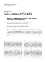
(18)
Figure 1 demonstrates the magnitude of these elements.
From the figure, it is obvious that, only when Q is large
enough and there is no frequency close to zero or 2π,can
F
T

Q
(F
T
Q
)
∗
/Q be approximated as an identity matrix and the
above method works. In practical applications, when this
condition is not satisfied, we need to consider alternative
approaches.
Jian (Andrew) Zhang et al. 5
0.2
0.4
0.6
0.8
1
Magnitude of correlation
6
4
2
0
Radian
0
2
4
6
Radian
(a) Correlation
0.2
0.4

0.6
0.8
1
Magnitude
70
60
50
40
30
Length Q
−5
0
5
Radian
(b) Element of matrix
Figure 1: Illustration of the entries of F
T
Q
(F
T
Q
)
∗
: (a) magnitude of correlation coefficients for a fixed Q = 50; (b) magnitude of the elements
in (18)versusvariousQ and the difference ω

1
−ω

2

.
The two key factors in the derivation of (17) are that (1)
Y
1
is symmetric and (2) a

,  ∈ [1, L] is fully contained in a
diagonal matrix, and each of them can be mapped to one of
the diagonal elements uniquely. These observations motivate
us to construct the following M
×Q data matrices
Y
1
=
⎛
⎜
⎜
⎜
⎜
⎝
x(0) x(−1) ··· x(1 −Q)
x(1) x(0)
··· x(2 −Q)
.
.
.
.
.
.
.

.
.
.
.
.
x(M
−1) x(M −2) ··· x(M − Q)
⎞
⎟
⎟
⎟
⎟
⎠
=
F
M
AF
∗
Q
,
Y
2
=
⎛
⎜
⎜
⎜
⎜
⎝
x(d) ··· x(d +1− Q)

x(d +1)
··· x(d +2− Q)
.
.
.
.
.
.
.
.
.
x(M
−1+d) ··· x(M − Q + d)
⎞
⎟
⎟
⎟
⎟
⎠
=
F
M
Φ
d
AF
∗
Q
,
(19)
where min

{M, Q}≥L and d ≥ 1.
These two matrices have the shift-invariant property,
and the diagonal elements of Φ can be determined by the
generalized eigenvalues of the matrix pencil (Y
1
− ξY
2
). The
reduced rank algorithms described in Proposition 2 are also
applicable to this pencil. Now, if we let M
= Q,andassume
A is a real matrix (a

are real), Y
1
will be a Hermitian
matrix. For a Hermitian but not necessarily positive-definite
matrix, the eigenvalues are real but not necessarily positive.
Therefore, to maintain its singular values positive, the left
and right singular vectors of the matrix are equal up to a
constant diagonal matrix

I. This matrix

I has diagonal entries
−1 or 1 corresponding to the polarity of the eigenvalues. For
example, U
p
= V
p


I
p
for the p principal singular vectors.
Then, similar to the proof of Proposition 3, the following
proposition can be proven. Note that the matrices P in
(A.1) in the proof of Proposition 3 will be replaced by A.
This change leads to the estimates of amplitudes rather than
squared amplitudes.
Proposition 4. When Y
1
and Y
2
are constructed in the way
similar to (19) with M
= Q,andA is a real diagonal matrix
w ith diagonal entries equal to the amplitudes of harmonic s, the
amplitude of th harmonic, a

,canbedeterminedby
a

=
θ
∗


I
p
Λ

p
θ



θ
∗


I
p
U
∗
p
f(M; ω

)


2
, (20)
where θ

is the generalized eigenvector corresponding to the
generalized eigenvalue ξ

(and then frequency ω

).
It is obvious that this result is superior to the one

in Proposition 3 in the estimation of a

. However, there
is another problem associated with it. Since Y
1
is a Her-
mitian matrix directly constructed from the samples, the
performance of the frequency estimation might be inferior
to the one in Proposition 3 when the dimensions of these
two matrices are equal. This happens when the added noise
matrix is also Hermitian, because in this case, the number
of effective samples in Proposition 4 equivalently reduces to
half. Even so, it might still be worthy of constructing a double
size matrix and using our RIPC algorithms when fast algo-
rithms can largely reduce the cost of computation, compared
to the general L-rank algorithms. This is confirmed by some
experimental results to be given in Section 5.
3.4. Fast algorithms to find the principal signal space
Since only p out of L principal singular values and vectors are
required, the computation can be simplified by applying fast
6 EURASIP Journal on Wireless Communications and Networking
0.5
0.6
0.7
0.8
0.9
1
Hit rate
0 5 10 15 20
Loops

(a) Hit rate of the frequency estimates
−60
−58
−56
−54
−52
−50
−48
−46
MSE (dB)
0 5 10 15 20
Loops
(b) MSE of the frequency estimates
0.58
0.6
0.62
0.64
0.66
0.68
0.7
Ratio of energy
0 5 10 15 20
Loops
(c) The ratio of collected energy
70
80
90
100
110
120

Iterations
0 5 10 15 20
Loops
(d) Iterations in the power method
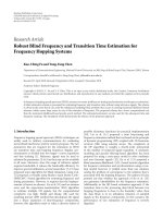
Figure 2: Implementations of A1–A5 in the noise-free case with p = 10, L = 50, and M = 60. Stems marked with diagonals, downward
triangles, circles, stars, and squares denote the algorithms A1–A5, respectively. These legends also apply to Figure 3.
algorithms with lower complexity, such as the power method
[19]. For each dominant singular value and vector, the power
method has a computational order of M
2
for an M × M
Hermitian matrix. To be stated, in the power method, the
speed of convergence depends on the ratio between the two
largest singular values of the matrix. The larger the ratio is,
the faster it converges.
For an M
× M Hermitian matrix Y
1
, the power method
generates p principal singular values and vectors as shown in
Algorithm 1.
When Y
1
is not a Hermitian matrix, a similar algorithm
is applicable in which the left and right singular vectors
should be generated by constructing Y
1
Y
∗
1

and Y
∗
1
Y
1
,
respectively.
On the detailed implementation of the power method,
we have some interesting findings in our experiments.
(i) After the ith eigenvector is generated, if we let it be
the initial iterative vector q
(0)
in solving the next
eigenvalue and vector rather than randomly chosen
q
(0)
, the iteration usually converges very fast. For
positive Hermitian matrices, 2 or 3 iterations are
enough.
(ii) Even when the first several estimated eigenvalues
contain larger errors, the remaining eigenvalues can
still be estimated with higher accuracy due to the
stability of eigenvalues to the perturbation errors.
(iii) If not all eigenvalues are positive, the power method
might output eigenvalues in a nonordered manner.
This usually implies relatively larger errors in these
eigenvalues. However, the estimated frequencies can
stillhavegoodaccuracy.
Jian (Andrew) Zhang et al. 7
0.5

0.6
0.7
0.8
0.9
Hit rate
0 5 10 15 20
Loops
(a) Hit rate of the frequency estimates
−58
−56
−54
−52
−50
−48
−46
MSE (dB)
0 5 10 15 20
Loops
(b) MSE of the frequency estimates
0.32
0.34
0.36
0.38
0.4
0.42
0.44
0.46
0.48
Ratio of energy
0 5 10 15 20

Loops
(c) The ratio of collected energy
44
46
48
50
52
54
Iterations
0 5 10 15 20
Loops
(d) Iterations in the power method
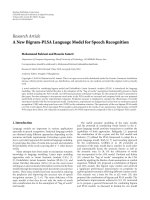
Figure 3: Implementations of A1–A5 with p = 5, L = 50, SNR = 5dB,andM = 60.
It should be noted that although the generalized eigenvalues
of the pencil (Y
1
−ξY
2
) are equal to the eigenvalues of (Y
†
2
Y
1
),
the power method is ineffective in directly solving the first
p eigenvalues of (Y
†
2
Y
1

) because there are not large enough
gaps between adjacent eigenvalues (the magnitudes of all
eigenvalues equal 1).
4. JOINT SYNCHRONIZATION AND
CHANNEL IDENTIFICATION
We consider a general transmitted UWB signal s(t)in
a single-user system. The signal s(t) could be a spread
spectrum (SS) signal (e.g., time-hopping or direct sequence
spread) or non-SS signal (e.g., single pulse), but it should be
unmodulated or modulated with known constant data. For
randomly modulated signals, the sampled channel impulse
response can be estimated using the least squares criterion
first as discussed in [4]. We assume that the spread spectrum
codes are known in an SS system.
Here, the used UWB multipath channel model is a
simplified version of the IEEE802.15.3a channel model [15],
which is a modified Saleh-Valenzuela model where multipath
components arrive in clusters. For synchronization and
channel estimation, the IEEE model can be simplified to a
TDL model, represented by
h(t)
=
L

=1
a

δ

t −τ



, (21)
where τ

is the th multipath delay, a

is the th multipath
gain with phase randomly set to
{±1}with equal probability,
L is the number of multipaths, and δ(
·) is the Dirac delta
8 EURASIP Journal on Wireless Communications and Networking
0.55
0.6
0.65
0.7
0.75
0.8
0.85
0.9
0.95
Mean hit rate
024681012141618
SNR (dB)
A1
A1
s
A2
A3

A4
A5
(a) Mean hit rate of the frequency estimates
10
−5
MSE
024681012141618
SNR (dB)
A1
A1
s
A2
A3
A4
A5
(b) Averaged MSE of the frequency estimates
Figure 4: The averaged hit rate (a) and MSE (b) versus the SNR in
the algorithms A1–A5 when p
= 10, L = 50, and M = 60 for A1,
A1
s
,A3,M = 120 for others.
function. The multipath delay τ

and gain a

are regarded as
deterministic parameters to be estimated.
When a symbol sequence
{s

i
(t)} is transmitted over this
channel, the received signal r(t)is
r(t)
=

i
L

=1
a

s
i

t −iT
s
−τ −τ


+ n(t), (22)
where n(t) is the additive white Gaussian noise (AWGN),
τ is the synchronization delay between the receiver and the
transmitter, and T
s
is the symbol period.
To set up the connection between (22)and(1), we can
transform (22) from time domain to frequency domain by
(1) Let i = 1, and set the desired number of
iterations to J in the calculation of every

singular value and vector(Note: Besides
this pre-defined J, a threshold can also be
set to jump out the iterations once the
squared error between two latest generated
eigenvalues is smaller than this threshold.);
(2) Generate the dominant real eigenvalue λ
i
=
λ
(J)
i
and left eigenvector u
i
= u
(J)
i
of Y
1
using the power method described below:
Generate a unit 2-norm vector q
(0)
∈ C
M
randomly;
for j
= 1, 2, , J
u
(j)
i
= Y

1
q
(j−1)
q
(j)
= u
(j)
i
/


u
(j)
i


2
λ
(j)
i
=

q
(j)

∗
Y
1
q
(j)

end
where
·
2
is the vector 2-norm;
(3) If λ
i
< 0, let λ
i
=−λ
i
, and the right
eigenvector v
i
be v
i
=−u
i
;Otherwise,let
v
i
= u
i
;
(4) Use the deflation operation to update Y
1
:
Y
1
= Y

1
−λ
i
u
i
v
∗
i
;
(5) Let i
= i + 1, and repeat 2 until i = p +1.
Algorithm 1: Algorithm to generate p principal singular values
and vectors of a M
× M Hermitian matrix Y
1
using the power
method.
applying the Discrete Fourier Transform (DFT) upon the
samples of r(t).
4.1. Sampling of signals
Since the system is not synchronized yet, whatever the signal
s(t) is, the width of the sampling window should be chosen
to equal the integral multiple of the symbol period and be
larger than the maximal multipath spread T
m
. Assume that
the sampling period is T, the number of samples is K
1
,and
the samples from (22)are

{r(m)}, m ∈ [0, K
1
− 1]. Two
scenarios regarding to the sampling need to be considered.
(1) Sampling of widely separated pulses
When the intervals between the continuously transmitted
pulses are larger than T
m
, there is no ISI in the samples.
Let the sampling length TK
1
equal the symbol period T
s
,
{s(m)} be the samples of s
i
(t), and {n(m)} be the samples
of the noise n(t), then the DFT coefficients of (22)canbe
represented as
R(k)
= S(k)
L

=1
a

e
−jkΩ
0
(τ+τ


)
+ N(k), k ∈

0, K
1
−1

,
(23)
where Ω
0
= 2π/(TK
1
) is the basic frequency, S(k)andN(k)
are the DFT coefficients of
{s(m)} and {n(m)},respectively.
Jian (Andrew) Zhang et al. 9
0.5
0.55
0.6
0.65
0.7
0.75
0.8
0.85
0.9
Mean hit rate
024681012141618
SNR (dB)

A1
A1
s
A2
A3
A4
A5
(a) Mean hit rate of the delay estimates
10
−5
MSE
02 4681012141618
SNR (dB)
A1
A1
s
A2
A3
A4
A5
(b) MSE of the delay estimates
Figure 5: The averaged hit rate (a) and MSE (b) versus the SNR in
the algorithms A1–A5 when p
= 10, L = 50, and M = 60 for A1,
A1
s
,A3,M = 120 for others. The parameters of harmonics are from
the IEEE channel model.
(2) Sampling of closely spaced pulses
When the intervals between the transmitted pulses are

smaller than T
m
, ISI is generated. Assume that the multipath
can be fully covered by at most Δi symbols, that is, T
s
Δi ≥
T
m
. Represent the Δi symbols as
s
Δi
(t) =
i
1
+Δi−1

i=i
1
s
i

t −iT
s

, (24)
where i
1
is the index of any symbol, and let {s(m)}, m ∈
[1, K
1

] be the samples of s
Δi
(t). In this case, the samples
0.3
0.35
0.4
0.45
0.5
0.55
0.6
0.65
0.7
Ratio of collected energy
024681012141618
SNR (dB)
A1
A2
A3
A4
A5
Mean energy of 10 largest taps
Figure 6: The mean ratio of the collected energy by A1–A5,
corresponding to the results in Figure 5.
of r(t), {r(m)}, contain ISI terms. However, when symbols
are transmitted continuously without interruption, it can be
proven that R(k), the DFT coefficients of
{r(m)}, are ISI-free
due to the Circular Shift Property [20, page 536] of DFT, and
(23) also holds.
This finding enables continuous transmission of the

training sequence to speed the synchronization process. This
is also another advantage of the proposed algorithms com-
pared to conventional algorithms which generally require
the interval between two impulses to be larger than the
multipath delay spread.
4.2. Summary of joint synchronization and channel
identification schemes using RIPC algorithms
Deconvolution is defined as the operation of dividing R(k)
by S(k)in(23), the reverse of convolution viewed in
the frequency domain. After the deconvolution operation,
we get some equations identical to (1) in the harmonic
retrieval problem. Then the synchronization and channel
identification algorithm can be summarized as follows:
(1) in a window with width TK
1
, sample the received
signal with period T.MakesureTK
1
equals an
integral multiple of the symbol period T
s
and larger
than the multipath spread T
m
;
(2) apply the FFT to the samples and select K DFT
coefficients carefully;
(3) after deconvolution, form the Hankel data matrix X,
and use principal components tracking algorithms
to estimate the p delays with largest energy (sum

of τ and τ

). (If the amplitudes a

are required,
correlation matrices or Hermitian data matrices
should be used.)
(4) resolve τ and τ

from the estimated delays.
10 EURASIP Journal on Wireless Communications and Networking
0.04
0.06
0.08
0.1
0.12
0.14
0.16
0.18
0.2
RMSE of delay
2 4 6 8 10 12 14 16 18 20 22 24
CIR
A5 mean 0.12
A4 mean 0.09
A2 mean 0.07
(a)
0
0.1
0.2

0.3
0.4
Mean error of gain
2 4 6 8 10 12 14 16 18 20 22 24
The means over realizations are: 0.13 (A2), 0.09 (A4) and 0.16 (A5).
(b)
0.3
0.4
0.5
0.6
0.7
0.8
0.9
1
Hitting rate of delay
2 4 6 8 10 12 14 16 18 20 22 24
The means over realizations are: 0.8 (A2), 0.83 (A4) and 0.7 (A5).
A2
A4
A5
(c)
Figure 7: Performance of estimates in the noise-free case when T =
0.3t
p
, p = 10, L = 50, and M = 60. From top to bottom: normalized
RMSEs of the delay estimates, mean errors of the gain estimates and
hit rates of the delay estimates. The horizontal axis in each subplot
represents CIR realizations.
The last step is necessary as each estimated delay in step
(3) is the sum of the synchronization delay τ and one of

the multipath delays τ

. There is a phase-ambiguity problem
with these sums as the delays may become circularly shifted.
This could happen when sampling starts in the middle of
multipath delays. Our solution is first to choose TK
1
much
larger than the maximal multipath delay T
m
, then separate τ
and τ

according to the following criteria.
0.1
0.11
0.12
0.13
0.14
0.15
0.16
0.17
0.18
Normalized RMSE
012345 678910
SNR (dB)
A2
A4
A5
Root

squared
CRLB
Figure 8: Normalized RMSE of the delay estimates versus the SNR
where T
= 0.3t
p
, p = 10, L = 50, and M = 60.
(i) Sort the estimates in ascending order and get
{τ
1
, τ
2
, , τ
p
}. If the gap between any two adjoining
estimates is larger than a threshold τ
th
,forexample,
τ
p
1
− τ
p
1
−1
>τ
th
, then τ
p
1

equals the sum of
the synchronization delay τ and the first desired
multipath delay. And all the estimates need to be
updated to

τ
p
1
, τ
p
1
+1
, , τ
p
, τ
1
+ TK
1
, , τ
p
1
−1
+ TK
1

,
(25)
that is, the original
τ
1

, , τ
p
1
−1
are updated by
adding TK
1
to themselves. Now, the receiver can
synchronize to the multipath with delay
τ
p
1
which
implicitly assumes the delay of the first multipath
of interest is zero, and the differences between the
updated estimates and the first desired multipath are
the relative multipath delays.
(ii) Otherwise, the smallest estimate is the first multipath
of interest and no update is needed.
This judgement is based on the assumption that the gap
between any two multipath signals is smaller than the thresh-
old τ
th
, which is generally close to the difference between
the sampling window width TK
1
and the maximal multipath
delay T
m
. In practice, the multipath components with larger

energy usually have smaller delays, so the threshold τ
th
needs
not be very large.
4.3. Complexity of our schemes
The complexity of our algorithms depends on the required
resolution ability and performance of estimation. The
resolution ability is roughly determined by the sampling
Jian (Andrew) Zhang et al. 11
period. The smaller the sampling period is, the higher the
resolution ability is. The performance of estimation is mainly
influenced by the SNR, and the dimension of the matrices
Y
1
and Y
2
. Then the sampling period is the key parameter
in both the complexity and performance since the main
computation cost of our algorithm is associated with FFT,
SVD, and GED. For a K
1
-point FFT, the computational
workload is K
1
(3log
2
K
1
− 1)/2 when a Cooley-Tukey radix-
2 algorithm [21]isused.K

1
equals a power of 2. The
complexity of GED for a p
× p matrix is p
3
. Plus the
complexity of the power method (suppose that K
= K
1
/2
DFT coefficients are used), the total complexity is in the
order of K
1
log
2
K
1
+ pK
2
1
/4+p
3
. Accordingly, the complexity
of the general L-rank algorithms is in the order of K
1
log
2
K
1
+

K
3
1
/8+L
3
. When L  p, the saving is considerable.
5. SIMULATIONS
First, we show some experimental results of the RIPC algo-
rithms using the harmonic retrieval model. The performance
can act as a basis for evaluating the performance loss in many
applications of RIPC algorithms. Simulation results of the
joint synchronization and channel identification for UWB
signals are given in Section 5.2.
5.1. Simulations of RIPC algorithms
The simulations in this subsection are based on the harmonic
retrieval model in (1). The algorithms evaluated are classified
as follows.
(A1) Algorithms A1 are full L-rank algorithms with a
general matrix Y
1
(not Hermitian nor positive-
definite), where amplitudes are obtained by solving
a Vandermonde problem using the least squares
criterion.
(A2) Algorithms A2 are full L-rank algorithms with a
Hermitian matrix Y
1
(not positive-definite), where
amplitudes can be estimated via (20) or by solving
a Vandermonde matrix.

(A3) Algorithms A3 are RIPC algorithms with a general
matrix Y
1
, where amplitudes cannot be estimated.
(A4) Algorithms A4 are RIPC algorithms with a Hermitian
matrix Y
1
, where amplitudes are estimated by (20).
(A5) Algorithms A5 are RIPC algorithms with a Hermitian
matrix Y
1
, where the power method is applied and
amplitudes are estimated by (20).
We first generate amplitudes a

randomly using a
Gaussian distribution with mean zero and variance 1. These
amplitudes are normalized such that their squared sum
is unity. The frequencies are generated randomly using a
uniform distribution on the interval [0, 2π). In most cases,
L
= 50 harmonics are generated, and 60 × 60 matrices Y
1
and Y
2
are constructed.
Figures 2 and 3 demonstrate some detailed implemen-
tations of algorithms A1–A5. Each figure consists of 4
subfigures. Figures 2(a) and 3(a) shows the hit rate of the
frequency estimates. When an estimate has an estimation

error within a predefined threshold (named as “hitting
threshold” hereafter, set to 0.01), we say it “hits” the true
value. The hit rate is then defined as the ratio between
the number of the hit estimates and the total estimates.
The hit rate is thus conceptually similar to the outage
probability that is commonly used in the literature. Figures
2(b) and 3(b) shows the mean squared error (MSE) of the
hit estimates (nonhit estimates are excluded) averaged over
10 realizations. The results obtained by algorithms A1–A5
are denoted by diagonals, triangles (down), circles, stars,
and squares, respectively. Figures 2(c) and 3(c) shows the
energy ratio of the p principal harmonics out of the total
ones. Figures 2(d) and 3(d) shows the averaged number of
iterations in the power method. In the power method, the
maximal number of iterations in computing every eigenvalue
and vector (J in Algorithm 1 ) is set to 30, and the threshold
is set to 0.004 to control the number of iterations.
In Figure 2, simulation results in the noise-free case
are illustrated with p
= 10 and L = 50. It is clear
that full L-rank algorithms A1 and A2 can achieve perfect
estimation with high hit accuracy and near zero MSEs (not
plotted in Figure 2(b)). Comparatively, our reduced-rank
RIPC algorithms can not achieve perfect estimation in the
noise-free case, while they are relatively stable with respect to
the change of SNR.
Even when the samples are corrupted by noise, the
algorithms A1 and A2 can normally achieve good frequency
estimates for some harmonics, as can be observed in Figures
2 and 3. However, their amplitude estimates usually contain

relatively larger error due to the following two reasons. On
the one hand, the frequency estimates with higher accuracy
normally correspond to the harmonics with larger energy
according to the Cramer-Rao bound. For frequencies with
smaller energy, the estimates inevitably contain larger errors.
On the other hand, the accuracy of frequency estimates is
due to the inherent stability of eigenvalues and singular
values. The amplitude estimates, however, are susceptible
to the noise. Thus, in the sense of determining p principal
frequencies with largest energy, A1 is less effective than RIPC
algorithms.
The ratio of collected energy shown in Figures 2 and
3(b) indicates that the hit rate and MSE are actually weakly
dependent of the collected harmonics energy. This implies
that an analytical analysis using an approximation theory
(or the perturbation theory) for Proposition 2 might not
work. Simultaneously, it implies that the stability of the RIPC
algorithmsishighwithrespecttothenumberp of the desired
principal signals.
Figure 4 demonstrates how the hit rate and MSE vary
with SNR where A1
s
is a state space based algorithm within
the framework of A1 used in [3]. From the figure, we see that
when the SNR is larger (than 5 dB), the performance of the
RIPC algorithms are satisfactory and stable.
In experiments, we find that the amplitude estimates in
the RIPC algorithms are not so accurate as the frequency
estimates because the errors in the frequency estimates are
actually transferred into the amplitude estimates. In most

cases, the polarity of the amplitude can be determined
12 EURASIP Journal on Wireless Communications and Networking
accurately, while the magnitude can suffer an error as
large as 30% of the true value in the SNR range 5–15 dB.
This is a general problem in the subspace-based harmonic
retrieval algorithms, which could be mitigated by averaging
over multiple realizations. However, this problem does not
influence the determination of p principal harmonics in
RIPC algorithms as they have been automatically tracked and
picked out during the frequency estimation.
5.2. Simulations of joint synchronization and
channel identification
The second-order Gaussian monocycle p(t) is used as the
basic pulse
p(t)
=
⎡
⎣
1 −4π

t −t
p
t
p

2
⎤
⎦
e
−2π((t−t

p
)/t
p
)
2
, (26)
where t
p
parameterizes the effective pulse width. The
−3 dB bandwidth of this pulse is about 0.65/t
p
Hz, −10 dB
bandwidth is about 1.15/t
p
Hz, and center frequency is about
0.8/t
p
Hz.
When sampling this pulse with period T
= 0.3t
p
,we
get roughly six samples per pulse, and this sampling rate
is already above the Nyquist rate in terms of the
−10 dB
bandwidth. To reduce the sampling rate without introducing
aliasing, similar to [3], a low-pass filter with bandwidth
much smaller than the signal bandwidth can be applied at
the cost of reduced energy collection. When choosing “clean”
DFT coefficients to minimize interference due to residual

alias, coefficients near the normalized frequency 0.5 should
be excluded. On the other hand, DFT coefficients with larger
energy should be chosen to avoid blowing up the noise
in the deconvolution operation. When strong narrowband
interference is present and the interference spectrum is
known, the interference can be readily removed by selecting
those coefficients in the unaffected spectrum.
To test the performance of our algorithms in practical
implementations, we use the channel model CM1 proposed
in [15] by IEEE802.15.3a. The channel impulse response
(CIR) is reproduced using t
p
= 10
−9
. The first L = 50
multipath signals in each CIR are used to simulate the
channel.
Before the actual implementations of synchronization
and channel estimation, we first feed these multipath param-
eters into the harmonic retrieval model, that is, substitute
a

with the multipath gains and ω

with 2πτ

/TK
1
in (1),
where TK

1
is chosen to be slightly larger than the maximal
multipath delay T
m
. The achievable performance can serve
as upper bounds in practical implementations.
Figure 5 shows the hit rate and MSE of the frequency
estimates in this case, and the actual collected energy by
these algorithms is shown in Figure 6. To make the estimates
independent of TK
1
, estimates are kept in the form of
frequencies rather than delays. It can be seen that there is
notmuchdifference between the performance here and that
shown in Figure 4. This indicates the stability of our RIPC
algorithms. From Figure 6, we can also see that about 80%
energy of the 10 largest channel taps can be collected (and
exploited then), which is consistent with the hit rate.
To check the performance loss in practical implementa-
tions, let us examine the noise-free case first. In the noise-free
experiments, DFT coefficients from 0 to 0.4K
1
are chosen,
the hitting threshold is set to 0.25t
p
, and the estimates are
compared with 15 principal multipath signals to determine
the hits. Figure 7 shows the hit rate, root MSE (RMSE) of
the delay estimates and mean error of the gain estimates
obtained by A2, A4, and A5 with p

= 10, L = 50, and
M
= 60. The RMSEs of the delay estimates are normalized
with respect to t
p
. The sampling rate is 0.3t
p
.InFigure 8,
we show the RMSEs of the delay estimates versus the SNR
for A2, A4, and A5. For comparison, the Cramer-Rao low
bound (CRLB) in an AWGN channel [16] is also plotted.
From the figures, we can see that an accuracy of about
10% of T
p
canbeobtainedataveragehitrateabove80%.
This means that the timing accuracy is mostly within one
sample distance, which is only slightly inferior to the full-
rank approach in [3]. When the SNR is as large as 10 dB,
the RMSEs are already very close to those in the noise-free
case. Overlapping of the CRLB curve with other performance
curves is due to the lower hit rate at smaller SNRs, where
quite a few estimates with larger errors are excluded from
the computation of the MSE. With the hit rate increasing,
the CRLB curve becomes a good reference for evaluating the
performance of the proposed schemes.
6. CONCLUSIONS
To reduce the complexity of general subspace-based delay
estimation algorithms, we proposed reduced-rank shift-
invariant techniques which can track the principal com-
ponents automatically. Amplitude estimation schemes are

also proposed based on subspace methods. Application of
the proposed techniques in synchronization and channel
estimation for UWB signals is investigated. Experiments
show that our proposed algorithms can achieve performance
comparable to full-rank algorithms, but with significantly
reduced complexity.
APPENDIX
Proof of Proposition 3. Substitute (3) into (16), we get
Y
1
= F
(M−d)
AF
T
Q

F
T
Q

∗
A
∗

F
(M−d)

∗
≈ QFPF
∗

,
Y
2
= F
(M−d)
Φ
d
AF
T
Q

F
T
Q

∗
A
∗

F
(M−d)

∗
≈ QFΦ
d
PF
∗
,
(A.1)
where A is the diagonal matrix defined in (4), F

T
Q
(F
T
Q
)
∗
approximates an identity matrix up to a multiplicative
scalar Q since over intervals of infinite support, cisoids of
different frequencies are orthogonal [8]. Thus, the product
AF
T
Q
(F
T
Q
)
∗
A
∗
/Q can be replaced by a diagonal matrix P with
diagonal entries equal to the energy of harmonics, that is, P
=
diag (|a
1
|
2
, |a
2
|

2
, , |a
L
|
2
). Temporarily, we denote F
(M−d)
by F for brevity.
Jian (Andrew) Zhang et al. 13
Since Y
1
is a Hermitian matrix and positive-definite,
its left and right singular vectors are identical. Let θ

be
the generalized eigenvector corresponding to the generalized
eigenvalue ξ

. According to the definition of the generalized
eigen-problem, for the pencil Λ
p
−ξU
∗
p
Y
2
V
p
,wehave
U

∗
p
FP

I −ξ

Φ
d

F
∗
U
p
θ

= 0,(A.2)
where the expressions of Y
1
and Y
2
in (A.1)areused.Left
multiplied by θ
∗

,(A.2)becomes

θ
∗

U

∗
p
F

P

I −ξ

Φ
d

θ
∗

U
∗
p
F

∗
= 0. (A.3)
Since P(I
− ξ

Φ
d
)isanL × L diagonal matrix with only the
th diagonal element equal to zero, the 1
× L vector θ
∗


U
∗
p
F
has the form
θ
∗

U
∗
p
F =

0, ,0,θ
∗

U
∗
p
f(M − d; ω

), 0, ,0

,(A.4)
that is, except for the th element, all others equal zero.
Notice that Λ
p
= U
∗

p
Y
1
U
p
and ξ

Φ
d
is a diagonal matrix
with the th diagonal element equal to one. Hence, (A.3)can
be rewritten as
θ
∗

Λ
p
θ

=

θ
∗

U
∗
p
F

Pξ


Φ
d

θ
∗

U
∗
p
F

∗
=


a



2


θ
∗

U
∗
p
f


M − d; ω




2
,
(A.5)
which establishes (17).
ACKNOWLEDGMENTS
NICTA is funded by the Australian Government as repre-
sented by the Department of Broadband, Communications
and the Digital Economy and the Australian Research
Council through the ICT Centre of Excellence program.
REFERENCES
[1] E. A. Homier and R. A. Scholtz, “Rapid acquisition of
ultra-wideband signals in the dense multipath channel,” in
Proceedings of the IEEE Conference on Ultra Wideband Systems
and Technolog ies (UWBST ’02), pp. 105–109, Baltimore, Md,
USA, May 2002.
[2] V. Lottici, A. D’Andrea, and U. Mengali, “Channel estimation
for ultra-wideband communications,” IEEE Journal on Selected
Areas in Communications, vol. 20, no. 9, pp. 1638–1645, 2002.
[3] I. Maravi
´
c, J. Kusuma, and M. Vetterli, “Low-sampling rate
UWB channel characterization and synchronization,” Journal
of Communications and Networks, vol. 5, no. 4, pp. 319–326,
2003.

[4] A J. van der Veen, M. C. Vanderveen, and A. Paulraj, “Joint
angle and delay estimation using shift-invariance techniques,”
IEEE Transactions on Signal Processing, vol. 46, no. 2, pp. 405–
418, 1998.
[5] A. L. Swindlehurst, “Time delay and spatial signature estima-
tion using known asynchronous signals,” IEEE Transactions on
Signal Processing, vol. 46, no. 2, pp. 449–462, 1998.
[6] B. D. Rao and K. S. Arun, “Model based processing of signals:
a state space approach,” Proceedings of the IEEE, vol. 80, no. 2,
pp. 283–309, 1992.
[7]A J.vanderVeen,E.F.Deprettere,andA.L.Swindlehurst,
“Subspace-based signal analysis using singular value decom-
position,” Proceedings of the IEEE, vol. 81, no. 9, pp. 1277–
1308, 1993.
[8] R. Roy, A. Paulraj, and T. Kailath, “ESPRIT—a subspace
rotation approach to estimation of parameters of cisoids in
noise,” IEEE Transactions on Acoustics, Speech, and Signal
Processing, vol. 34, no. 5, pp. 1340–1342, 1986.
[9] R. Roy and T. Kailath, “ESPRIT-estimation of signal param-
eters via rotational invariance techniques,” IEEE Transactions
on Acoustics, Speech, and Signal Processing,vol.37,no.7,pp.
984–995, 1989.
[10] Y. Hua and T. K. Sarkar, “On SVD for estimating generalized
eigenvalues of singular matrix pencil in noise,” IEEE Transac-
tions on Signal Processing, vol. 39, no. 4, pp. 892–900, 1991.
[11] L. L. Scharf and D. W. Tufts, “Rank reduction for modeling
stationary signals,” IEEE Transactions on Acoustics, Speech, and
Signal Processing, vol. 35, no. 3, pp. 350–355, 1987.
[12] L. L. Scharf, “The SVD and reduced rank signal processing,”
Signal Processing, vol. 25, no. 2, pp. 113–133, 1991.

[13] L. L. Scharf, Statistical Signal Processing: Detection, Estimation,
and Time Series Analysis, Addison-Wesley, New York, NY,
USA, 1991.
[14] Y. Hua, M. Nikpour, and P. Stoica, “Optimal reduced-
rank estimation and filtering,” IEEE Transactions on Signal
Processing, vol. 49, no. 3, pp. 457–469, 2001.
[15] J. Foerster, “Channel modeling sub-committee report final,”
IEEE P802.15 Working Group for Wireless Personal Area
Networks (WPANs), IEEE P802.15-02/490r1-SG3a,February
2003.
[16] J. Zhang, R. A. Kennedy, and T. D. Abhayapala, “Cram
´
er-
Rao lower bounds for the synchronization of UWB signals,”
EURASIP Journal on Applied Signal Processing, vol. 2005, no.
3, pp. 426–438, 2005.
[17] X D. Zhang and Y C. Liang, “Prefiltering-based ESPRIT
for estimating sinusoidal parameters in non-Gaussian ARMA
noise,” IEEE Transactions on Signal Processing, vol. 43, no. 1,
pp. 349–353, 1995.
[18] F. Zhang, Matrix Theory: B asic Results and Techniques,
Springer, New York, NY, USA, 1999.
[19] G. H. Golub and C. F. V. Loan, Matrix Computations,The
Johns Hopkins University Press, Baltimore, Md, USA, 3rd
edition, 1996.
[20] A. V. Oppenheim and R. W. Schafer, Discrete-Time Signal
Processing, Prentic-Hall, London, UK, 1989.
[21] D. F. Elliott, Ed., Handbook of Digital Signal Processing:
Engineering Applications, Academic Press, San Diego, Calif,
USA, 1987.